Unrelated Parallel Machine
Scheduling Problem:
A Cement Industry Case Study
Departamento de Produção e Sistemas
João Manuel Silva Fonseca
Unrelated Parallel Machine
Scheduling Problem:
A Cement Industry Case Study
Mestrado em Engenharia de Sistemas
Trabalho realizado sob orientação de
Professor Doutor José António Vasconcelos Oliveira
Professor Doutor Luís Miguel Silva Dias
DECLARAC
¸ ˜
AO
Nome: Jo˜ao Manuel Silva Fonseca Endere¸co eletr´onico: [email protected]
T´ıtulo da Disserta¸c˜ao: Unrelated Parallel Machine Scheduling: A Cement Industry Case Study
Orientadores:
Professor Doutor Jos´e Ant´onio Vasconcelos Oliveira Professor Doutor Lu´ıs Miguel Silva Dias
Ano de conclus˜ao: 2018
Mestrado em Engenharia de Sistemas
´
E AUTORIZADA A REPRODUC¸ ˜AO INTEGRAL DESTA DISSERTAC¸ ˜AO
APENAS PARA EFEITOS DE INVESTIGAC¸ ˜AO, MEDIANTE DECLARAC¸ ˜AO
ESCRITA DO INTERESSADO, QUE A TAL SE COMPROMETE.
Universidade do Minho, - -O Autor:
To my parents. . .
Acknowledgements
This document ends an important stage of my life. I use this space to express my gratitude to those who have helped me in so many ways.
To my supervisors, Jos´e Ant´onio Oliveira, Ph.D. and Lu´ıs Dias, Ph.D., for the total availability, opinions, criticisms and for opening up the scientific research world to me. To my family. Without them, this journey would not be possible. To my parents, to whom I dedicate this dissertation, for my education and for giving me great values, which I take to life. To my brother, for the constant support and to Filomena Alves, who always treated me like a son.
To Francisca Fonseca, who makes me a better man, every day. For being my confidant, for her love and affection, for her good mood, patience and for always being by my side. To Ricardo Alves and Regina Macedo, who walked on this journey with me. For being the best group of work, for all the advice and words of encouragement, but specially for their friendship.
To Andr´e Souto, Afonso Rodrigues, Joaquim Santos, Miguel Nogueira, Miguel Sanches, Rui Costa and Z´e Bruno, who accompanied me in these five years of learning. For the laughs, for their friendship and for being always prompt to help.
UNIVERSITY OF MINHO
Abstract
School of Engineering
Department of Production and Systems
by Jo˜ao Manuel Silva Fonseca
This dissertation considers the problem of scheduling unrelated parallel machines, with unequal release dates and machine eligibility constraints, to minimize the total flow time of the system. It establishes an analogy between this problem and an existing process in the cement industry – the loading of trucks by the customers. Hence, it intends to find opportunities for improvement in the reduction of the customers’ interaction times and in their experience inside the cement plants. To achieve this goal, three optimiza-tion models are proposed, one exact and two heuristics. Also, an extensive series of computational tests are carried out to compare the performance of the methods. The exact method, based on a mathematical formulation of the problem, requires a high computational time and it is incapable of dealing with large instances. Consequently, it is not a viable solution for an industrial sized problem. However, it contributes to a better understanding of the structure of the problem and to develop efficient heuristics. The heuristics, one based on dispatching rules and the other on a simulated annealing algorithm, show potential for the implementation in a real life scenario. Although simu-lated annealing gives considerably better solutions than the other heuristic, it takes more time to give results and it is more complex to implement. The dispatching rules based heuristic gives solutions almost instantly and more easily includes certain characteris-tics of the problem. In general, these methods improve the quality of service provided, reducing the overall time the customers are spending inside the cement plants. Thus, cement industry can and should use optimization models to improve their operations and the customers’ experience.
Keywords: Cement Industry, Machine Scheduling, Optimization Models, Mathematical Pro-gramming, Dispatching Rules, Simulated Annealing, Total Flow Time.
Supervised by:
Ph.D. Professor Jos´e Ant´onio Oliveira Ph.D. Professor Lu´ıs Dias
UNIVERSIDADE DO MINHO
Resumo
Escola de Engenharia
Departamento de Produ¸c˜ao e Sistemas
feito por Jo˜ao Manuel Silva Fonseca
Esta disserta¸c˜ao considera o problema de agendamento de m´aquinas paralelas n˜ao rela-cionadas, com datas de disponibilidades diferentes e restri¸c˜oes de elegibilidade, para minimizar o tempo total de fluxo do sistema. Esta estabelece tamb´em uma analogia entre este problema e um processo existente na ind´ustria cimenteira – o carregamento de cami˜oes pelos clientes. Assim, pretende encontrar oportunidades de melhoria na redu¸c˜ao dos tempos de intera¸c˜ao dos clientes e na sua experiˆencia dentro das cimenteiras. Para atingir este objetivo, trˆes modelos de otimiza¸c˜ao s˜ao propostos, um exato e duas heur´ısticas. Al´em disso, uma extensa s´erie de testes computacionais ´e realizada para comparar o desempenho dos m´etodos. O m´etodo exato, baseado numa formula¸c˜ao matem´atica do problema, requer bastante tempo computacional e ´e incapaz de lidar com instˆancias grandes. Consequentemente, n˜ao ´e uma solu¸c˜ao vi´avel para um problema de tamanho industrial. No entanto, contribui para uma melhor compreens˜ao da estrutura do problema e para desenvolver heur´ısticas eficientes. As heur´ısticas, uma baseada em regras de despacho e a outra num algoritmo de simulated annealing, mostram poten-cial para uma implementa¸c˜ao num cen´ario da vida real. Embora o simulated annealing ofere¸ca solu¸c˜oes consideravelmente melhores do que a outra heur´ıstica, este necessita de mais tempo para fornecer resultados e ´e mais complexo de implementar. A heur´ıstica baseada em regras de despacho fornece solu¸c˜oes quase instantaneamente e pode incluir mais facilmente certas caracter´ısticas do problema. Em geral, estes m´etodos melhoram a qualidade do servi¸co prestado, reduzindo o tempo total que os clientes gastam dentro das cimenteiras. Assim, a ind´ustria cimenteira pode e deve usar modelos de otimiza¸c˜ao, para melhorar as suas opera¸c˜oes e a experiˆencia dos clientes.
Palavras-Chave: Ind´ustria Cimenteira, Agendamento de M´aquinas, Modelos de Otimiza¸c˜ao, Programa¸c˜ao Matem´atica, Regras de Despacho, Simulated Annealing, Tempo Total de Fluxo.
Orientado por:
Professor Dr. Jos´e Ant´onio Oliveira Professor Dr. Lu´ıs Dias
Contents
1 Introduction 1
Part I
State of the Art
2 Supply Chain Management 9
2.1 Definition and Overview . . . 9
2.2 Logistics Management . . . 11
2.3 Customer Service and Value . . . 13
3 Machine Scheduling 15 3.1 Background . . . 15 3.2 Problem Representation . . . 16 3.3 Complexity . . . 19 4 Solving Techniques 23 4.1 Mathematical Programming . . . 23
4.2 Constructive and Improvement Heuristics . . . 26
4.2.1 Dispatching Rules . . . 27
4.2.2 Simulated Annealing . . . 30
Part II
Case Study
5 Cement Industry 37 5.1 Contextualization . . . 375.2 Problem Description and Assumptions . . . 41
5.3 Approaches . . . 43
5.3.1 Mathematical Programming . . . 45
5.3.2 Dispatching Rule . . . 47
5.3.3 Simulated Annealing . . . 47
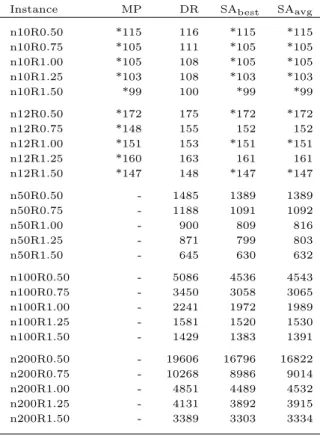
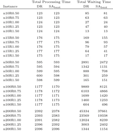
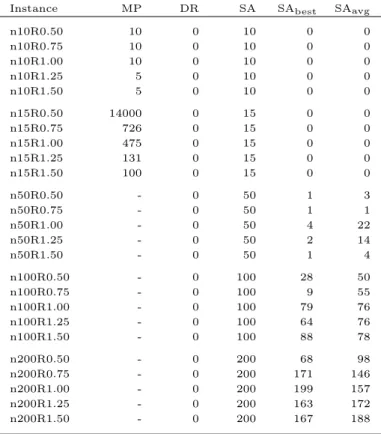
6 Tests and Results 53 6.1 Cement Plant I . . . 55
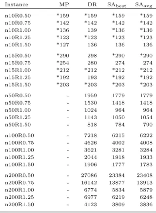
6.2 Cement Plant II . . . 57
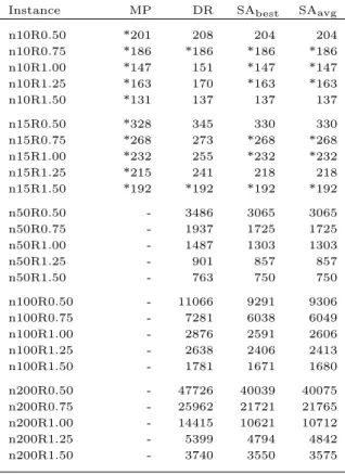
6.3 Cement Plant III . . . 59
7 Conclusions 67
A Cement Plant I 71
B Cement Plant II 81
C Cement Plant III 91
List of Figures
2.1 Basic SC and its main flows. . . 9
2.2 Logistics management process, as part of a SC. . . 11
2.3 Product and its added value through customer service. . . 13
3.1 Complexity hierarchy on the machine environment of scheduling problems. 20 3.2 Complexity hierarchy on jobs and machines characteristics. . . 21
3.3 Complexity hierarchy on the performance criteria considered. . . 21
4.1 Acceptance function behavior with T and ∆. . . 31
5.1 Important locations of a typical CP (SLV Cement by Cachapuz Bilanciai Group, n.d.). . . 38
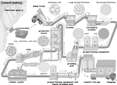
5.2 Cement manufacturing process, from raw material to end customer (Thomas and Lea, 2018). . . 40
5.3 Example of connections between silos and its respective LPs. . . 41
5.4 Example of a neighborhood solution by a switch. . . 50
5.5 Example of a neighborhood solution by a shift. . . 50
5.6 Example of a neighborhood solution by a swap. . . 51
5.7 Example of a neighborhood solution by a task move. . . 51
6.1 Combination between silos and LPs of CPI. . . 55
6.2 Combination between silos and LPs of CPII. . . 57
6.3 Combination between silos and LPs of CPIII. . . 59
6.4 SA improvements in CPIII. . . 61
6.5 Flow time behavior with R variation, using SA results. . . 63
6.6 Running time exponential behavior of the MP method. . . 65
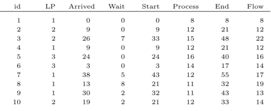
6.7 Example of Gantt chart, using the SA on the n10R1.00 instance. . . 66
A.1 SA improvements in CPI. . . 77
A.2 Flow time behavior with R variation, using the SA results. . . 78
A.3 Flow time behavior with R variation, using the DR results. . . 78
A.4 Running time exponential behavior of the MP method. . . 79
B.1 SA improvements in CPII. . . 87
B.2 Flow time behavior with R variation, using the SA results. . . 88
B.3 Flow time behavior with R variation, using the DR results. . . 88
B.4 Running time exponential behavior of the MP method. . . 89
C.1 Flow time behavior with R variation, using the DR results. . . 97
List of Tables
4.1 Analogy between the annealing process and a combinatorial optimization
problem. . . 32
6.1 Demand of each material available in CPI. . . 56
6.2 Flow time results in CPI. . . 56
6.3 Demand of each material available in CPII. . . 58
6.4 Flow time results in CPII. . . 58
6.5 Demand of each material available in CPIII. . . 59
6.6 Flow time results in CPIII. . . 60
6.7 Processing and Waiting Times Results in CPIII. . . 62
6.8 Running times of the computational tests in CPIII. . . 64
6.9 Example of schedule, using the SA on the n10R1.00 instance. . . 66
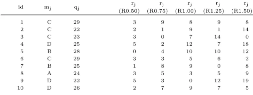
A.1 Generated data, for the customers of CPI - 10 jobs instance. . . 71
A.2 Generated data, for the customers of CPI - 12 jobs instance. . . 71
A.3 Generated data, for the customers of CPI - 50 jobs instance. . . 72
A.4 Generated data, for the customers of CPI - 100 jobs instance. . . 72
A.5 Generated data, for the customers of CPI - 200 jobs instance. . . 74
A.6 Processing and Waiting Times Results in CPI. . . 77
A.7 Running times of the computational tests in CPI. . . 79
B.1 Generated data, for the customers of CPII - 10 jobs instance. . . 81
B.2 Generated data, for the customers of CPII - 15 jobs instance. . . 81
B.3 Generated data, for the customers of CPII - 50 jobs instance. . . 82
B.4 Generated data, for the customers of CPII - 100 jobs instance. . . 82
B.5 Generated data, for the customers of CPII - 200 jobs instance. . . 84
B.6 Processing and Waiting Times Results in CPII. . . 87
B.7 Running times of the computational tests in CPII. . . 89
C.1 Generated data, for the customers of CPIII - 10 jobs instance. . . 91
C.2 Generated data, for the customers of CPIII - 15 jobs instance. . . 91
C.3 Generated data, for the customers of CPIII - 50 jobs instance. . . 92
C.4 Generated data, for the customers of CPIII - 100 jobs instance. . . 92
C.5 Generated data, for the customers of CPIII - 200 jobs instance. . . 94
Acronyms
ACO Ant Colony Optimization
CI Cement Industry
CP Cement Plant
DR Dispatching Rule
ECT Earliest Completion Time
EDD Earliest Due Date
ERD Earliest Release Date
FAM First Available Machine
FIFO First In First Out FCFS First Come First Served
GA Genetic Algorithm
HC Hill Climbing
ILS Iterated Local Search
LFJ Least Flexible Job
LP Loading Point
LPT Longest Processing Time
LST Least Slack Time
MS Machine Scheduling
MP Mathematical Programming
SA Simulated Annealing
SC Supply Chain
SCM Supply Chain Management
SPT Shortest Processing Time
SQ Shortest Queue
TS Tabu Search
UH4SP Unified Hub for Smart Plants xix
Chapter 1
Introduction
Contextualization
This dissertation emerges under the scope of the Unified Hub for Smart Plants (UH4SP) research project. In this project, the ALGORITMI Research Center, at University of Minho, joins several teams to help the company Cachapuz to take the current industry to another level. This company has its focus on the Cement Industry (CI), dealing with Cement Plants (CPs) geographically spread all over the world and with varied dimensions. Its main area of intervention is targeted to the control of logistics flows, seeking to improve all processes, from the entrance of a truck in the CP, to the cement delivery.
This research project appears at a time of renewal of this industry. The global market is changing from product oriented to customer oriented, and the CI also wants to make that change. Wanting to steer their businesses towards the customers, differentiated solutions that add value and promote a better level of service are sought. In order to develop the CI Supply Chain (SC), the UH4SP intends to introduce the concept of efficiency, effectiveness and intelligence to the CI. Here, the Smart Plant concept seeks to automate processes, reduce interaction times and improve the customers’ experience for the partners involved in the logistics processes.
The delivery of orders to customers is one of the areas that has great opportunities for improvement in this industry. The daily arrival of hundreds of customers to a CP, looking for their trucks to be loaded, is responsible for most of the entropy within the facilities. Long waiting and processing times, the disruption of operations, and others, are just examples of the consequences of incorrect handling of a high flow of customers. These lead to customer’s discontent and damages the service level, at the same time leading to high operating costs and inefficient use of resources and installed capacity.
In order to overcome this situation, the idea of scheduling, for the loading processes, aims to increase the organization within the CPs and to promote an improvement of the service levels. The scheduling of deliveries is one of the most important tasks in the Supply Chain Management (SCM), since it is directly linked to the customer. This is a process that determines the flow of resources and can be an indicator of the SC performance, through customer’s satisfaction. Ensuring the right product, at the right time, in the exact quantity, to the authorized person and in perfect conditions are challenges that require a high level of organization. In this context, optimization models, applied to logistics flows, assume a special importance in order to create a favorable agenda for both the company and its customers.
In this work, a scientific research will be carried out and it aims to address the problem described above. The themes of SCM and logistics processes, which are aimed at cus-tomer’s satisfaction, will be highlighted. An innovative approach to the loading schedule will be presented, establishing an analogy between the delivery of orders and the Ma-chine Scheduling (MS) problems. Three optimization models will be developed from scratch and presented as solutions to the problem in question. Their performances will be analyzed and conclusions will be drawn, aiming a future implementation in real life. The ambition is to create a new paradigm in the scheduling of loading trucks by the customers in the CI.
Objectives
Purposing to tackle the problems stated before, this dissertation intends to:
− Recognize the lack of SCM in the CI and acknowledge the existence of improvement opportunities in the processes of delivering orders to the customers.
− Establish similarities between this problem and others already existing in the lit-erature, in order to comprehend the best strategies to follow and to corroborate the chosen approaches.
− Recognize this challenge as a logistics optimization problem, which is highly com-binatorial and difficult to solve.
− Identify the main variables and processes, which best describe and constraint the considered problem, to characterize it in an appropriate way as close as possible to the reality.
Introduction 3
− Create scheduling solutions for loading trucks which reduce the interaction times and promote a better level of customer service and a greater organization of the logistics flows inside the premises.
− Perform computational tests, in multiple instances, allowing to draw conclusions about the performance of the developed solutions.
− Analyze the characteristics of the developed solutions in order to understand which is the best strategy for a future implementation in real life.
Dissertation Outline
To achieve these goals, this document is organized as follows. In the first chapter, a brief contextualization to the theme of this dissertation will be given. Also, the main objectives of this work and the structure of this document will be presented. Afterwards, two major parts divide the main contributions of this document, one more theoretical and the other more practical. The first part, which contains the following three chap-ters, presents a literature review that addresses this work main areas of intervention. The review intends to make a thorough study, based on scientific works, which will play as groundwork to the contribution developed in this dissertation. Thus, Chap-ter 2 presents the main tasks of the SCM and logistics management. These address a major challenge, which is to keep all partners connected in a SC and ensure a correct management of all operations. Here, the concepts of level of service and customer’s value are also addressed and customer’s satisfaction emerges as the bigger goal of a SC. Chapter 3 presents several types of problems that exist in the MS field. These can differ in the machine environment, the characteristics of the jobs to be processed, as well as the objective to minimize. Due to the high diversity of problems in this area, a systematic notation, commonly used in the literature, is also presented. In addition, emphasis is also given to the complexity of these problems and the impact it may have on building an efficient scheduling model. In Chapter 4, some solving techniques for the MS problems are presented – an exact method and two heuristics. Here, their main characteristics and advantages will be discussed and an extensive list of applications will be enumerated for each one of the three methods. The second part of the document begins with Chapter 5. Here, the CI is introduced, starting with its contextualization. Thus, a small characterization of this industry is made, highlighting the current chal-lenges it faces and the need to turn its orientation towards the customers. A detailed description of this industry SC is also made, where all processes, from the extraction of raw materials to the delivery of the final product to the consumers, are explained. It is intended to exhibit all players in the SC and highlight its complexity. Afterwards, the
problem that this work aims to solve is presented, which focuses on a specific part of the SC. Here, a detailed description of the process in question is presented, enumerating the main variables inherent to the problem as well as a list of the assumptions taken, before solving the problem. This chapter ends with the approach to the problem stated before and with the explanation of the three optimization models that were implemented to tackle it. These have several different characteristics and are based on the previously in-troduced solving techniques. This part ends with Chapter 6, which is dedicated to the testing phase of the developed optimization models, in several instances. This chapter begins with a description of the conditions under which the instances were constructed. Then, three CPs of different characteristics and dimensions are introduced, where the computational tests were performed. For each of them, the main results are shown and a discussion of the results is made. Finally, Chapter 7 presents the main conclusions drawn from this work and gives indications to what should be the future work.
List of Publications
The study of the CI aroused great interest and there were found many opportunities for improvement. In the sense of sharing this knowledge with the rest of the world, 6 publi-cations were made. Two of these were presented at conferences of scientific nature and the remaining four were published in specialized magazines of cement. These publica-tions address not only the theme of this dissertation but also other challenges in the CI. Among these are the problems of routes, warehouse and quay management, simulation and the environmental impact of this industry. Hence, the full list of publications is as follows.
1. Fonseca, J., Alves, R., Macedo, A. R., Oliveira, J. A., Pereira, G. and Carvalho, M. S. (2019), Integer programming model for ship loading management, in J. Machado, F. Soares and G. Veiga, eds, Innovation, Engineering and Entrepreneur-ship, Springer International Publishing, Cham, pp. 743-749.
2. Macedo, A. R., Fonseca, J., Alves, R., Oliveira, J. A. , Carvalho, M. S., Pereira, G. (2018). The impact of Industry 4.0 to the environment in the cement industry supply chain. Proceedings of ECOS 2018 - The 31st International Conference on Efficiency, Cost, Optimization, Simulation and Environmental Impact of Energy Systems (ECOS). Presented at the ECOS 2018 Conference.
Introduction 5
3. Alves, R., Fonseca, J., Macedo, R., Veloso, H., Dias, L., Pereira, G., Carvalho, M. S., Figueiredo, M., Oliveira, J. A., Martins, C. and Abreu, R. (2018), Cement Industry - A Routing Problem, Cement Update by Daily Cement (5), 10-15.
4. Fonseca, J., Macedo, R., Alves, R., Veloso, H., Dias, L., Carvalho, M. S., Pereira, G., Figueiredo, M., Oliveira, J. A., Abreu, R. and Martins, C. (2018), Rules for Dispatch, BMHR 2018 supplement in World Cement (September).
5. Macedo, A. R., Alves, R., Fonseca, J., Veloso, H., Dias, L., Figueiredo, M., Pereira, G., Carvalho, M. S., Abreu, R. and Martins, C. (n.d.), What can we learn from Industry 4.0: Opportunities in the logistics field on Cement Industry.
6. Veloso, H., Vieira, A., Alves, R., Fonseca, J., Macedo, A., Pereira, G., Dias, L., Carvalho, S., Figueiredo, M. (2018), Simulation in cement industry, CemWeek (July).
Part I
State of the Art
Chapter 2
Supply Chain Management
2.1
Definition and Overview
From suppliers to final customers, from acquisition of raw material to delivery of finished goods, a product development includes numerous stages and many entities. A Supply Chain (SC) encompasses all entities that influence, directly or indirectly, the making of a product and the fulfilling of a customer’s request, as well as the links and interchanges between them. A basic SC typically involves suppliers, manufacturers, distributors, retailers and customers. In all these stages, each entity is responsible for a process that adds value to the product the customer wants. To achieve such goal, the elements of the SC are connected, mainly through the flow of materials, information and cash (Mentzer et al., 2001). To easily understand the dynamics of a basic SC and how its participants interact, Figure 2.1 is presented.
Figure 2.1: Basic SC and its main flows.
However, in the real world, SCs are not that simple. There are the suppliers’ suppliers and the customers’ customers. There are several players in each stage and, for example, a manufacturer may receive material from several suppliers and then supply several distributors. There are elements such as third party logistics, or others, which provide services to the ones inserted in the SC and that may also have influence in its efficiency.
When the number of participants increases, so does the SC and its complexity, often leading to the emergence of conflicting goals. In fact, every entity has its own goals and tries to improve the efficiency of its own operations. While manufacturers want high efficiency in production, to reduce costs, suppliers want stable volumes, and flexibility of delivery times. While distributors want to reduce transportation costs and inventory levels, retailers want to satisfy the customers by reducing lead times and increasing accurate deliveries. When each level of the SC optimizes its own operations, this is referred to as local optimization. But a small change at only one stage may damage the whole SC and affect the way customers are served. Therefore, there have to be some trade offs and a global optimization throughout the entire SC must be taken into account. Global optimization occurs when all entities work towards the same goal, seeking to balance efficiency with responsiveness to the final customer of the SC (Simchi-Levi et al., 1999).
Finding such balance is not an easy task and several issues may arise. Actually, today’s marketplace is characterized by turbulence and uncertainty. Demand in almost every industrial sector seems to be more volatile than ever. Product and technology life cycles have shortened significantly and competitive product introductions make the demand difficult to predict (Christopher, 2016). This uncertainty in customer’s demand can translate into increasingly large fluctuations in demand, for upstream manufacturers, occurring the so known bullwhip effect (Lee et al., 1997). Also, maintaining high levels of customer service calls for maintaining high levels of inventory, but operating efficiently calls for reducing inventory levels (Hugos, 2011).
The field that studies the best strategy and the set of approaches, to deal with these conflicting variables, is called Supply Chain Management (SCM). This concept is rel-atively new and according to Christopher (2016) it was firstly introduced in a white paper, by a consultancy firm, back in 1982. There, the authors alerted for a need of a new perspective and approach to fight the opposing objectives in a SC. This field has gained tremendous attention over the past decades, but despite its popularity, there is still disagreement about its definition. The Council of Supply Chain Management Professionals defines it as follows (CSCMP Glossary, 2013):
”Supply Chain Management encompasses the planning and management of all activities involved in sourcing and procurement, conversion, and all logistics management activi-ties. Importantly, it also includes coordination and collaboration with channel partners, which can be suppliers, intermediaries, third party service providers, and customers. In essence, Supply Chain Management integrates supply and demand management within and across companies.”
Supply Chain Management 11
2.2
Logistics Management
The terms logistics and SCM are sometimes used interchangeably. Logistics is a term that has been around for a long time, emerging from its military roots, while SCM is a relatively new term (Rushton et al., 2014). Some say there is no distinction between the two terms and that SCM is the new logistics.
While these two fields do have some similarities, they are, in fact, different concepts with different meanings (Christopher, 2016). SCM is a wide concept that links together multiple processes to achieve competitive advantage. Logistics, on the other hand, is an activity within the SC and is just one small part of this larger concept, as suggested in Figure 2.2.
Figure 2.2: Logistics management process, as part of a SC.
Logistics refers to the movement, storage and flow of goods, services and information within the overall SC. It can be seen as the link between the delivery of the product to the marketplace and the management of raw materials given by the suppliers (Christopher, 2016). The main objective behind logistics is to make sure the customer receives the desired product, at the right time and place, with the right quality and price.
Every industry has its own characteristics, and for each company in that industry there can be major variations in strategy, size, range of product or market coverage. To resist these variations, logistics must be a diverse and dynamic function that has to be flexible and has to change according to the various constraints and demands imposed upon it and with respect to the environment in which it works (Rushton et al., 2014). Also, to achieve the desired levels of service and quality, at the lowest possible cost, a lot of planning and coordination, in all activities, are necessary. Logistics is essentially an integrative concept that seeks to develop a single plan to the SC, where no one acts independently. The Council of Supply Chain Management Professionals defines it as follows (CSCMP Glossary, 2013):
”Logistics Management is that part of Supply Chain Management that plans, implements, and controls the efficient, effective forward and reverse flow and storage of goods, services and related information between the point of origin and the point of consumption in order to meet customers’ requirements.”
According to Ballou (2004), logistics activities can be divided, by their importance to logistics management, into primary and support activities. Primary activities are key elements of any logistics system, since it is where companies invest the most and they are essential for an effective coordination. There are four primary activities, including: Customer service refers to the quality with which the flow of goods and services is managed (Ballou, 2004). It is about getting the right product to the right customer at the right place, in the right condition and at the right time, at the lowest possible cost. This activity translates the experience and satisfaction of customers and plays an important role, since it represents the output of the logistics system (Kee-hung and Cheng, 2009).
Order processing is the information about demands, taken by customers. This is a core element of logistics activities, since it triggers product movement and service delivery. Its main goal is to shorten the order cycle time, delivering the product as fast as possible, which can give service differentiation (Niemel¨a, 2016).
Inventory management is concerned with the stock levels of a company. On the one hand, high inventory leads to high logistics costs. On the other hand, low inventory can harm the ability of a company to meet customers’ demands and can lead to potential loss of customers. It is important to forecast fluctuations in demand and know how much inventory they should be keeping and when to replenish stock (Niemel¨a, 2016). Transportation refers to the various methods for moving products between different entities in the SC. An effective management of this activity, concerns with selecting the best mode of transportation for a product, its routing and lead times, so everything is in the right place, at the right time and in the lower possible cost (Ballou, 2004). Support activities differ from primary, since they are not necessarily a part of every lo-gistics system. Despite the term support, they are also important and can help to reduce costs and improve service. These can include activities such as warehousing, purchas-ing, materials handlpurchas-ing, packagpurchas-ing, production schedulpurchas-ing, information maintenance, or others (Kee-hung and Cheng, 2009).
Supply Chain Management 13
2.3
Customer Service and Value
Most traditional SCs were designed to optimize internal operations and boost their effi-ciency. Typically, this would be achieved through mass production, the manufacturing in large batches and shipping in large quantities. Although this approach could benefit from the reduction of costs, it failed to understand the changing needs of customers, in an increasingly competitive marketplace.
The continuous increase in customers’ expectations and the decrease in the difference of competing products made it harder to maintain a competitive edge, through only the product itself (Christopher, 2016). The power of the brand, to achieve customer retention, has declined and customers are more willing to accept substitutes. It is only when customer service is considered that a company can compete, in today’s market. To be distinguished from the others and provide its customers a reason to remain loyal, a company must work to provide satisfaction to its customers. These reasons have contributed to a swing towards customer driven SCs.
Now, the majority of companies is centered on its customers. The designing of a SC starts with the identification of the customers’ needs and the concept of customer value is the way of gaining competitive advantage. Customer value is the amount of benefits which customers get from purchasing products and services.
Levitt (1969) first introduced the idea that people do not buy products, they buy benefits and, as Figure 2.3 suggests, a product can no longer offer only its quality and features. Nowadays, it is not enough to have the right product, in the right quantities, delivered in the right place and time and in the right conditions. Customers want more. A product has to include also its service surround, where the basic product is augmented with value added services (Christopher, 2016).
Value added services are additional benefits that consumers can receive, when they pur-chase a product or service. They are supplements that can bring competitive advantage to a company. Reduced lead times and flexibility in delivery can lead to the acquisi-tion of new customers and retenacquisi-tion of old ones. After sale support and maintenance, warranties and information access to the customers’ personal data are also common ser-vices that can get the company closer to the customer (Simchi-Levi et al., 1999). These aspects often represent a small percentage of a product’s cost, but have an enormous positive impact in the experience between buyer and seller (Rushton et al., 2014). To assess the customer value a product can offer and clearly understand the impact that different elements have in this concept, Johansson et al. (1993) suggested the customer value ratio. It is defined as follows:
Customer V alue = Quality · Service Cost · T ime Where:
Quality: The functionality, performance and technical specification of the offer; Service: The availability, support and commitment provided to the customer; Cost: The customer’s transaction costs including price and life cycle costs; T ime: The time taken to respond to customer’s requirements.
Companies are struggling to satisfy their customers and fulfill their requirements. It is extremely difficult to keep a high level of service and, from the customer’s perspective, there are only two possible levels. Either they get the perfect order, or they do not. To meet these almost impossible demands, Logistics and SCM play a crucial role. It is only through these fields that excellence can be achieved, in a consistent and cost effective way.
Chapter 3
Machine Scheduling
3.1
Background
In a Supply Chain (SC), time is essential and plays a vital role in a wide variety of situations. From production to distribution and delivery, scheduling is everywhere and has a huge impact in companies efficiency and in their relationship with customers. Scheduling requires both sequencing and resource allocation decisions. Sequencing usu-ally corresponds to a permutation of the jobs or the order in which they are processed on a machine. On the other hand, resource allocation refers to choosing which machine will process each job (Baker and Trietsch, 2009). Both jobs and machines may have different constraints or characteristics that will limit the productivity of the operations. Machine Scheduling (MS) is responsible for covering the most important aspects of a certain environment and improve its operations. More specifically, it is the study of assigning jobs to machines or resources, in a way that one or more performance criteria are satisfied. The most common representation used in MS problems is as follows:
qj - size or quantity of job j;
sij - speed of processing job j on machine i;
pij - processing time of job j on machine i;
rj - release date of job j;
dj - due date of job j;
wj - weight or importance of job j;
3.2
Problem Representation
A great variety of MS problems in the literature demands the adoption of a formal and systematic manner of problem classification and representation (Varela et al., 2003). Graham et al. (1979) introduced a three-field classification (α|β|γ), to categorize each type of problem, regarding its job, machine and scheduling characteristics. This nota-tion allows identifying, unequivocally and precisely, the underlying characteristics of the problem that is intended to solve. Since its introduction, this notation has been extended and reformulated by several authors and many classifications have been added, as new problems appear. In this section, only some examples of types of MS problems will be analyzed. For further reading around this subject Varela (2007) is highly recommended.
Machine environment (α)
The first field α = α1α2 specifies the machine environment of the system in study. In this aspect, two important distinctions must be made, regarding the number of available machines and the number of stages a job must go by till it is finished.
The simplest case of MS regards the use of only one resource and was first studied by (Jackson, 1955) and (Smith, 1956). In single machine (α = 1) models, there is no resource allocation decisions. One must only choose the order by which the jobs are processed in the only available machine. This is a special case of all other more complex machine environments.
When there is more than one machine available, but only one stage to go by, the prob-lem facing is parallel MS. Firstly introduced by McNaughton (1959) this probprob-lem has received a lot of attention in the last decades due to its great importance and because the occurrence of resources in parallel is common in the real world. For this type of machine environment, α1 takes values P , Q and R, for identical, uniform or unrelated parallel machines, respectively. These values differ in the relationship established between the speed of each machine and the processed job. When speed is always the same, being independent of the type of job and the machine that processes it, pij = pj = qj/s and
the machines are called identical. When the speed only depends on the machine where the job is processed, pij = qj/si and the machines are called uniform. If speed is
arbi-trary and depends on both job and machine, pij = qj/sij then the machines are called
unrelated. The unrelated parallel machine problem is a generalization of both identical and uniform machine problems. α2 indicates the number of machines considered. If the problem requires that each job is executed on more than one machine, multistage scheduling is considered. In these types of problems, α1 takes values F , J and O,
Machine Scheduling 17
for flow shop, job shop or open shop environments. These values differ mostly in the required order of stages that a job must cross. In the case of flow shop, there are several machines, each one representing one stage of the process. Here, all jobs follow the same path of stages, that is, the order of machines by which the processing goes by is equal for all jobs. Job shop follows the same rules as flow shop, with the exception that, although predetermined, different jobs may have different paths. In these two types of environment, there are the special cases of flexible flow shop and flexible job shop, where in each stage there is a set of machines, instead of only one. In these cases, it is commonly considered that a job must be processed on only one machine per stage and α2 becomes the number of stages. In the open shop environment, there is also one machine per stage and there are no restrictions in the path taken by each job. Different jobs may have different paths and it is not required that a job must cross all stages. α2 refers to the number of existing machines.
Job and Machine characteristics (β)
The second field β consists of some job and machine characteristics that must be sep-arated by commas and which better define the conditions of the problem and its con-straints. Here, only some characteristics will be addressed, although there are a lot of values allowed in this field.
In MS, preemption (prmp) is the act of interrupting the processing of a job at any point in time and put a different job on the machine instead. The job interrupted may return later for further processing in the same, or other machine. On the contrary, in non-preemptive problems, once a job starts its process, it may not leave the machines, unless it is finished.
When there are constraints related with time windows and jobs are only available for processing, during a limited period of time, release dates (rj) and due dates (dj) can be
added to each job. A job cannot start its processing before its release date and should end it before its due date. In contrast to release dates, due dates are not usually specified in this field, since the type of objective function can give sufficient indication whether or not there are due dates.
If a machine needs a period of time to be prepared to process a job, it is said that it requires setup times. In problems where multiple machines and different types of jobs are considered, these times are often different and may depend on the order of jobs processed. That way, a sequence dependent setup time (sjk) exist if, after processing
job j, a setup time sjk is required before processing job k. When these times are also
job families (f mls) are considered, the setup time may be zero if job j and job k belong to the same family.
If a machine uses batch processing, it is capable of processing a set of jobs simultaneously. When the time for processing the set of jobs is equal to the sum of their processing times, the machine uses serial batch processing and s − batch must be added. On the other hand, when the time for processing the set of jobs is equal to the maximum processing time among all jobs, the machine uses parallel batch processing and p − batch must be added.
When in presence of precedence constraints (prec), it is required that one or more jobs have to be completed before another job is allowed to start its processing. There are also several special forms of precedence constraints and intree, outtree or chains must be added to this field if the job has at most one successor, at most one predecessor, or if the job has both, respectively.
There are also constraints in the ability of a machine to process a certain job. These constraints may be temporary or permanent. When not all machines are capable of processing certain job, it is said that there are machine eligibility constrains. Such constrains are permanent and the symbol Mj must be added in this field, representing
that only a subset of all machines are able to process job j. When the machine is not available for a certain job, but only in a period of time (due to maintenance, shifts or other motives), machine availability restrictions are considered. In these cases, the symbol brkdwn must be included, representing the period of machine breakdown.
Objective function (γ)
The last field γ, refers to the objective function, which is desired to minimize and that translates the performance of the system. This indicator is used as a comparator to select the best schedule, when more than one feasible schedule exists.
One important variable in MS is the jobs completion time Cj. Completion time refers
to the instant when a job finishes its process and exits the system. The completion time of the last job (Cmax) represents the length of the schedule, often called makespan.
Minimizing the makespan guarantees that the set of jobs is processed as fast as possible and usually implies a good utilization of the machines. Other objective functions related with this variable are the minimization of work in process inventory levels. To achieve that, total weighted completion time (P wjCj) is the criteria to be analyzed. When jobs
do not have different levels of importance, wj = 1 and the function to be minimized is
Machine Scheduling 19
Another way to assess a schedule is by the jobs lateness. Lateness, defined as Lj =
Cj− dj, represents how far the completion time of a job is to its due date. A positive
lateness means that the job finished later than it was supposed to and a negative one means that the job was completed early. Tardy jobs are often related to late deliveries which may translate in the form of loss of goodwill between a company and its customers. In some cases, early jobs are also harmful to the scheduling, since they can represent an increase in the inventory levels. Here, the most common criteria are to minimize the total lateness (P Lj) or the maximum lateness (Lmax) of all jobs. When the objective
is to minimize the number of tardy jobs, often a unit penalty is given to each job that has a positive lateness. The best schedule, in this case, is the one which has the lowest sum of tardy jobs (P Uj). These last objective functions also have its weighted version,
when there are jobs more important than others.
3.3
Complexity
When considering scheduling problems, an important issue is its complexity. Since scheduling is often related to manufacturing and services industries, the development of an algorithm capable of solving the problem, in an efficient way, is crucial. The efficiency of an algorithm may be measured by the maximum running time, i.e. the maximum number of steps it needs to solve a certain input or instance (Brucker and Knust, 2006). The size of an instance takes a relevant role in a scheduling problem, since it refers to the length of the data necessary to specify that instance. Although there is data like the processing times or availability of jobs, only the number of jobs n is often referred to the size of the instance. This may seem an oversimplification but it is sufficiently accurate to make distinctions between the complexities of different problems (Pinedo, 2012). It is obvious that, the larger the instance, the longer it will take to compute and solve the problem. But comparing two similar instances can become ambiguous, thus a more precise way to distinct running times is needed. That way for any input size n of the problem, there is a function T (n) defined as an upper bound on the running time needed to solve that instance and a growth rate (or asymptotic order) O(·) that indicates how this time scales with the increase of the input size. O(·) is given by the term that has the largest impact on the maximum number of steps required, therefore ignoring all low terms and coefficients. For example, it is said that the asymptotic orders of T1(n) = 5n3+ 10n2+ 350 and T2(n) = 2n+ 10n100 are O(n3) and O(2n), respectively,
When T (n) is a polynomial function and refers to an algorithm capable of solving a problem, it is said that the problem is tractable and belongs to the class P of problems. However, there are functions, like the exponential function, which grow much faster than polynomial and that become unpractical for large size problems. So, when T (n) is an exponential function it is said that the problem is intractable (Garey and Johnson, 1979). The complexity theory suggests that there is a large class of problems, namely, the NP-Hard problems, which may be intractable (Leung, 2004). The question whether they are, effectively, intractable or not is a major problem in computer science that remains unsolved.
It can be difficult to assess the precise complexity of a problem. For MS problems, Pinedo (2012) suggests a set of graphs that helps to determine the relative complexity between different scheduling problems. In the Figure 3.1, it is visible a graph that compares this complexity, regarding its machine environment.
Figure 3.1: Complexity hierarchy on the machine environment of scheduling problems.
To better understand this graph, the term of problem reduction must be introduced. Often, an algorithm for one scheduling problem P can be applied to another scheduling problem Q as well. If this procedure can be applied correctly or if Q is a special case of P , than it is said that P reduces to Q (P ∝ Q). The graph provides elementary reductions among problems. This concept is important because it allows to infer about the complexity of a problem, based on another. That way, if P → Q and Q is solvable in polynomial time, then P is also solved in polynomial time and if P is NP-Hard, then Q is also NP-Hard. Keeping this logic, a chain of reductions can be established and a complexity hierarchy of scheduling can be built.
Considering the single machine environment, where the goal is to minimize the makespan (1| |Cmax), it is obvious that the makespan is equal to the sum of the processing times
and is independent of the sequence. That way, the problem loses interest since it is easy to determine the optimal value. However, when machines are added to the problem, it gains an additional level of complexity due to the need of assigning machines. In fact,
Machine Scheduling 21
the overall complexity of multiple MS problems is inflated, often exponentially, as the number of machines m or jobs n increases (Cheng and Sin, 1990).
Garey and Johnson (1979) showed that scheduling jobs on two identical machines to minimize the makespan (P 2| |Cmax) is already NP-Hard. Following the complexity
hierarchy previously introduced, since P m → Qm → Rm, it is said that the problem of unrelated machines is a generalization of the identical ones, therefore belonging to the class of NP-Hard problems, too.
A similar hierarchy exists for the field of job and machine characteristics and can be seen in Figure 3.2. When release dates, sequence dependent setup times, precedence constraints and machine eligibility or availability constraints are included, in field β, the complexity of the problem is bigger than when these factors are ignored. Additionally, it appears that no relation in terms of problem reduction can be established in terms of including job preemption or not. However, French (1982) argued that scheduling with preemption gives the scheduler more flexibility and reduces the complexity of finding good schedules.
Figure 3.2: Complexity hierarchy on jobs and machines characteristics.
In the γ field, the relations among problems complexity can be established, as seen in Figure 3.3. Here, minimizing the total tardiness P wjTj is said to be more complex
to solve than when the objective function is to minimize the maximum lateness Lmax,
for example. Also, considering performance criteria like total completion time, total lateness or number of tardy jobs, it seems to be more complex to solve the problem when jobs have different weights.
Chapter 4
Solving Techniques
4.1
Mathematical Programming
Mathematical Programming (MP) is a method for optimizing a function subject to constraints, upon the independent variables. In integer programming, the independent variables are constrained to be integral. The values 0 or 1 are often the only values allowed and are used to indicate the absence or presence of some property (French, 1982). The use of integer programming in solving scheduling problems can be traced back to 1959, when Wagner (1959) first formulated a flow shop problem as an all integer programming method.
MP is an exact method, meaning that it ensures an optimum solution. Although it can sound a very promising approach, due to the fact that most Machine Scheduling (MS) problems are NP-Hard, much computation is needed to solve each problem. This can lead to an exaggerated amount of time, before reaching a solution, being only applicable to small problems. As problems become larger, this method becomes inefficient (French, 1982). This statement remains valid in the current days despite the advances in the software and hardware industries.
But MP also has its advantages. It can handle different objective functions and incor-porate other constraints in the model, which is often the case for real life scheduling problems. Also, a mathematical formulation is the first step to develop an effective heuristic and can be useful to understand the structure of the problem (Unlu and Ma-son, 2010). Rinnooy Kan (1976) even stated that a natural way to attack MS problems is to formulate them as MP models.
There are several approaches for MP, when dealing with MS problems. Since job com-pletion time is a key metric in assessing the quality of a schedule, it is the kernel of all
formulations. This metric can be used in several ways. Depending on the type of chosen decision variables, it can define the time or position of a job relatively to others. A summary of these variables is presented, based on the work of (Unlu and Mason, 2010). Assignment and positional date variables, introduced by Wagner (1959). These variables define which job is scheduled next and at what time this job will start. Here, each machine has a fixed number of positions into which jobs can be assigned (Demir and K¨urat Ileyen, 2013). Usually the number of positions is equal to the number of all jobs to be processed, allowing the extreme case, where all of them are processed in the same machine. For this approach, xijl = 1 if job j is assigned to position l on machine i; xijl = 0, otherwise. Additionally, the completion time of each job at position l, on machine i, will be determined by the yli variable.
Another approach is to describe the precedence relationships among all jobs. To build a schedule, linear ordering or sequencing variables are used to denote the sequence of operations assigned to each machine. In this approach, proposed by Manne (1960), the processing order, in each machine, is based on three variables. xlj will determine the
precedence relationships, being equal to one, if job l precedes job j; otherwise xlj = 0.
To define which machine will process each job, yli is used, being equal to one, if job l is
positioned on machine i; yli = 0, otherwise. Also, zlj = 1 if job l and j are not scheduled
on the same machine; zlj = 0, otherwise.
When based on time indexed variables, the planning horizon is considered discrete and divided into time periods 1, 2, ..., T (Demir and K¨urat Ileyen, 2013). Each job is assigned to these periods and, the job assigned to the last, T , will define the makespan of the schedule. The decision variable xtij determines the time and machine where job j will be processed. If equal to one, it will start on machine i, at time t; xtij = 0, otherwise. This type of formulation was firstly used by Bowman (1959).
Finally, network variables can also be used in mathematical formulations, for MS. The name of this approach is due to the similarity of MS with vehicle routing problems. Single MS relates with traveling salesman problem, where the nodes of the network are jobs that have to be visited and completed in the minimum amount of time (Picard and Queyranne, 1978). Also, parallel MS, resembles the capacitated vehicle routing problem, where jobs are again the nodes to be visited and the machines are the vehicles to be routed. To build the schedule, xilj = 1 if job l is processed immediately before job j on machine i; xilj = 0, otherwise.
Associated with these variables, a set of constraints is needed, for the mathematical model to work properly. These constraints ensure that all jobs are scheduled and that no jobs are processed simultaneously on the same machine. That is, at most, one job
Solving Techniques 25
can be processed on each machine, at each period of time, or position. Also, when dealing with precedence relationships, for each machine, each job will have at most one predecessor and one successor. Beyond these constraints, others are added, specific of the problem, whether about the machine environment in question or the job characteristics. That way, release and due dates, weights of jobs or setup times can be added. The additional constraints, or objective functions to be minimized, can be added with few variations, depending on the chosen approach. Some examples of MP for MS problems are enumerated next.
´
Angel-Bello et al. (2011) addressed the problem of availability constraints and sequence dependent setup costs, for the single machine environment. For minimizing the max-imum completion time, the author presented a mathematical model. Also, two ways for reducing the execution time were presented. However, commercial solvers were only capable of solving the problem for small sized instances. In parallel MS, Lin and Hsieh (2014) focused on minimizing the total weighted tardiness of jobs, subject to release dates and setup times. The authors modified an existing mixed integer programming model and were capable of finding optimal solutions for 3 machines and 12 jobs. However, as the problem is NP-Hard, for larger instances they had to use alternative methods. In multiple machine problems, Zhu and Heady (2000) also tried to minimize the earliness and tardiness of jobs. In their work, the authors included sequence dependent setup times and different processing times depending on the chosen machine. Although their model only shows efficiency for small instances, the authors argue that it can be ben-eficial for developing and validating alternative methods for industrial scale problems. Fang et al. (2011) developed a multiple objective mixed integer programming formula-tion that consider both productivity and energy consumpformula-tion. The authors described the problem in question as being a flow shop and allowed the operation speed of jobs to vary. This flexibility, although unusual in scheduling optimization, makes it possible to find a balance between energy spending and productivity measures. It is also referred that, with few modifications, the model can be adapted to other machine environments, such as job shop. Guo et al. (2006) addressed a job shop problem in the apparel industry. The main goal of this work was to minimize the total earliness and tardiness of jobs, taking advantage of the just in time philosophy. For more examples, Blazewicz et al. (1991) compiled a large number of mathematical formulations for MS problems. In this work, an extensive list of references, full with applications for these types of problems, is also presented.
4.2
Constructive and Improvement Heuristics
MS is, in general, a highly combinatorial problem. As said before, its complexity expo-nentially escalates, as instances grow, making it difficult to find an optimum solution, or even a good one. Also, real life problems often include a large number of variables and jobs, making this task even harder.
Exact methods can guarantee an optimum solution. However, towards a difficult or large problem, this solution can implicate the use of huge computational effort and take so long that, in many cases, it is inapplicable (Mart and Reinelt, 2011). Every solution obtained will be followed by a decision making and, in a competitive industry, managers need to take decisions as soon as possible, to achieve the desired results. It is not practicable to wait for long periods, sometimes hours, for a solution. Time is an essential aspect of every business and it cannot be wasted.
To overcome this problem, the use of heuristics has gained interest, in research and in applications for real life problems. Heuristics are practical approaches to problems that, although not perfect, are sufficiently good to achieve an immediate goal. These methods are not so dependent on the size of a problem as the exact methods are, since they often give a solution in reasonable amount of time. Heuristics are fast, easy to implement and although they do not guarantee an optimum solution, they can give good solutions, in less time (Pinedo, 2012). Heuristic algorithms can be divided into either constructive or improvement algorithms.
The constructive heuristics build solutions from scratch. They start without a schedule and gradually add one job at a time, being usually the fastest way to achieve feasible solutions. They often rely on a greedy approach of the problem, making always the choice that seems to be the best at the moment. Although this can ensure a fast and good solution, it will probably lead to a local optimum, ignoring all other better solutions. Constructive heuristics are mainly used if a reasonably good solution is acceptable, if the solution has to be found promptly or to provide initial solutions for improvement heuristics (Johannes Schneider, 2006).
Improvement heuristics differ from constructive heuristics, since they start with a com-plete schedule and try to obtain a better solution by manipulating the current one. Although they can find better solutions, the time required for computation is usually greater when compared to the constructive algorithms (Jungwattanakit et al., 2006). Metaheuristcs are often nature inspired improvement heuristics that are problem in-dependent. Thus, unlike constructive heuristics, these procedures do not try to take advantage of any specificity of the problem.
Solving Techniques 27
An important class of improvement algorithms are the local search procedures. These procedures try to find a better solution, by searching in the neighborhood of the current schedule. Two schedules are neighbors if one can be obtained through a well defined modification of the other. At each iteration, a local search procedure evaluates a neigh-borhood solution, which is accepted or rejected based on a given criterion (Pinedo, 2012). The acceptance criterion is usually the aspect that distinguishes the local search proce-dures the most. The Hill Climbing (HC) method is the most basic local search procedure (Al-Betar, 2017). It starts with an initial solution and only accepts changes if the new solution is better than the previous. When no further improvements can be found, the algorithm stops. The Iterated Local Search (ILS) uses the HC approach, only accepting better solutions. It differs from the previous heuristic because when no improvement is found the algorithm starts again with a different initial solution. These methods only accept better solutions at each step, which leads easily to local optimums. Actually, the acceptance of worse solutions can be a mean of finding later a better solution. Simulated Annealing (SA) and Tabu Search (TS) are two well known local search metaheuristic procedures. They are able to accept worse solutions, but differ in their acceptance cri-terion. SA relies on a probabilistic process to accept or reject a solution and has its origin in the fields of material science and physics. TS uses a deterministic process for its acceptance criterion, based on a tabu list of movements, which the procedure is not allowed to make. These two local search methods only evaluate a schedule at a time. The Genetic Algorithm (GA), on the other hand, generates and evaluates a number of different schedules at each iteration. It is inspired by the process of natural selection and mutations, where only the best schedules will survive. There is also the method of Ant Colony Optimization (ACO), which combines local search procedures with constructive heuristics and other techniques (Pinedo, 2012). This method is inspired by the trail following behavior of ants and the use of their pheromones to attract the others to the best path or, in this case, the best schedule.
Apart from these, there are a lot of other methods, each one with its different charac-teristics. In this work, emphasis will be given to the Dispatching Rules (DRs) and to SA, as examples of constructive and improvement heuristics, respectively.
4.2.1 Dispatching Rules
In scheduling problems, DRs stands out as an example of constructive heuristic of great interest. A DR is a guideline that prioritizes all the jobs that are waiting for processing on a machine. Whenever a machine becomes idle, a DR inspects the waiting jobs and selects the job with the highest priority (Yildiz et al., 2011). These rules can be based
on job attributes, considering its weight, processing time or release and due dates. Here, some of the most simple and common DRs are presented.
Shortest Processing Time (SPT) prioritizes jobs in the increasing order of their processing times. Dealing with shorter jobs first, allows to minimize their completion time and the number of jobs in the system. Also, this rule has strengths in maximizing machine utilization, avoiding the congestion of a machine, with a long duration job (Swamidass, 2000). Since SPT does not take into account information about due dates, it does not behave so well when lateness based performance criteria are used. If different jobs have different weights, the weighted SPT is proved to be optimal when minimizing total weighted completion time, in one machine environment (Pinedo, 2012).
Longest Processing Time (LPT) gives priority in the decreasing order of their pro-cessing times. This technique performs particularly well in reducing the makespan of parallel processors. Leaving the shorter jobs to the end of the schedule, allows to balance the loads in the several machines (Rajakumar et al., 2004). In the case of identical par-allel machines, this rule has proved to achieve a makespan less than 4/3 of the optimal value (Williamson and Shmoys, 2011).
Earliest Release Date (ERD) sequences the jobs from their arrival time. This se-quence attempts to minimize and equalize the waiting times of jobs (Pinedo, 2012). Although this rule does not consider due dates, failing to assess a job’s urgency, it can be fair, when dealing with list of customers (Mukhopadhyay, 2015). This rule is the equivalent to First In First Out (FIFO) or the First Come First Served (FCFS) rules.
Earliest Due Date (EDD) organizes the jobs from their increasing due dates. This rule usually performs better than others, when considering tardiness based performance criteria. It is capable of minimizing maximum lateness (Baker and Trietsch, 2009) and reduce the number of tardy jobs (Moore, 1968). Although it is better at keeping promises to customers, this rule can be worse with respect to average flow time or total completion time (Ritzman and Krajewski, 2002).
Least Slack Time (LST) tries to measure the urgency of a job by its slack time. This time is calculated by the difference between its due date and its processing time. It indicates how much time there is left to process a job and finish it, without incurring in delays. The job with the lowest slack will be chosen, since it represents the highest priority and urgency. This rule is used to reduce mean tardiness of jobs (Barbosa et al., 2010).
DRs can also be constructed, based on machine information. That way, machine at-tributes are considered, such as its speed, the number of jobs waiting for processing or
Solving Techniques 29
the total amount of processing waiting in the queue. Once the jobs are prioritized and ordered, they are assigned to a machine, according to the DR.
First Available Machine (FAM) rule schedules the first job of a sequence to the first machine that is ready to process it. This method can be used to improve the waiting times of the jobs, since they start processing as soon as possible.
When some machines are not capable of processing some jobs, it is said that there are machine eligibility constraints. When a job can only be processed in a subset of the available machines, it can be of interest to use the Least Flexible Job (LFJ) rule. A job is said to be less flexible than others, if it has less machines capable of processing it. Using this rule can be optimal to minimize makespan, in special cases of parallel identical machines (Pinedo and Reed, 2013).
If in the presence of identical machines and all jobs can be processed in any of the available machines, Shortest Queue (SQ) rule can also be of interest. This method attempts to minimize the idleness of machines, making sure that once finished a job, there is another to start processing. This rule usually reduces also the waiting times of jobs and balances the load of the several machines (Teixeira et al., 2014).
When using Earliest Completion Time (ECT) rule, both information of jobs and machines are used simultaneously. This is a rule for selecting the best machine, looking to reduce the total completion time of jobs. Here, each job will be allocated to the machine capable of finishing it earlier, considering all jobs in its queue (Framinan et al., 2014).
But the simplicity of these DRs, and others, can also be an obstacle to the construction of an efficient scheduling. These rules have limited use in practice, since most of them only focus on one job characteristic. In real problems, jobs characteristics and machine environments are usually more complex and using only a simple DR might be insufficient. That way, to achieve the desired results, often a combination of these procedures are utilized and can perform significantly better (Pinedo, 2012). Some examples of these procedures are here presented.
Baker and Trietsch (2009) shows how total completion time can be optimally minimized in a single machine environment, using SPT rule, when all jobs are available at the same time. But, when considering different release dates, the problem becomes NP-Hard and a simple DR becomes inefficient. To address the single machine problem, with unequal release dates, Potts (1980) used a combination of DRs. The ERD, FAM and LPT for tie breaks. This new sequence does not give a solution worse that 1.5 times the optimum solution. In the case of parallel machine problems, Weng et al. (2001) studied a problem that included setup times and different job weights. The authors tried to minimize