Engineering ISSN: 1809-4430 (on-line)
_________________________
2 Universidade Federal de Viçosa/ Viçosa - MG, Brasil.
3 Instituto Capixaba de Pesquisa, Assistência Técnica e Extensão Rural/ Vitória - ES, Brasil. 4 Companhia de Pesquisa de Recursos Minerais/ Manaus - AM, Brasil.
ESTIMATE OF REFERENCE EVAPOTRANSPIRATION THROUGH CONTINUOUS PROBABILITY MODELLING
Doi:http://dx.doi.org/10.1590/1809-4430-Eng.Agric.v37n2p257-267/2017
EDUARDO M. ULIANA1*, DEMETRIUS D. DA SILVA2, JOSÉ G. F. DA SILVA3, MICAEL DE S. FRAGA2, LUANA LISBOA4
1*Corresponding author. Universidade Federal de Mato Grosso/ Sinop - MT, Brasil. E-mail:morganuliana@ufmt.br
ABSTRACT: This study aimed at testing the fit of continuous probability distributions to a daily reference evapotranspiration dataset (ET0) at a 75% probability level for designing of irrigation systems. Reference evapotranspiration was estimated by the Penman-Monteith method (FAO-56-PM) for eight locations, within the state of Espírito Santo (Brazil), where there are automatic gauge stations. The assessed probability distributions were beta, gamma, generalized extreme value (GEV), generalized logistic (GLO), generalized normal (GN), Gumbel (G), normal (N), Pearson type 3 (P3), Weibull (W), two- and three-parameter lognormal (LN2 and LN3). The fitting of the probability distributions to the ET0 daily dataset was checked by the Kolmogorov-Smirnov’s test. Among the studied distributions, GN was the only one to fit the ET0 data for all studied months and locations. We should also infer that continuous probability models have a good fit to the studied ET0 dataset, enabling its estimation at 75% probability through a Generalized Normal distribution (GN). Therefore, it can be used for the sizing of irrigation systems according to a given degree of risk.
KEYWORDS:evapotranspiration, probability, irrigation.
INTRODUCTION
ALLEN et al. (1998) defined reference evapotranspiration (ET0) as being the evapotranspiration of a hypothetical crop with a height of 12 cm, albedo of 0.23, and surface aerodynamics resistance of 70 s m-1. According to SAAD et al. (2002), ET0 is a fundamental variable for estimation of crop water demand, which will influence on the designing of an irrigation system. However, there have still challenges to set insightfully evapotranspiration role on the designing of irrigation systems. The above-mentioned authors concluded that using solely ET0 monthly averages for irrigation scaling might lead to an underestimation thereof while adopting ET0 maximum daily values can over-estimate them.
The ET0 can be determined by direct and indirect methods. Direct methods include lysimeters, field experimental plots, and soil moisture control. Among the indirect ones are those based on evaporimeters (US Weather Bureau and class A pan), equations (Penman-Monteith, Blaney-Criddle, Hargreaves-Samani, etc) among others.
Among the proposals to determine ET0, we may highlight the one suggested by SILVA et al. (1998) and SAAD et al. (2002). This directive considers the probability of evapotranspiration to occur, providing an adequate design of an irrigation system. In addition, this method allows the user to choose the degree of risk (non-meeting of crop water requirements) for a given system. In Brazil, a probability of 75% has been taken as acceptable for irrigation projects (ASSIS et al., 2014; BERNARDO et al., 2006). At this level, it is expected that the amount of evaporated will be greater than the depth designed for the project only once every 4 years.
MATERIAL AND METHODS
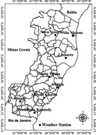
Reference evapotranspiration was estimated for eight locations in the state of Espírito Santo. Each site has an automatic gauge station from where data were gathered. The geographical location of these stations and respective cities to which they belong can be seen on the map in Figure 1. Table 1 contains information regarding the used automatic gauge stations that belong to the Brazilian Meteorological Institute (INMET).
The meteorological data used were respective to the period between 2007 and 2011. We used a data series relatively small for the stations being in operation only since 2006.
TABLE 1. Information regarding the weather stations used in the study.
INMET Code Location city Latitude Longitude Altitude (meters)
A617 Alegre -20º45’2.1” -41º29’20” 138
A615 Alfredo Chaves -20º38’11” -40º44’29” 35
A614 Linhares -19°21’24” -40°04’07” 40
A623 Nova Venécia -18º41’43” -40º23’26.8” 154 A622 Presidente Kennedy -21º06’4.3” -41º02’20” 80 A616 São Mateus -18º42’50” -39º50’53.8” 39 A613 Santa Teresa -19º59’19” -40º34’45.8” 998
A612 Vitória -20º18’56.1” -40º19’02” 9
FIGURE 1. Location of the automatic weather stations used in the study.
The reference evapotranspiration was estimated by the Penman-Monteith method – FAO-56, as stated by ALLEN et al. (1998), by means of the following equation:
in which,
is the reference evapotranspiration (mm d-1);
is the radiation balance (MJ m-2);
is the density of heat flow from the soil (MJ m-2);
is the mean air temperature (ºC);
is the wind speed at 2 meters above the soil (m s-1);
is the saturation vapor pressure (kPa);
is the partial vapor pressure (kPa);
is the slope of the saturation vapor pressure curve at a T temperature (kPa ºC-1),
is the psychrometric coefficient (kPa ºC-1).
Even though this method requires a great number of climatic elements, it has been widely used as scientific studies have proved its satisfactory performance when compared to lysimetric measurements (OLIVEIRA et al., 2008; BARROS et al., 2009; CAVALCANTE JUNIOR et al., 2011).
We assessed the following distributions: beta, gamma, generalized extreme value (GEV), generalized logistic (GLO), generalized normal (GN), Gumbel (G), normal (N), Pearson type 3 (P3), Weibull (W), two- and three-parameter lognormal (LN2 and LN3). These distributions are described by NAGHETTINI & PINTO (2007) and HOSKING (2013).
The probability density function of the gamma distribution is given by:
(2)
in which,
is the form parameter,
is the scale parameter, and
is the gamma function.
GEV distribution, with a location parameter , scale and form , has the following probability density function:
(3)
in which,
(4)
GLO probability density function with a location parameter , scale , form k, is given by:
(5)
in which,
GN distribution, with a location parameter , scale , form k, has the following probability density function:
(7) in which,
(8)
and
is the distribution function of the standard normal distribution.
Gumbel probability density function with a location parameter , scale , form k, is given by:
(9)
Normal probability density function is given by:
(10)
in which,
is the location parameter, and
is the scale one.
Pearson III distribution with parameters , and , is given by:
(11) in which,
(12)
Weibull distribution, with location parameter , scale , and form , has the following probability density function:
(13) Lognormal probability density function with parameters, and , is given by:
(14)
Lognormal probability density function with three parameters (a, and ) is given by:
Lastly, beta probability density function with parameters and is given by:
(16)
in which,
(17)
The parameters of the distributions were estimated by the L-moment method (HOSKING & WALLIS, 1997). MARTINS et al. (2011) stated that this method has been proposed to estimate parameters of the main probability distributions for hydrological studies.
ALVES et al. (2013) ascertained that the L-moment method estimates parameters of similar quality resulting from the maximum likelihood method.
The Kolmogorov-Smirnov a test was used to check the fit of the probability distributions to the ET0 data series (mm day-1), at 20% significance level. This level was chosen to make this hypothesis test stricter as an increase in significance level reduces the critical value of the test statistics. The test was performed by following the procedures described by NAGHETTINI & PINTO (2007).
Once the theoretical probability distribution with a good fit to the ET0 dataset was determined, a probable reference evapotranspiration was estimated as having probability inferior or equal to 75%, i.e. every four years on average. Therefore, the probable ET0 was reached or exceeded, at least once.
RESULTS AND DISCUSSION
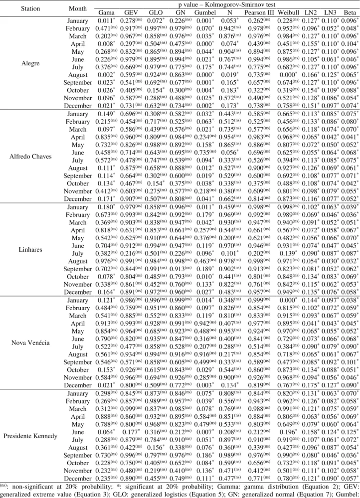
Table 2 show the results of the Kolmogorov-Smirnov good-fit test for the analyzed distributions, using “ns” for non-significant data at 20% probability (p > 0.20) and “*” for significant data at 20% (p < 0.20). Therefore, we noted that theoretical distributions with p-value above 0.20 had a good fit to the reference evapotranspiration dataset (ET0).
We might also see in Table 2 that GN distribution was the only that fitted to the ET0 dataset (mm day-1) for all studied months and locations. Furthermore, it is noteworthy that GEV, P3, GLO, and W distributions had also a good fit to ET0 dataset.
Conversely, gamma, normal, and Gumbel distributions showed a good fit for ET0 data series only in few months of the year, in the studied locations, whereas LN2 and LN3 probability distributions and beta presented no good fit to the dataset for any of the locations under study, as seen in Table 2.
In a study performed in Bahia state (Brazil), SILVA et al. (1998) observed that the best-fitted probability distributions to the ET0 data were normal, lognormal, and beta. Among the theoretical distributions analyzed by these authors, only the normal one fitted to ET0 data at certain times of the year, within the eight studied locations in the state of Espírito Santo (Table 2).
The GEV distribution fitted to the ET0 data series in virtually every month and sites, except for June and February in Presidente Kennedy and São Mateus, respectively. Likewise, GLO had a similar result to GEV (Table 2).
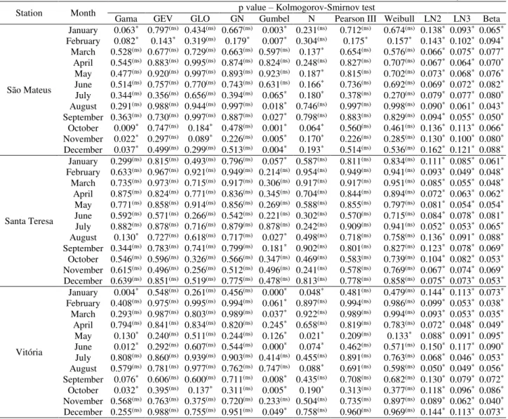
TABLE 2. Results of the Kolmogorov-Smirnov fitting test, at 20% significance, for the assessed probabilistic distributions.
Station Month p value – Kolmogorov-Smirnov test
Gama GEV GLO GN Gumbel N Pearson III Weibull LN2 LN3 Beta
Alegre
January 0.011* 0.278(ns) 0.072* 0.226(ns) 0.001* 0.053* 0.262(ns) 0.228(ns) 0.127* 0.110* 0.096* February 0.471(ns) 0.917(ns) 0.997(ns) 0.979(ns) 0.070* 0.942(ns) 0.978(ns) 0.952(ns) 0.096* 0.052* 0.048* March 0.202(ns) 0.967(ns) 0.858(ns) 0.976(ns) 0.035* 0.876(ns) 0.976(ns) 0.984(ns) 0.127* 0.110* 0.096* April 0.008* 0.297(ns) 0.504(ns) 0.475(ns) 0.000* 0.074* 0.439(ns) 0.451(ns) 0.155* 0.110* 0.104* May 0.268(ns) 0.832(ns) 0.865(ns) 0.894(ns) 0.044* 0.904(ns) 0.894(ns) 0.875(ns) 0.127* 0.110* 0.096* June 0.226(ns) 0.979(ns) 0.895(ns) 0.994(ns) 0.021* 0.767(ns) 0.994(ns) 0.986(ns) 0.105* 0.061* 0.046* July 0.376(ns) 0.669(ns) 0.979(ns) 0.775(ns) 0.175* 0.744(ns) 0.775(ns) 0.682(ns) 0.127* 0.110* 0.096* August 0.002* 0.595(ns) 0.924(ns) 0.863(ns) 0.000* 0.019* 0.735(ns) 0.000* 0.166* 0.125* 0.065* September 0.023* 0.541(ns) 0.692(ns) 0.677(ns) 0.001* 0.165* 0.657(ns) 0.674(ns) 0.127* 0.110* 0.096* October 0.026* 0.405(ns) 0.154* 0.300(ns) 0.004* 0.183* 0.322(ns) 0.319(ns) 0.154* 0.109* 0.088* November 0.096* 0.587(ns) 0.288(ns) 0.488(ns) 0.025* 0.572(ns) 0.490(ns) 0.521(ns) 0.128* 0.086* 0.054* December 0.021* 0.731(ns) 0.632(ns) 0.734(ns) 0.002* 0.173* 0.738(ns) 0.758(ns) 0.151* 0.097* 0.074*
Alfredo Chaves
January 0.149* 0.696(ns) 0.308(ns) 0.582(ns) 0.032* 0.443(ns) 0.585(ns) 0.665(ns) 0.113* 0.085* 0.075* February 0.215(ns) 0.454(ns) 0.717(ns) 0.525(ns) 0.063* 0.512(ns) 0.525(ns) 0.456(ns) 0.133* 0.086* 0.080* March 0.097* 0.586(ns) 0.439(ns) 0.576(ns) 0.021* 0.735(ns) 0.577(ns) 0.656(ns) 0.118* 0.074* 0.070* April 0.835(ns) 0.960(ns) 0.809(ns) 0.984(ns) 0.234(ns) 0.954(ns) 0.983(ns) 0.968(ns) 0.065* 0.042* 0.041* May 0.732(ns) 0.826(ns) 0.988(ns) 0.892(ns) 0.158* 0.865(ns) 0.886(ns) 0.807(ns) 0.072* 0.050* 0.052* June 0.458(ns) 0.714(ns) 0.643(ns) 0.695(ns) 0.735(ns) 0.056* 0.696(ns) 0.625(ns) 0.055* 0.064* 0.068* July 0.572(ns) 0.478(ns) 0.747(ns) 0.539(ns) 0.094* 0.333(ns) 0.526(ns) 0.394(ns) 0.113* 0.085* 0.075* August 0.111* 0.875(ns) 0.658(ns) 0.888(ns) 0.012* 0.527(ns) 0.900(ns) 0.927(ns) 0.126* 0.069* 0.061* September 0.114* 0.664(ns) 0.302(ns) 0.600(ns) 0.019* 0.529(ns) 0.600(ns) 0.692(ns) 0.108* 0.077* 0.071* October 0.134* 0.467(ns) 0.154* 0.375(ns) 0.038* 0.338(ns) 0.375(ns) 0.488(ns) 0.108* 0.074* 0.042* November 0.412(ns) 0.603(ns) 0.275(ns) 0.577(ns) 0.218(ns) 0.380(ns) 0.609(ns) 0.801(ns) 0.098* 0.079* 0.055* December 0.171* 0.907(ns) 0.507(ns) 0.808(ns) 0.041* 0.662(ns) 0.814(ns) 0.873(ns) 0.116* 0.077* 0.052*
Linhares
January 0.180* 0.979(ns) 0.858(ns) 0.996(ns) 0.011* 0.459(ns) 0.998(ns) 0.998(ns) 0.102* 0.063* 0.039* February 0.673(ns) 0.993(ns) 0.842(ns) 0.992(ns) 0.179* 0.969(ns) 0.992(ns) 0.989(ns) 0.069* 0.046* 0.036* March 0.369(ns) 0.903(ns) 0.838(ns) 0.947(ns) 0.042* 0.930(ns) 0.947(ns) 0.940(ns) 0.091* 0.052* 0.051* April 0.818(ns) 0.631(ns) 0.853(ns) 0.661(ns) 0.257(ns) 0.544(ns) 0.661(ns) 0.567(ns) 0.072* 0.058* 0.067* May 0.542(ns) 0.625(ns) 0.910(ns) 0.644(ns) 0.376(ns) 0.200(ns) 0.621(ns) 0.482(ns) 0.056* 0.066* 0.070* June 0.704(ns) 0.912(ns) 0.994(ns) 0.947(ns) 0.119* 0.970(ns) 0.946(ns) 0.931(ns) 0.074* 0.047* 0.045* July 0.382(ns) 0.216(ns) 0.501(ns) 0.226(ns) 0.096* 0.101* 0.202(ns) 0.139* 0.090* 0.087* 0.087* August 0.976(ns) 0.991(ns) 0.984(ns) 0.998(ns) 0.463(ns) 0.978(ns) 0.998(ns) 0.971(ns) 0.054* 0.030* 0.032* September 0.702(ns) 0.844(ns) 0.991(ns) 0.913(ns) 0.189* 0.902(ns) 0.913(ns) 0.823(ns) 0.081* 0.052* 0.062* October 0.078* 0.804(ns) 0.485(ns) 0.793(ns) 0.010* 0.441(ns) 0.801(ns) 0.848(ns) 0.134* 0.083* 0.069* November 0.338(ns) 0.861(ns) 0.452(ns) 0.760(ns) 0.133* 0.822(ns) 0.761(ns) 0.842(ns) 0.115* 0.062* 0.053* December 0.164* 0.891(ns) 0.972(ns) 0.960(ns) 0.027* 0.483(ns) 0.957(ns) 0.949(ns) 0.135* 0.076* 0.058*
Nova Venécia
January 0.121* 0.986(ns) 0.996(ns) 0.999(ns) 0.014* 0.348(ns) 0.999(ns) 0.000* 0.144* 0.097* 0.038* February 0.484(ns) 0.759(ns) 0.951(ns) 0.860(ns) 0.097* 0.826(ns) 0.854(ns) 0.815(ns) 0.102* 0.072* 0.059* March 0.541(ns) 0.885(ns) 0.552(ns) 0.833(ns) 0.119* 0.810(ns) 0.833(ns) 0.915(ns) 0.093* 0.067* 0.059* April 0.913(ns) 0.993(ns) 0.928(ns) 0.991(ns) 0.942(ns) 0.407(ns) 0.977(ns) 0.895(ns) 0.041* 0.043* 0.045* May 0.854(ns) 0.964(ns) 0.685(ns) 0.923(ns) 0.488(ns) 0.953(ns) 0.924(ns) 0.970(ns) 0.065* 0.055* 0.052* June 0.790(ns) 0.820(ns) 0.935(ns) 0.847(ns) 0.316(ns) 0.400(ns) 0.841(ns) 0.729(ns) 0.073* 0.066* 0.068* July 0.522(ns) 0.477(ns) 0.858(ns) 0.528(ns) 0.207(ns) 0.288(ns) 0.514(ns) 0.384(ns) 0.090* 0.079* 0.090* August 0.561(ns) 0.934(ns) 0.994(ns) 0.916(ns) 0.916(ns) 0.217(ns) 0.854(ns) 0.718(ns) 0.065* 0.061* 0.067* September 0.546(ns) 0.571(ns) 0.858(ns) 0.605(ns) 0.499(ns) 0.333(ns) 0.589(ns) 0.477(ns) 0.085* 0.092* 0.101* October 0.153* 0.926(ns) 0.615(ns) 0.843(ns) 0.029* 0.544(ns) 0.860(ns) 0.873(ns) 0.134* 0.088* 0.051* November 0.584(ns) 0.966(ns) 0.694(ns) 0.926(ns) 0.285(ns) 0.900(ns) 0.926(ns) 0.968(ns) 0.094* 0.056* 0.046* December 0.021* 0.800(ns) 0.509(ns) 0.772(ns) 0.003* 0.134* 0.819(ns) 0.767(ns) 0.175* 0.127* 0.090*
Presidente Kennedy
TABLE 2. Results of the Kolmogorov-Smirnov fitting test, at 20% significance, for the assessed probabilistic distributions.
(Continuation)
Station Month p value – Kolmogorov-Smirnov test
Gama GEV GLO GN Gumbel N Pearson III Weibull LN2 LN3 Beta
São Mateus
January 0.063* 0.797(ns) 0.434(ns) 0.667(ns) 0.003* 0.231(ns) 0.712(ns) 0.674(ns) 0.138* 0.093* 0.065* February 0.082* 0.143* 0.319(ns) 0.179* 0.007* 0.304(ns) 0.175* 0.157* 0.143* 0.102* 0.094* March 0.528(ns) 0.677(ns) 0.729(ns) 0.663(ns) 0.597(ns) 0.137* 0.654(ns) 0.576(ns) 0.066* 0.075* 0.077* April 0.545(ns) 0.883(ns) 0.995(ns) 0.874(ns) 0.824(ns) 0.248(ns) 0.827(ns) 0.707(ns) 0.067* 0.064* 0.070* May 0.477(ns) 0.920(ns) 0.997(ns) 0.893(ns) 0.923(ns) 0.187* 0.815(ns) 0.702(ns) 0.073* 0.068* 0.076* June 0.514(ns) 0.757(ns) 0.770(ns) 0.743(ns) 0.631(ns) 0.166* 0.736(ns) 0.692(ns) 0.069* 0.072* 0.082* July 0.344(ns) 0.356(ns) 0.656(ns) 0.394(ns) 0.065* 0.180* 0.378(ns) 0.270(ns) 0.079* 0.077* 0.080* August 0.291(ns) 0.988(ns) 0.944(ns) 0.997(ns) 0.018* 0.746(ns) 0.997(ns) 0.998(ns) 0.090* 0.061* 0.043* September 0.363(ns) 0.730(ns) 0.997(ns) 0.887(ns) 0.027* 0.798(ns) 0.883(ns) 0.829(ns) 0.094* 0.055* 0.050* October 0.009* 0.747(ns) 0.184* 0.478(ns) 0.001* 0.064* 0.560(ns) 0.461(ns) 0.136* 0.113* 0.066* November 0.022* 0.297(ns) 0.089* 0.226(ns) 0.005* 0.170* 0.226(ns) 0.285(ns) 0.130* 0.100* 0.080* December 0.037* 0.499(ns) 0.299(ns) 0.513(ns) 0.004* 0.193* 0.514(ns) 0.536(ns) 0.162* 0.121* 0.088*
Santa Teresa
January 0.299(ns) 0.815(ns) 0.493(ns) 0.796(ns) 0.057* 0.587(ns) 0.811(ns) 0.834(ns) 0.111* 0.085* 0.061* February 0.633(ns) 0.967(ns) 0.921(ns) 0.949(ns) 0.214(ns) 0.954(ns) 0.949(ns) 0.941(ns) 0.093* 0.049* 0.048* March 0.735(ns) 0.973(ns) 0.715(ns) 0.917(ns) 0.306(ns) 0.917(ns) 0.917(ns) 0.951(ns) 0.085* 0.055* 0.048* April 0.875(ns) 0.824(ns) 0.771(ns) 0.836(ns) 0.345(ns) 0.704(ns) 0.844(ns) 0.894(ns) 0.072* 0.063* 0.062* May 0.771(ns) 0.858(ns) 0.914(ns) 0.856(ns) 0.269(ns) 0.588(ns) 0.855(ns) 0.797(ns) 0.081* 0.054* 0.054* June 0.592(ns) 0.571(ns) 0.266(ns) 0.542(ns) 0.221(ns) 0.302(ns) 0.570(ns) 0.715(ns) 0.084* 0.078* 0.081* July 0.882(ns) 0.878(ns) 0.716(ns) 0.879(ns) 0.878(ns) 0.242(ns) 0.909(ns) 0.941(ns) 0.052* 0.053* 0.065* August 0.130* 0.727(ns) 0.618(ns) 0.717(ns) 0.027* 0.498(ns) 0.718(ns) 0.758(ns) 0.136* 0.091* 0.088* September 0.344(ns) 0.783(ns) 0.741(ns) 0.799(ns) 0.181* 0.902(ns) 0.801(ns) 0.827(ns) 0.123* 0.078* 0.069* October 0.546(ns) 0.596(ns) 0.326(ns) 0.566(ns) 0.347(ns) 0.469(ns) 0.583(ns) 0.739(ns) 0.104* 0.082* 0.053* November 0.615(ns) 0.496(ns) 0.256(ns) 0.512(ns) 0.496(ns) 0.241(ns) 0.578(ns) 0.769(ns) 0.067* 0.074* 0.069* December 0.639(ns) 0.851(ns) 0.519(ns) 0.775(ns) 0.478(ns) 0.813(ns) 0.778(ns) 0.858(ns) 0.075* 0.073* 0.053*
Vitória
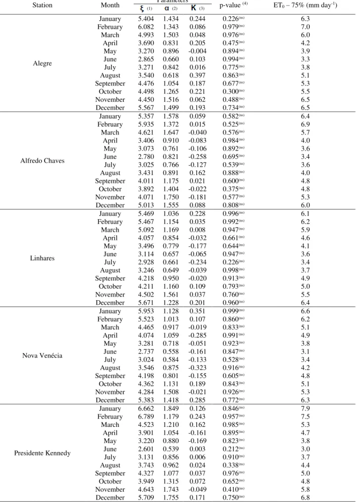
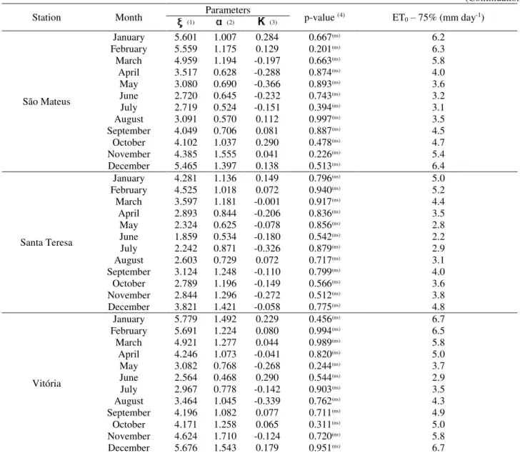
TABLE 3. Parameters of the generalized normal distribution (GN), KS test p-value and estimated ET0 at 75% probability for the studied stations.
Station Month Parameters p-value (4) ET
0– 75% (mm day-1) (1) (2) (3)
Alegre
January 5.404 1.434 0.244 0.226(ns) 6.3 February 6.082 1.343 0.086 0.979(ns) 7.0 March 4.993 1.503 0.048 0.976(ns) 6.0 April 3.690 0.831 0.205 0.475(ns) 4.2 May 3.270 0.896 -0.004 0.894(ns) 3.9 June 2.865 0.660 0.103 0.994(ns) 3.3 July 3.271 0.842 0.016 0.775(ns) 3.8 August 3.540 0.618 0.397 0.863(ns) 5.1 September 4.476 1.054 0.187 0.677(ns) 5.3 October 4.498 1.265 0.221 0.300(ns) 5.5 November 4.450 1.516 0.062 0.488(ns) 6.5 December 5.567 1.499 0.193 0.734(ns) 6.5
Alfredo Chaves
January 5.357 1.578 0.059 0.582(ns) 6.4 February 5.935 1.372 0.015 0.525(ns) 6.9 March 4.621 1.647 -0.040 0.576(ns) 5.7 April 3.406 0.910 -0.083 0.984(ns) 4.0 May 3.073 0.761 -0.106 0.892(ns) 3.6 June 2.780 0.821 -0.258 0.695(ns) 3.4 July 3.025 0.766 -0.127 0.539(ns) 3.6 August 3.431 0.891 0.162 0.888(ns) 4.0 September 4.011 1.175 0.021 0.600(ns) 4.8 October 3.892 1.404 -0.022 0.375(ns) 4.8 November 4.071 1.750 -0.181 0.577(ns) 5.3 December 5.013 1.555 0.088 0.808(ns) 6.0
Linhares
January 5.469 1.036 0.228 0.996(ns) 6.1 February 5.467 1.154 0.035 0.992(ns) 6.2 March 5.092 1.169 0.008 0.947(ns) 5.9 April 4.057 0.854 -0.032 0.661(ns) 4.6 May 3.496 0.779 -0.177 0.644(ns) 4.1 June 3.114 0.657 -0.065 0.947(ns) 3.6 July 2.928 0.661 -0.234 0.226(ns) 3.4 August 3.246 0.649 -0.039 0.998(ns) 3.7 September 4.218 0.950 -0.020 0.913(ns) 4.9 October 4.211 1.160 0.109 0.793(ns) 5.0 November 4.502 1.561 0.037 0.760(ns) 5.5 December 5.671 1.228 0.201 0.960(ns) 6.4
Nova Venécia
January 5.953 1.128 0.351 0.999(ns) 6.6 February 5.523 1.013 0.107 0.860(ns) 6.2 March 4.465 0.917 -0.019 0.833(ns) 5.1 April 4.074 1.059 -0.285 0.991(ns) 4.9 May 3.281 0.718 -0.051 0.923(ns) 3.8 June 2.737 0.558 -0.161 0.847(ns) 3.1 July 3.024 0.584 -0.133 0.528(ns) 3.4 August 3.546 0.875 -0.323 0.916(ns) 4.2 September 4.198 0.801 -0.155 0.605(ns) 4.8 October 4.362 1.131 0.189 0.843(ns) 5.1 November 4.284 1.508 -0.021 0.926(ns) 5.3 December 5.383 1.418 0.285 0.772(ns) 6.3
Presidente Kennedy
TABLE 3. Parameters of the generalized normal distribution (GN), KS test p-value and estimated ET0 at 75% probability for the studied stations.
(Continuation)
Station Month Parameters p-value (4) ET
0– 75% (mm day-1) (1) (2) (3)
São Mateus
January 5.601 1.007 0.284 0.667(ns) 6.2 February 5.559 1.175 0.129 0.201(ns) 6.3 March 4.959 1.194 -0.197 0.663(ns) 5.8 April 3.517 0.628 -0.288 0.874(ns) 4.0 May 3.080 0.690 -0.366 0.893(ns) 3.6 June 2.720 0.645 -0.232 0.743(ns) 3.2 July 2.719 0.524 -0.151 0.394(ns) 3.1 August 3.091 0.570 0.112 0.997(ns) 3.5 September 4.049 0.706 0.081 0.887(ns) 4.5 October 4.102 1.037 0.290 0.478(ns) 4.7 November 4.385 1.555 0.041 0.226(ns) 5.4 December 5.465 1.397 0.138 0.513(ns) 6.4
Santa Teresa
January 4.281 1.136 0.149 0.796(ns) 5.0 February 4.525 1.018 0.072 0.940(ns) 5.2 March 3.597 1.181 -0.001 0.917(ns) 4.4 April 2.893 0.844 -0.206 0.836(ns) 3.5 May 2.324 0.625 -0.078 0.856(ns) 2.8 June 1.859 0.534 -0.180 0.542(ns) 2.2 July 2.242 0.871 -0.326 0.879(ns) 2.9 August 2.603 0.729 0.072 0.717(ns) 3.1 September 3.124 1.248 -0.110 0.799(ns) 4.0 October 2.789 1.196 -0.149 0.566(ns) 3.6 November 2.844 1.296 -0.272 0.512(ns) 3.8 December 3.821 1.421 -0.058 0.775(ns) 4.8
Vitória
January 5.779 1.492 0.229 0.456(ns) 6.7 February 5.691 1.224 0.080 0.994(ns) 6.5 March 4.921 1.277 0.044 0.989(ns) 5.8 April 4.246 1.073 -0.041 0.820(ns) 5.0 May 3.082 0.768 -0.268 0.244(ns) 3.7 June 2.564 0.468 0.290 0.544(ns) 2.9 July 2.967 0.778 -0.142 0.903(ns) 3.5 August 3.464 1.045 -0.339 0.762(ns) 4.3 September 4.196 1.082 0.077 0.711(ns) 4.9 October 4.171 1.258 0.065 0.311(ns) 5.0 November 4.624 1.710 -0.124 0.720(ns) 5.8 December 5.676 1.543 0.179 0.951(ns) 6.7
(ns): non-significant at 20% probability by the Kolmogorov-Smirnov test; (1) Location parameter; (2) Scale parameter; and (3) Form parameter.
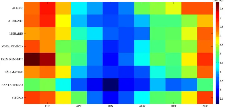
Figure 2 shows the ET0 variation estimated at 75% probability throughout the year. An analysis of the graph in Figure 2 showed that the higher ET0 rates occur from December to February (from 4.8 to 7.9 mm day-1), while the lowest ones are between May and July (from 2.2 to 4.1 mm dia-1) (Table 3). It is noteworthy that the highest ET
FIGURE 2. Variation in the reference evapotranspiration estimated on generalized normal distribution (GN) at 75% probability during the year
In the months of March, April, August, September, and October, ET0 estimated at 75% probability ranged from 3.1 to 6.0 mm day -1 (Table 3).
The highest value of ET0 was recorded in January, in Presidente Kennedy (7.9 mm day-1). This outcome was already expected since this area has high wind speeds and temperatures. On the other side, the lowest values were registered in the city of Santa Teresa, located in the highlands of the state.
In light of the role played by the management of water resources in irrigated farming, all the information shown in Table 3, as well as ET0 behavior throughout the year, are fundamental for estimation of effective irrigation intervals and applied water depth, avoiding irrigation water waste (MANTOVANI et al., 2009).
In this study, we have solely estimated ET0 rates at 75% probability; however, making use of the parameters of a generalized normal distribution, shown in Table 3, we can estimate it at other probability levels, enabling the draughtsman to choose a proper degree of risk.
CONCLUSIONS
The Generalized Normal, Generalized Extreme Values, Pearson III, Generalized Logistics, and Weibull distributions showed a good fit to the ET0 data, with Generalized Normal being the one that properly described the data (in mm day-1) for all the months and locations under study in the state of Espírito Santo (Brazil).
Continuous probability models can be used to estimate daily reference evapotranspiration associated with a certain level of risk, allowing the acquisition of probable ET0 data for irrigation system sizing purposes.
ACKNOWLEDGEMENTS
REFERENCES
ALLEN, R.G.; PEREIRA, L.S.; RAES, D.; SMITH, M. Crop evapotranspiration: guidelines for computing crop water requirements. Rome: FAO, 1998. 300p. (Irrigation and Drainage Paper, 56).
ALVES, A.V.P.; SANTOS, G.B.S.; MENEZES FILHO, F.C.M.; SANCHES, L. Análise dos Métodos de Estimativa para os Parâmetros das Distribuições de Gumbel e GEV em Eventos de Precipitações Máximas na Cidade de Cuiabá‐MT. Revista Eletrônica de Engenharia Civil, Goiânia, v. 6, n. 1, p.32-43, 2013.
ASSIS, J. P.; SOUSA, R. P.; BEZERRA NETO, F.; LINHARES, P. C. F. Tables of probabilities of reference evapotranspiration for the region of Mossoró, RN, Brazil. Revista Verde de
Agroecologia e Desenvolvimento Sustentável, Pombal, v. 9, n. 3, p.58-67, 2014.
BARROS, V.R.; SOUZA, A.P.; FONSECA, D.C.; SILVA, L.B.D. Avaliação da evapotranspiração de referência na Região de Seropédica, Rio de Janeiro, utilizando lisímetro de pesagem e modelos matemáticos. Revista Brasileira de Ciências Agrárias, Recife, v. 4, n. 2, p.198-203, 2009.
BERNARDO, S; SOARES, A. A.; MANTOVANI, E. C. Manual de
Irrigação. Viçosa: UFV, 2006. 625 p.
CAVALCANTE JUNIOR, E.G.; OLIVEIRA, A.D.; ALMEIDA, B.M.; SOBRINHO, J. E. Métodos de estimativa da evapotranspiração de referência para as condições do semiárido
Nordestino. Semina: Ciências Agrárias, Londrina, v. 32, n. 1, p.1699-1708, 2011.
HOSKING, J.R.M. Package ‘lmom’. Disponível em: <http://cran.r-project.org/web/packages/
lmom/lmom.pdf>. Acesso em: 02 jul 2013.
HOSKING, J. R. M.; WALLIS, J. R. Regional frequency analysis: an approach based on L-moments. Cambridge: Cambridge University Press, 1997. 224 p.
MANTOVANI, E.C.; BERNARDO, S.; PALARETTI, L.F. Irrigação: princípios e métodos. 3. ed. Viçosa: UFV, 2009. 355 p.
MARTINS, C.A.S.; ULIANA, E.M.; REIS, E.F. Estimativa da Vazão e da Precipitação Máxima utilizando Modelos Probabilísticos na Bacia Hidrográfica do Rio Benevente. Enciclopédia
Biosfera, Goiânia, v. 7, n. 13, p.1130-1142, 2011.
NAGUETTINI, M.; PINTO, E. J. A. Hidrologia estatística. Belo Horizonte: CPRM, 2007. 552 p.
OLIVEIRA, L.M.M.; MONTENEGRO, S.M.G.L.; AZEVEDO, J.R.G.; SANTOS, F.X. Evapotranspiração de referência na bacia experimental do riacho Gameleira, PE, utilizando-se lisímetro e métodos indiretos. Revista Brasileira de Ciências Agrárias, Recife, v. 3, n. 1, p.58-67, 2008.
SAAD, J.C.C.; BISCARO, G.A.; DELMANTO JUNIOR, O.; FRIZZONE, J.A. Estudo da Distribuição da Evapotranspiração de Referência Visando o Dimensionamento de Sistemas de Irrigação. Irriga, Botucatu, v. 1, n. 7, p.10-17, 2002.
SILVA, F.C.; FIETZ, C.R.; FOLEGATTI, M.V.; PEREIRA, F.A.C. Distribuição e Frequência da Evapotranspiração de Referência de Cruz das Almas, BA. Revista Brasileira de Engenharia
Agrícola e Ambiental, Campina Grande, v. 2, n. 3, p.284-286, 1998.