Process Safety and Environmental Protection 1 0 2 ( 2 0 1 6 )263–276
Contents lists available atScienceDirect
Process Safety and Environmental Protection
j o u r n a l h o m e p a g e :w w w . e l s e v i e r . c o m / l o c a t e / p s e p
Fish canning industry wastewater variability
assessment using multivariate statistical methods
Raquel O. Cristóvão
a,∗, Victor M.S. Pinto
b, António Gonc¸alves
c,
Ramiro J.E. Martins
a,b, José M. Loureiro
a, Rui A.R. Boaventura
aaLaboratory of Separation and Reaction Engineering (LSRE), Associate Laboratory LSRE/LCM, Department of
Chemical Engineering, Faculty of Engineering, University of Porto, Rua do Dr. Roberto Frias, 4200-465 Porto, Portugal
bDepartment of Chemical and Biological Technology, Superior School of Technology, Polytechnic Institute of
Braganc¸a, Campus de Santa Apolónia, 5301-857 Braganc¸a, Portugal
cCRACS/INESC-TEC and Department of Computer Science, Faculty of Sciences, University of Porto, Rua do Campo
Alegre 1021/1055, 4169-007 Porto, Portugal
a r t i c l e
i n f o
Article history:
Received 26 October 2015 Received in revised form 18 March 2016
Accepted 24 March 2016 Available online 1 April 2016
Keywords:
Fish canning wastewater Wastewater variability Principal component analysis Cluster analysis
Correlation analysis
Multivariate statistical methods
a b s t r a c t
Usually, fish canning industrial wastewaters have a highly variable composition over time. For a good performance of treatment processes it is necessary to limit that variation. However, extended wastewater monitoring, including all relevant analytical parameters, is expensive. This work proposes an efficient approach to minimize the analytical determina-tions number without compromising the global characterization goal. This way, fish canning industry wastewaters variability was assessed and interpreted through multivariate statis-tical tools application to analystatis-tical data obtained from a monitoring program carried out in a fish canning industry of northern Portugal. 23 physicochemical parameters were determined in 20 samples collected on an 8 months period. The results achieved by correlation analysis, principal component analysis (PCA) and cluster analysis (CA) led to the main water pollu-tion sources identificapollu-tion and to the minimizapollu-tion of physical and chemical parameters number to be analyzed in order to achieve a correct wastewater characterization, at mini-mum cost. The main pollution sources proved to be the brine and eviscerating step waters. Dissolved organic carbon (DOC), total suspended solids (TSS), conductivity, pH, Ca2+, F−and
one of the parameters SO42, NO3−and PO43−were identified as important parameters that
must be monitored in order to obtain an accurate characterization allowing to define the most appropriate wastewater treatment.
© 2016 The Institution of Chemical Engineers. Published by Elsevier B.V. All rights reserved.
1.
Introduction
In recent years, there has been a rapid growth of commer-cial fish markets and industries across the world. Countries with rapid population, income and urbanization growths tend to have the greatest increases of fish products consumption (Delgado et al., 2003). The volume and concentration of waste-water produced by fish canning industries is highly variable, depending on the production season, fish type that is being
∗ Corresponding author. Tel.: +351 22 508 2263; fax: +351 22 508 1674.
E-mail address:[email protected](R.O. Cristóvão).
processed, additives used, processing water source and on the unit processes implemented (Chowdhury et al., 2010). Each plant is unique, so generalizations about water use and waste-water characteristics are difficult.
The treatment of these effluents is complex due to the pres-ence of high content of organic matter, oil and grease and also due to the high NaCl concentration that they normally present (Cristóvão et al., 2015; Gharsallah et al., 2002). Cur-rently most of fish canning industries in Portugal only perform
http://dx.doi.org/10.1016/j.psep.2016.03.016
264
Process Safety and Environmental Protection 1 0 2 ( 2 0 1 6 ) 263–276a pre-treatment of their wastewaters, usually by screening, fil-tration and/or decanting to remove coarse particles (Cristóvão et al., 2014). However, there is a need to consider the treatment of these wastewaters in order to fulfil the limits imposed by the Portuguese legislation (Decree-Law No. 236/98) for indus-trial wastewater discharge. The overall treatment efficiency varies according to wastewater characteristics and with the technologies applied. Since the wastewaters from fish can-ning industrial processes are known to have a high variability, there is a need to know their characteristics in detail in order to decide the best treatment sequence to apply. In fact, for a good performance of certain treatment processes (i.e., to obtain a good efficiency) it is necessary to limit wastewater variation. The usual manner of achieving this is to install a homogenizing tank upstream from the treatment system. For the homogenization tank design it is essential to know the wastewater analytical parameters with higher variabil-ity (or that contribute most to the overall variabilvariabil-ity of the effluent). Knowing these parameters it is possible, for a given level of probability, to calculate the residence time in the homogenization tank (and, therefore, the volume, assuming an approximately constant flow rate) so that the concentra-tions of the output parameters are within a predefined range. This could be achieved with the design of monitoring pro-grams for collection of different wastewater samples before being launched to the wastewater treatment plant (WWTP) and subsequent characterization of a large number of physi-cochemical parameters to provide representative and reliable wastewater quality parameters. However, these programs are expensive and produce large data sets which are often difficult to analyze and interpret. In these cases, the use of multivariate statistical analysis methods is appealing.
Multivariate statistical methods are useful for the inter-pretation of large and complex water and wastewater quality data sets, evaluating redundant measurements in the environ-ment, allowing, this way, the classification and the grouping of pollutants according to their sources, achieving a small num-ber of underlying factors without losing too much information (Singh et al., 2005). Correlation analysis is a well-known statis-tical method to assess the relationships between parameters. The resulting value, the correlation coefficient, can range between ±1 and shows if the variation of one variable is correlated to the variation of other variable. The closer the cor-relation is to +1 or−1, the closer it is to a perfect relationship (Babu et al., 2014). Although useful, sometimes correlation analysis leads to a large number of variables that are difficult to examine and the correlations between the variables can be better observed and qualitatively visualized using cluster analysis. CA is a classification method used to split a data set into a number of groups of observations that share observed properties and are distinct from each other in terms of vari-ables values (Paoletti et al., 2002). There are different clustering techniques, but hierarchical agglomerative clustering is the most important and widely used. In clustering, the objects are grouped such that similar objects fall into the same class (cluster). The hierarchical agglomerative clustering is based on distances between clusters. Given an initial cluster, first the two clusters that are nearest are merged to form a new cluster. This is repeated each time merging the two closest clusters, until just one cluster, of all the data points, exists. The lev-els of similarity at which observations are merged are used to construct a dendrogram (Hand et al., 2001; Magyar et al., 2013). A third data analysis method, principal components analysis, can also be used to explore the relationships among several
samples, being at the same time, a variable reduction proce-dure. PCA is a statistical technique that transforms the original set of inter-correlated variables into a new set with a small number of independent uncorrelated variables or principal components (PCs) that are linear combinations of the original variables and account for most of the variance in the observed variables. This way, principal components do not present mul-ticollinearity probably present in original variables (Hatcher and Stepansku, 1994; Song et al., 2006). The aim of this tech-nique is to capture the intrinsic variability in the data and to identify groups of variables based on the loadings (the weight by which each standardized original variable should be mul-tiplied to get the component score), i.e., correlations between the variables and the principal components (Boruvka et al., 2005). Loadings show how well a variable is taken into account by the model components and can be used to understand how much each variable contributes to the meaningful variation in the data and to interpret variable relationships. Loadings are also useful for interpreting the meaning of each compo-nent. This is a useful way of reducing the dimensionality of a data set, either to ease interpretation or as a way to avoid overfitting and to prepare for subsequent analysis (Hand et al., 2001).
Using correlation analysis with CA and PCA provides more information than using each method alone. These multivariate statistical analyses can be efficient tools for evaluating water/wastewater quality and also for identifying latent sources that influence their characteristics, reducing the dimensionality of a data set and offering a valuable tool for reliable management of water resources, as well as effective solutions to pollution problems (Magyar et al., 2013; Lee et al., 2008; Ouali et al., 2009; Wan et al., 2011; Wang et al., 2013; Yoo et al., 2003; Zhao et al., 2012).
In this work, correlation analysis, PCA and CA were per-formed to analyze data from twenty different wastewater samples resulting from a sampling program carried out in a fish canning industry of northern Portugal, from November 2013 to June 2014, aiming at assessing linear relationships between wastewater characterization parameters and to eval-uate main wastewater pollution sources in order to optimize and reduce the number of monitoring parameters (redun-dant and correlated information), preserving the maximum of information whereas minimizing the analysis costs.
2.
Materials and methods
2.1. Fish canning industry process
Process Safety and Environmental Protection 1 0 2 ( 2 0 1 6 ) 263–276
265
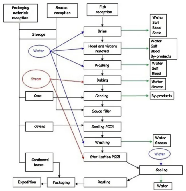
Fig. 1 – Fish canning industry flowchart (Cristóvão et al., 2012).
2.2. Wastewater samples collection and
characterization
To study the fish canning wastewater characterization and its variability, a sampling program was carried out in a selected fish canning industry of northern Portugal. Twenty samples were taken from the final common well at different time periods (from November 2013 to June 2014) and were char-acterized in terms of physicochemical parameters. Three sampling types were previously defined. In the first 4 months about 12 spot wastewater samples were collected: two sam-ples of 10 L each per day, one in the morning, usually between 10 and 10:30 AM, and another one in the afternoon, between 4 and 4:30 PM. In the final 3 months, 7 daily composed sam-ples and 1 weekly composed sample were collected. Daily composed samples were prepared by spot samples addition collected every 2 h between 9:30 AM and 5:30 PM (correspond-ing to 8 h of a work(correspond-ing day), mak(correspond-ing a total of 10 L. The weekly composed sample was prepared by daily effluent collection every 2 h, between 9:30 AM and 5:30 PM, making a daily total volume of 5 L. At the end of the week, 2 L were removed from each of the five daily composed samples and mixed in another container, representing the final weekly sample.
Standard Methods for the Examination of Water and Wastewater (APHA, 2005) were used for the measurement of total suspended solids (TSS), volatile suspended solids (VSS), dissolved organic carbon (DOC), chemical oxygen demand (COD), biological oxygen demand (BOD), oil and grease (O&G), total phosphorus (Ptotal), total soluble nitrogen (Ntotal soluble) and several anions and cations. For DOC measurements a Shi-madzu 5000A Total Organic Carbon analyzer was used. The values reported represent the average of at least two measure-ments; in most cases each sample was injected three times, validation being performed by the apparatus only if the coef-ficient of variation (CV) was smaller than 2%.
The pH was measured using a selective electrode (Hanna Instruments HI 1230) and a pH meter (Hanna instruments HI 8424) and the conductivity at 20◦C was determined using a conductivity probe (WTW TetraCon 325) and a conductivity meter (WTW LF538).
266
Process Safety and Environmental Protection 1 0 2 ( 2 0 1 6 ) 263–276NaOH 30 mM/methanesulfonic acid 20 mM at a flow rate of 1.5/1.0 mL/min for anions/cations analysis, respectively.
2.3. Multivariate statistical analysis
2.3.1. Correlation analysis
The linear relationship between the studied parameters val-ues can be evaluated through the correlation coefficients between those values in the different samples. Correlation analysis was performed according to Pearson Product Moment Correlation (Eq.(1)) (Anderson, 1996) using a R multivariate data analysis software package.
r=rxy=
ni=1(xi−x¯)(yi−y¯)
ni=1(xi−x¯)2
ni=1(yi−y¯)2
(1)
wherenis the total number of values in a dataset,xiare the values inside a datasetx,yiare the values inside a datasety, ¯x
is the sample mean of datasetxand ¯yis the sample mean of datasety.
The correlation coefficient between two parameters is found where a given row and column intersect in the correla-tion matrix. A coefficient of +1.0, a perfect positive correlacorrela-tion, means that changes in the first variable will result in a positive change in the second variable. A coefficient of−1.0, a perfect negative correlation, means that changes in the first variable will result in an identical change in the second variable, but the change will be in the opposite direction. A coefficient of zero means that there is no relationship between the two variables and that a change in the first variable will have no effect in the second one (Jackson, 2002).
To evaluate the statistical significance of correlations, the possible correlation coefficients should be compared with a calculated critical coefficient that should have at least a sig-nificance level of 0.05, which means that the confidence level that they are not random chance results is at least 95% (Pires et al., 2008). The selection of the correlation coefficients will be based on a threshold of at least 0.7 as this is the minimum for having a strong dependency between two variables.
2.3.2. Cluster analysis (CA)
Cluster analysis is used to group objects based on the simi-larity between them, i.e., to group variables with the highest correlations. In this study, a hierarchical agglomeration algo-rithm for clustering was performed using a R multivariate data analysis software package and the distances (or correlations) between all samples were calculated using a defined metric, the Euclidean distance. The applied clustering procedure was the Average Linkage Method. Initially, each object is assigned to its own cluster and then the algorithm proceeds iteratively, at each stage joining the two most similar clusters, continu-ing until there is just a scontinu-ingle cluster. At each stage distances between clusters are recomputed by the Lance–Williams dis-similarity update formula according to the clustering method. Finally, a graphic (dendrogram) that displays how the samples are clustered is produced. The clusters are assembled using all the variance in the dataset.
2.3.3. Principal component analysis (PCA)
PCA is a multivariate data analysis technique that uses an orthogonal transformation of the original possibly correlated variables (almost always correlated) to project them onto a smaller number of uncorrelated variables called principal
components. The first principal component explains most of the variation in the data. The second principal component is orthogonal to the first and covers as much of the remaining variation as possible, and so on (Abdul-Wahab et al., 2005; Viana et al., 2006).
There are several criteria for the selection of number of PCs to retain) (Hatcher and Stepansku, 1994):
1. Retain principal components describing at least 70% of the total variance;
2. Retain principal components whose eigenvalues are higher than 1 –Kaiser criterion (Kaiser, 1960);
3. Plot a graph of variance vs principal components – scree test (Cattell, 1966) – and look for a “break” or an “elbow” between the components with relatively large variances and those with small. The components that appear before the break are assumed to be meaningful.
By plotting the principal components in a biplot, it is also possible to view inter-relationships between different param-eters and detect and interpret sample patterns, groupings, similarities or differences (Kara, 2009).
In this study, the PCA was performed using a R multivariate data analysis software package.
3.
Results and discussion
3.1. Analysis of wastewaters from fish canning industries
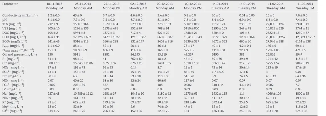
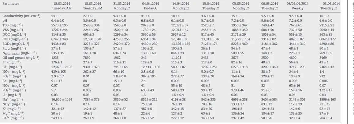
The fish canning wastewater characteristics vary according to the production process of the fish canning industry. In order to obtain a representative set of information on effluent prop-erties, several samples were collected at different times and analyzed. The data obtained by analysis of 23 parameters in 20 wastewater samples are presented inTables 1 and 2. It has to be noted that data below a detection threshold was replaced by the equipment detection limit. The results obtained show that the characteristics of fish canning industry wastewaters are not uniform, on the contrary, they present a high variability, despite the fact that all samples were taken from a common well and from the same factory. With the exception of the cool-ing water, all the wastewaters generated in the fish canncool-ing process go directly to a common well before being sent to the wastewater treatment plant. The different effluent streams come mainly from the following processes: brine water from the fish cleaning; melted ice contaminated with blood and defrost water; water containing blood, guts and fish waste, generated in the eviscerating stage; blood, grease and liquid waste from the cooking step; oils and fish remains from sauces filling stage; water from cans, equipment and facilities wash-ing steps. Thus, the volume and characteristics of the final effluent change significantly throughout the day, depending on the streams that are being released. According to informa-tion from the fish canning industry, several fish types can be processed per day, namely, sardines, mackerel and tuna. This way, it is hard to know the contribution of each species to the final effluent contamination.
Process
Safety
and
Environmental
Protection
1
0
2
(2016)
263–276
267
Table 1 – Fish canning wastewater samples characterization (part I).
Parameter 18 11 2013 25 11 2013 25 11 2013 02 12 2013 09 12 2013 09 12 2013 14 01 2014 14 01 2014 11 02 2014 11 02 2014
Monday PM Monday AM Monday PM Monday AM Monday AM Monday PM Tuesday AM Tuesday PM Tuesday AM Tuesday PM
Conductivity (mS.cm−1) 1.2±0.0 43±0 6.7±0.0 4.6±0.0 3.4±0.0 0.8±0.0 20±0 0.01±0.00 16±0 7.6±0.0
pH 8.1±0.0 7.7±0.0 7.5±0.0 6.7±0.0 8.1±0.0 7.8±0.0 6.4±0.0 6.9±0.0 6.3±0.0 7.4±0.0
TSS (mg·L−1) 212±9 1560±164 1570±484 979±80 778±133 5502±812 1512±74 238±93 27,090±1245 3904±11
VSS (mg·L−1) 205±10 1296±136 1536±441 952±67 708±91 5410±800 1290±105 244±78 10,825±629 3744±11
DOC (mgC·L−1) 105±2 5974±8 1372±3 712±4 627±22 1788±21 3204±0 106±8 2622±13 1230±37
COD (mgO2.L−1) 464±35 17,726±692 6479±1037 1213±687 6607±687 19,417±343 8372±329 1209±164 28,889±1257 12,889±1257 BOD5(mgO2·L−1) 241±46 8016±113 2664±238 832±147 2402±216 5539±337 4672±362 460±50 27,946±588 6114±538
Ptotal(mgP·L−1) 1.1±0.0 85±1 52±1 20±1 36±3 78±17 40±1 4.2±0.4 176±9 69±1
Ntotal soluble(mgN·L−1) 15±1 1839±69 406±9 114±4 166±0 525±5 1118±31 22±3 1214±85 471±5
Oil and grease (mg·L−1) 130 5911 8282 24,593 13,319 44,257 6490 381 26,816 3947
F−(mg·L−1) 51±4 98±10 41 762±80 18±2 47±2 59±30 39±9 191±42 115±17
Cl−(mg·L−1) 300±13 15,045±2086 1627±37 876±25 2481±35 1610±108 5363±47 212±25 5255±57 2042±19
NO2−(mg·L−1) 37±2 195±73 66±23 0.14 8.7 15±1 72±14 20±14 133±19 57±16
SO42−(mg·L−1) 13±1 153±48 16±10 45±14 141±26 86±49 1.7±0.5 17±6 3 0.01
Br−(mg·L−1) 80±8 6.2 81±14 53±18 110±33 54±20 3.9 74±5 40±12 64±36
NO3−(mg·L−1) 0.07 40±20 68±30 52±24 40±0 117±6 0.07 0.07 0.07 0.07
PO43−(mg·L−1) 0.002 205±59 537 30 188 0.002 310±14 4.6±0.5 0.002 7.7
Li+(mg·L−1) 0.03 0.03 0.03 0.03 0.03 0.03 0.03 0.03 0.03 0.03
Na+(mg·L−1) 227±48 10,989±1612 1481±37 1049±30 2180±42 1675±65 3932±115 114 4066±109 1800±95
NH4+(mg·L−1) 39 161±43 34±13 38±15 32±14 32±13 44±17 30±14 62±14 49±13
K+(mg·L−1) 21±6 622±72 179±14 69±27 88±18 248±46 372±4 25±5 625±24 92±23
Mg2+(mg·L−1) 13±0 82±9 60±20 9.6 74±10 47±1 52±2 12±3 19±5 116±23
268
Process
Safety
and
Environmental
Protection
1
0
2
(2016)
263–276
Table 2 – Fish canning wastewater samples characterization (part II).
Parameter 18 03 2014 18 03 2014 31 03 2014 04 04 2014 14 04 2014 15 04 2014 05 05 2014 06 05 2014 05/09 04 2014 03 06 2014
Tuesday AM Tuesday PM Monday C Friday C Monday C Tuesday C Monday C Tuesday C Weekly Tuesday C
Conductivity (mS.cm−1) 54±0 27±0 9.3±0.0 41±0 18±0 3.6±0.0 15±0 9.5±0.0 9.5±0.0 10±0
pH 6.4±0.0 5.6±0.0 6.3±0.0 6.8±0.0 6.1±0.0 5.7±0.0 7.2±0.0 9.6±0.0 7.2±0.0 6.6±0.0
TSS (mg·L−1) 2573±195 2583±334 1546±0 2073±0 12,093±37 2520±7 1950±347 740±47 767±61 2115±21
VSS (mg·L−1) 1726±245 2246±282 1509±10 1730±24 12,043±42 2455±14 1888±350 688±50 732±50 2040±14
DOC (mgC·L−1) 1148±35 696±2 1299±34 2660±56 2637±12 817±45 2171±29 1059±54 559±15 963±85
COD (mgO2·L−1) 6747±340 12,530±340 4759±256 6964±34 17,048±85 13,012±340 11,279±154 3314±82 4826±82 8062±177 BOD5(mgO2·L−1) 4438±83 3275±327 2420±370 4430±230 13,626±135 7126±174 8225±460 3184±362 3464±310 4290±80
Ptotal(mgP·L−1) 37±1 106±7 57±3 193±21 100±3 26±1 94±4 47±4 48±1 80±1
Ntotal soluble(mgN·L−1) 535±15 161±18 634±74 1385±60 844±23 131±18 509±55 148±3 228±1 269±85
Oil and grease (mg·L−1) 1235 7890 1962 241 11,103 2436 3677 2500 4800 3469
F−(mg·L−1) 176±1 27±7 116±11 128±9 115±3 117±0 82±16 48±9 56±8 42±1
Cl−(mg·L−1) 22,078±2106 9301±373 2449±64 12,414±166 5809±82 1207±251 6275±318 4209±440 3747±293 2464±42
NO2−(mg·L−1) 439±105 262±27 66±10 2.5±0.6 0.14 5.0±0.7 11±1 38±9 24±4 1.4
SO42−(mg·L−1) 3.9±0.7 0.01 1.8±0.8 387±105 272±77 133±70 168±24 129±11 130±9 212
Br−(mg·L−1) 91±17 88 15±4 7.4 0.006 0.006 0.006 0.006 0.006 0.006
NO3−(mg·L−1) 0.07 0.07 0.07 41 55±10 48±2 51 32 63±16 0.07
PO43−(mg·L−1) 5.7 0.002 0.002 633±43 580±23 99±12 370±46 91±6 158±16 172±17
Li+(mg·L−1) 0.03 0.03 0.03 1.3 1.6±0.4 1.6±0.4 0.03 0.03 0.03 0.03
Na+(mg·L−1) 16,620±1164 7384±375 2030±52 8319±212 4198±38 842±235 4695±238 3404±584 3149±309 1996±163
NH4+(mg·L−1) 0.14 0.14 0.14 75±20 76±19 70±16 133±17 89±13 117±19 72±19
K+(mg·L−1) 321±52 142±12 137±27 487±0 342±15 83±20 196±2 124±23 142±6 92±16
Mg2+(mg·L−1) 20±5 19±5 48±8 22±6 127±2 63±3 136±24 104±17 133±25 37±9
Process Safety and Environmental Protection 1 0 2 ( 2 0 1 6 ) 263–276
269
Table 3 – Seasonal variation of fish canning wastewater characteristics.
Parameter Average Standard Deviation Minimum Maximum
Conductivity (mS.cm−1) 14.9 14.7 0.01 54
pH 7.0 0.9 5.6 9.6
TSS (mg·L−1) 3615 5953 212 27,090
VSS (mg·L−1) 2663 3154 205 12,043
DOC (mgC·L−1) 1587 1327 105 5974
COD (mgO2·L−1) 9590 6969 464 28,889
BOD5(mgO2·L−1) 5668 5945 241 27,946
Ptotal(mgP·L−1) 67 49 1.1 193
Ntotal soluble(mgN·L−1) 537 491 15 1839
Oil and grease (mg·L−1) 8672 10,884 130 44,257
F−(mg·L−1) 116 155 18 762
Cl−(mg·L−1) 5238 5463 212 22,078
NO2−(mg·L−1) 73 108 0.14 439
SO42−(mg·L−1) 96 105 0.01 387
Br−(mg·L−1) 38 38 0.006 110
NO3−(mg·L−1) 30 32 0.07 117
PO43−(mg·L−1) 170 204 0.002 633
Li+(mg·L−1) 0.25 0.53 0.03 1.6
Na+(mg·L−1) 4008 3973 114 16,620
NH4+(mg·L−1) 58 42 0.14 161
K+(mg·L−1) 220 180 21 625
Mg2+(mg·L−1) 60 42 9.6 136
Ca2+(mg·L−1) 250 71 98 349
industry effluents (Chowdhury et al., 2010). In the
particu-lar case of the industry under study, in general, VSS, COD, BOD5and NaCl concentrations are higher in the samples col-lected in the morning period of the day (Tables 1 and 2), which suggests that the processes that contribute most to the high values of these parameters occur in the morning, such as the case of the brine step, the evisceration and the fish cooking. The O&G show higher concentrations in the afternoon, which leads to think that the cooking process could also occur in the afternoon, as well as the sauces filling and the factory cleaning. However, there are days when exceptions occur and the processes are inverted and with them the concentrations of all parameters in the effluent. In the case of composed samples, this type of analysis can no longer be performed, but it is possible to observe that the parameters in all the samples did not exhibit such a high variability as in spot samples, being, this way, more representative of the efflu-ent composition of this type of industry. However, as might be expected, the weekly composed sample did not match all the average values of the daily composed samples, reinforcing once again, the idea of a high variability of this type of effluents.
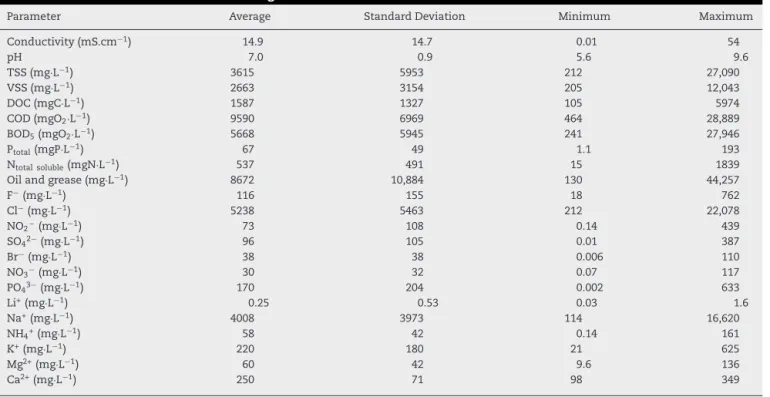
Table 3presents the mean (with respective standard devi-ation), the minimum and the maximum values obtained from the characterization of all samples. Again, the high BOD5and COD values show effluent’s strong contamination with organic matter. As was aforementioned, the wastewater also presents high values of TSS, O&G and salt content (analyzed in terms of Cl−and Na+concentrations and conductivity values). Typically the pH of fish processing industry wastewaters varies between 5.7 and 7.4, being on average equal to 6.4 (Technical Report Series, 1994). In this case, the effluent pH ranged between 5.6 and 9.6, with an average value of 7.0, similar to the value reported in the literature. TSS are one of the contaminants causing more impact on the environment. Its concentration on effluents of this type is generally high, between 2000 and 5000 mg/L) (Novatec, 1994; Prasertsan et al., 1994), which was also found in this study, with SST mean values of 3615 mg/L. The COD and BOD5 values ranged between 460–29,000 mg/L
and 240–28,000 mg/L, respectively, with both maximum val-ues registered at sample from 11/02/2014 collected in the morning. In the afternoon, for the same day, these concentra-tions were much lower, which confirms the high variability of this type of wastewaters. In the literature, the organic mat-ter content average values found in wastewamat-ters from fish processing industry are 1733 mg/L for BOD5and 3320 mg/L for COD (Prasertsan et al., 1994), values within the range found in this study. Comparing the values in terms of the relationship between the COD and BOD5, the value obtained in the liter-ature shows that the percentage of biodegradability (52%) is very close to the one found in this work (59%). The O&G show an average value of 8700 mg/L, very different from the one found by Prasertan et al. (1994) (3900 mg/L). This discrepancy is probably due to several factors that influence the pollutant load of this type of wastewaters. The average concentration of NaCl in the effluent is about 4600 mg/L. Although typical values of NaCl concentration on similar effluents were not referenced in the literature, this parameter is very important, since, when in high quantity it can be an inhibitor of biological processes.
3.2. Correlation analysis
270
Process Safety and Environmental Protection 1 0 2 ( 2 0 1 6 ) 263–276contribution of each parameter to the data set variance and the same weight, the normalization may amplify noise asso-ciated with minor variables that may have relatively larger analytical error.
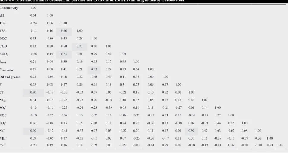
Table 4shows the correlation matrix achieved between all the 20 different fish canning wastewater samples after normalization. The negative correlation coefficients show a negative correlation whilst the positive correlation coefficients show a positive correlation between the two vari-ables. The closer this coefficient is to 1 the more similar the two variables are. If this coefficient is close to 0, it means that there is a very weak or perhaps even no relation between the two variables. It was considered the correlation coefficient value of 0.7 as the minimum acceptable threshold in order to exist a minimum statistical significance between two vari-ables. This threshold is supported bypvalues (probability of obtaining an effect at least as extreme as the one in the sam-ple data, assuming the truth of the null hypothesis) lower or equal to 0.05, corresponding to a percentage of significance of 95% This way, values with correlation coefficients > 0.7 were highlighted inTable 4. The high positive correlation between VSS and TSS (r= 0.86) indicates a high amount of suspended organic particles in the effluent in detriment to the mineral particles, showing also that when one increases the other increases too. The significant correlation between COD and VSS (r= 0.73) emphasizes the high proportion of particulate organic matter in the effluent. The BOD5 parameter is also considerably correlated with TSS (r= 0.73) which shows that a large portion of the particulate organic matter in the effluent is biodegradable. The high correlation observed between total soluble nitrogen and DOC (r= 0.83) refers to the fish organic nitrogen compounds. As expected, chloride and sodium ions show a high correlation with the conductivity (r= 0.9), since they are the ions with highest concentrations in the effluent. Finally, the correlation of 0.99 observed between sodium and chloride ions confirms that the most abundant salt in the efflu-ent is the sodium chloride from the brine step and from the seawater coming into the process.
As the results showed very few correlations near to−1 and +1, the information needed to describe the characterization of wastewater cannot be immediately reduced. Further elu-cidation may be obtained using more powerful chemometric techniques, such as CA and PCA, to group variables with sim-ilar variation pattern.
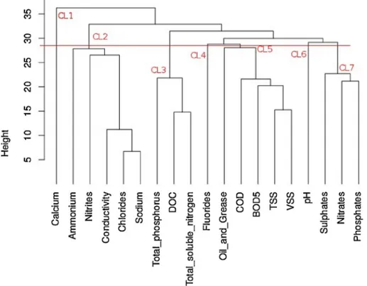
3.3. Cluster analysis
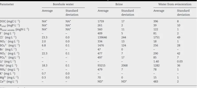
Cluster analysis is the most widely used unsupervised pat-tern recognition technique in chemometrics. This technique involves trying to determine relationships between samples without using prior information about these relationships. The raw data for cluster analysis consist of a number of objects and related measurements (Brereton, 1990). Objects or, in this case, physico-chemical parameters (pollution sources) were grouped in clusters in terms of their nearness or similarity. The resulting dendrogram can be observed inFig. 2, where 7 groups from the 19 analyzed parameters were obtained from cluster analysis. The first cluster (CL1) corresponds only to the calcium parameter. This result shows that calcium, as was also observed by the correlation analysis, does not correlate with any other parameter. To better understand its source, samples from borehole water, from brine water and, finally, from water from the eviscerating step were ana-lyzed regarding some important parameters. These results are present inTable 5. As it is possible to observe, the calcium only appears in the water from the eviscerating step and, despite not having been detected, probably in the brine water, since it was necessary to perform a very high dilution in order to analyze the ions in this effluent. In fact, calcium is present in small quantities in the global wastewater and, probably due to that, it appears as a cluster alone. The second cluster (CL2) has two sub-clusters: one corresponding to the ammo-nium parameter and a second one that includes the nitrites and, much closer, the conductivity, chlorides and sodium parameters. It has to be noted that the height in the dendro-gram represents accurately the linkage distance between the
Process
Safety
and
Environmental
Protection
1
0
2
(2016)
263–276
271
Table 4 – Correlation matrix between all parameters to characterize fish canning industry wastewaters.
Conductivity 1.00
pH 0.04 1.00
TSS -0.24 0.06 1.00
VSS -0.11 0.16 0.86 1.00
DOC 0.13 -0.08 0.45 0.28 1.00
COD 0.13 0.20 0.60 0.73 0.10 1.00
BOD5 -0.26 0.14 0.73 0.51 0.29 0.50 1.00
Ptotal 0.21 0.04 0.30 0.19 0.63 0.17 0.45 1.00
Ntotal soluble 0.17 0.08 0.41 0.21 0.83 0.24 0.29 0.64 1.00
Oil and grease 0.23 -0.08 0.18 0.32 -0.08 0.49 0.11 0.35 0.09 1.00
F- 0.08 0.03 0.27 0.26 0.01 0.18 0.31 0.25 0.09 0.17 1.00
Cl- 0.90 -0.17 -0.37 -0.33 0.07 0.05 -0.21 0.18 0.10 0.22 0.02 1.00
NO2- 0.34 0.07 -0.26 -0.25 0.20 -0.08 -0.01 0.35 0.08 0.07 0.13 0.42 1.00
SO42- -0.13 -0.16 -0.23 -0.24 0.23 -0.39 0.05 0.16 0.11 -0.21 -0.27 0.01 0.14 1.00
NO3- -0.10 -0.26 -0.08 0.10 -0.27 0.10 -0.08 -0.22 -0.41 0.03 0.10 -0.04 -0.25 0.22 1.00
PO43- 0.06 -0.04 0.03 0.15 -0.08 0.11 0.24 0.28 -0.06 0.13 -0.18 0.07 -0.09 0.44 0.32 1.00
Na+ 0.90 -0.12 -0.41 -0.37 0.07 0.03 -0.22 0.20 0.11 0.17 0.01 0.99 0.42 0.03 -0.02 0.08 1.00
NH4+ 0.29 -0.06 0.07 -0.05 -0.11 0.02 0.07 -0.25 -0.26 -0.17 0.11 0.30 0.16 -0.39 -0.15 -0.07 0.26 1.00
272
Process Safety and Environmental Protection 1 0 2 ( 2 0 1 6 ) 263–276Table 5 – Borehole water and water from brine and evisceration steps characteristics.
Parameter Borehole water Brine Water from evisceration
Average Standard deviation
Average Standard deviation
Average Standard deviation
DOC (mgC·L−1) NA* NA* 1759 17 396 8
Ptotal(mgP·L−1) NA* NA* 261 2 39 10
Ntotal soluble(mgN·L−1) NA* NA* 560 11 122 1
F−(mg·L−1) – – 409 5 81 2
Cl−(mg·L−1) 23.3 0.0 139646 244 1751 49
NO2−(mg·L−1) 2.0 0.0 334 13 18 1
SO42−(mg·L−1) 6.8 0.1 1476 124 256 28
Br−(mg·L−1) – – 47 0 – –
NO3−(mg·L−1) 22.3 0.1 477 7 290 42
PO43−(mg·L−1) – – 497 17 85 7
Li+(mg·L−1) – – – – 1.40 0.03
Na+(mg·L−1) 18.3 0.1 93215 2068 1282 36
NH4+(mg·L−1) – – 479 7 78 1
K+(mg·L−1) 0.7 0.0 – – – –
Mg2+(mg·L−1) 0.3 0.0 70 0 15 1
Ca2+(mg·L−1) – – ND* ND* 483 2
* NA: not analyzed.
* ND: not detected at dilution made.
original objects. The higher the correlation between parame-ters, the closer to the base (height = 0) of the dendrogram they
will be (Hand et al., 2001). So, this cluster (CL2) emphasizes the
close correlation between the sodium and chlorides and both with conductivity. However, these parameters also have some correlation with the nitrites and ammonium ions. By analyz-ing the entire cluster it is possible to verify that it is connected to the brine water. InTable 5it can be seen the high content of sodium and chloride ions in brine water and, consequently, its high conductivity values, which is in accordance withLefebvre and Moletta (2006). Despite presenting a lower correlation, it is also possible to observe that this water also contains nitrites and ammonium. These parameters could probably come from the oxidation after hydrolysis of the nitrogen present in the fish. Since the brine waters are kept for some time (they are normally discarded every two days), an oxidation process can occur, i.e., the hydrolysis of organic compounds, where organic nitrogen compounds are converted to ammoniacal nitrogen. If there is enough oxygen, there may still occur the ammo-niacal nitrogen oxidation to nitrites. According toSunny and Mathai (2013), wastewater streams with high blood content could present high ammonia concentration, which is the case of the brine water (Fig. 1). This way, this cluster points out that these parameters have the same source of pollution, i.e., it reflects the contribution of the brine water and its ions to the final effluent. The third cluster (CL3) groups total phosphorus, DOC and total soluble nitrogen parameters, showing that both nitrogen and phosphorus are present in the composition of fish particulate soluble organic matter. The results presented inTable 5, show that all these 3 parameters are presented in the brine water and in the water from evisceration, being the blood and the fish remains probably the contamination sources. The next cluster (CL4) is associated with fluorides. This cluster has a very high height, meaning that practically it has no correlation with any other parameter. In fact, this parameter appears in brine and evisceration waters (Table 5), showing that, in some way, it is associated with any fish com-pound. However, in the final effluent, with the presence of all other effluent streams, its concentration is low and practically invariable (Tables 1 and 2). The cluster number 5 (CL5) includes the oil and grease parameter and, with lower distance (higher
correlation), COD, BOD5, TSS and VSS parameters, i.e., it is probably connected with contaminations by particulate mat-ter and organics. Despite the oil and grease paramemat-ter showed lower correlation (higher height) with the other parameters, it also contributes to the organic particulate load of the efflu-ent (Sunny and Mathai, 2013) and is generally believed to be biodegradable (Chipasa and Medrzycka, 2006). The close correlation between TSS and VSS indicates, as already men-tioned, the high amount of suspended organic particles in the effluent. The connection of BOD5 and COD with those two parameters comes from the fact that both were analyzed without sample filtration, being also related to the particulate biodegradable organic matter of the effluent. These observa-tions lead to say that these parameters have the same source of organic pollution, probably associated with evisceration and cooking waters, which is in agreement with the pollution sources observed byCanales and Vidal (2002). The dendro-gram presents further 2 clusters, CL6 with pH parameter only and CL7 which includes the sulphates, the nitrates and the phosphates parameters. As it is possible to confirm by the cor-relation matrix (Table 4) the pH effectively does not correlate with any other parameter, making perfect sense to appear in a cluster alone. The correlations between sulphates, nitrates and phosphates showed that these compounds have the same contamination source, which may be the waters from factory cleaning and disinfection. The detergents used in this food industry are practically based on sulphates and phosphates, which confirms their correlation and the pollution source. The nitrates, although in lower concentration, also have some cor-relation with those parameters due to the high amount of borehole water used in the washing and cleaning steps, that has a significant concentration of nitrates (Table 5) and proba-bly also due to the mixture of these waters and the ones from the fish evisceration step (Mudge, 2007).
Process
Safety
and
Environmental
Protection
1
0
2
(2016)
263–276
273
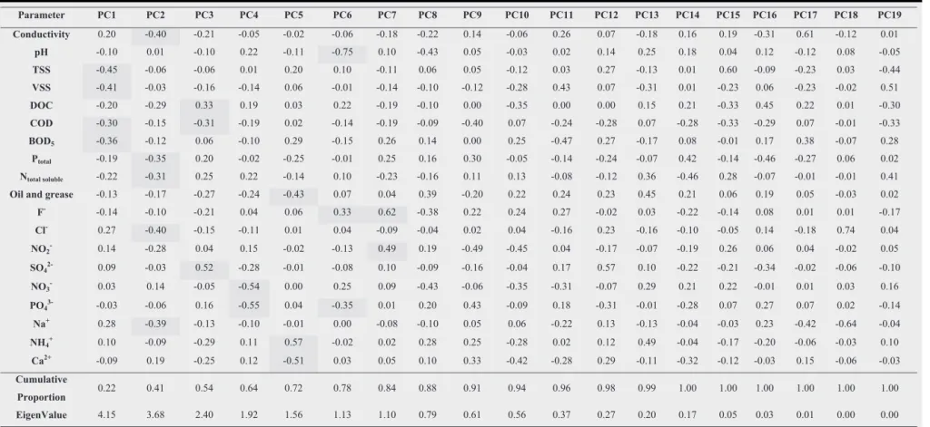
Table 6 – Principal components of PCA application for fish canning wastewater characteristics.
Parameter PC1 PC2 PC3 PC4 PC5 PC6 PC7 PC8 PC9 PC10 PC11 PC12 PC13 PC14 PC15 PC16 PC17 PC18 PC19
Conductivity 0.20 -0.40 -0.21 -0.05 -0.02 -0.06 -0.18 -0.22 0.14 -0.06 0.26 0.07 -0.18 0.16 0.19 -0.31 0.61 -0.12 0.01
pH -0.10 0.01 -0.10 0.22 -0.11 -0.75 0.10 -0.43 0.05 -0.03 0.02 0.14 0.25 0.18 0.04 0.12 -0.12 0.08 -0.05
TSS -0.45 -0.06 -0.06 0.01 0.20 0.10 -0.11 0.06 0.05 -0.12 0.03 0.27 -0.13 0.01 0.60 -0.09 -0.23 0.03 -0.44
VSS -0.41 -0.03 -0.16 -0.14 0.06 -0.01 -0.14 -0.10 -0.12 -0.28 0.43 0.07 -0.31 0.01 -0.23 0.06 -0.23 -0.02 0.51
DOC -0.20 -0.29 0.33 0.19 0.03 0.22 -0.19 -0.10 0.00 -0.35 0.00 0.00 0.15 0.21 -0.33 0.45 0.22 0.01 -0.30
COD -0.30 -0.15 -0.31 -0.19 0.02 -0.14 -0.19 -0.09 -0.40 0.07 -0.24 -0.28 0.07 -0.28 -0.33 -0.29 0.07 -0.01 -0.33
BOD5 -0.36 -0.12 0.06 -0.10 0.29 -0.15 0.26 0.14 0.00 0.25 -0.47 0.27 -0.17 0.08 -0.01 0.17 0.38 -0.07 0.28
Ptotal -0.19 -0.35 0.20 -0.02 -0.25 -0.01 0.25 0.16 0.30 -0.05 -0.14 -0.24 -0.07 0.42 -0.14 -0.46 -0.27 0.06 0.02
Ntotal soluble -0.22 -0.31 0.25 0.22 -0.14 0.10 -0.23 -0.16 0.11 0.13 -0.08 -0.12 0.36 -0.46 0.28 -0.07 -0.01 -0.01 0.41
Oil and grease -0.13 -0.17 -0.27 -0.24 -0.43 0.07 0.04 0.39 -0.20 0.22 0.24 0.23 0.45 0.21 0.06 0.19 0.05 -0.03 0.02
F- -0.14 -0.10 -0.21 0.04 0.06 0.33 0.62 -0.38 0.22 0.24 0.27 -0.02 0.03 -0.22 -0.14 0.08 0.01 0.01 -0.17
Cl- 0.27 -0.40 -0.15 -0.11 0.01 0.04 -0.09 -0.04 0.02 0.04 -0.16 0.23 -0.16 -0.10 -0.05 0.14 -0.18 0.74 0.04
NO2- 0.14 -0.28 0.04 0.15 -0.02 -0.13 0.49 0.19 -0.49 -0.45 0.04 -0.17 -0.07 -0.19 0.26 0.06 0.04 -0.02 0.05
SO42- 0.09 -0.03 0.52 -0.28 -0.01 -0.08 0.10 -0.09 -0.16 -0.04 0.17 0.57 0.10 -0.22 -0.21 -0.34 -0.02 -0.06 -0.10
NO3- 0.03 0.14 -0.05 -0.54 0.00 0.25 0.09 -0.43 -0.06 -0.35 -0.31 -0.07 0.29 0.21 0.22 -0.01 0.01 0.03 0.16
PO43- -0.03 -0.06 0.16 -0.55 0.04 -0.35 0.01 0.20 0.43 -0.09 0.18 -0.31 -0.01 -0.28 0.07 0.27 0.07 0.02 -0.14
Na+ 0.28 -0.39 -0.13 -0.10 -0.01 0.00 -0.08 -0.10 0.05 0.06 -0.22 0.13 -0.13 -0.04 -0.03 0.23 -0.42 -0.64 -0.04
NH4+ 0.10 -0.09 -0.29 0.11 0.57 -0.02 0.02 0.28 0.25 -0.28 0.02 0.12 0.49 -0.04 -0.17 -0.20 -0.06 -0.03 0.10
Ca2+ -0.09 0.19 -0.25 0.12 -0.51 0.03 0.05 0.10 0.33 -0.42 -0.28 0.29 -0.11 -0.32 -0.12 -0.03 0.15 -0.06 -0.03
Cumulative
Proportion 0.22 0.41 0.54 0.64 0.72 0.78 0.84 0.88 0.91 0.94 0.96 0.98 0.99 1.00 1.00 1.00 1.00 1.00 1.00
EigenValue 4.15 3.68 2.40 1.92 1.56 1.13 1.10 0.79 0.61 0.56 0.37 0.27 0.20 0.17 0.05 0.03 0.01 0.00 0.00
274
Process Safety and Environmental Protection 1 0 2 ( 2 0 1 6 ) 263–276Fig. 3 – Scree plot of variance vs principal components.
suggested by the cluster analysis represented by the dendro-gram inFig. 2, it would be advantageous to somehow reduce the number of variables in this data set for future monitoring of wastewater quality, obtaining likewise a correct wastewater characterization, with minimal associated costs. So, as 7 main clusters were found and since, in principle, they are associated to the main characteristics of this type of effluents, to obtain a correct, but faster and cheaper characterization of fish canning industry wastewaters, to be possible to forward it for the most adequate treatment process, it is necessary to analyze only 7 main parameters (rather than the 19 original parameters).
3.4. Principal component analysis
In order to support the cluster analysis classification, princi-pal component analysis was applied to the whole set of data. PCA was applied as a non-parametric method of classification, in order to classify the analyzed parameters into classes (PCs) having the same pollution behavior and differing from those in other classes, enabling the reduction of the dimensionality of the data set and the costs associated. The PCs, the eigen-values and the cumulative proportion of variance explained by each PC are shown inTable 6. Although the number of PCs equals the number of analyzed parameters, generally, most of the variance in the data is explained by the first few PCs that can be used to represent the original parameters ( Abdul-Wahab et al., 2005). So, the first step in PCA is to select the number of PCs to retain. As was mentioned in the Materials and Methods section, there are three main criteria to deter-mine how many PCs to keep. Among these criteria, criterion 3 is in fact a useful visual aid, a scree plot, where variances are ordered from largest to smallest, being a good starting point to decide how many PCs to retain. On this plot, there is usually an “elbow” below which all variances are small, leading to retain only the PCs above it (Mudge, 2007). The scree plot for this study is shown inFig. 3. Through its inspection it is possible to observe an elbow at the seventh PC. Thus, from the infor-mation on the scree plot and from criterion 2, that defends that the principal components to retain are the ones whose eigenvalues are higher than 1 (Kaiser criterion), 7 principal components were retained. In fact, in this case, the fulfillment of these two criteria automatically leads to fulfillment of crite-rion 1 since, as can be seen on Table 7, the first seven principal
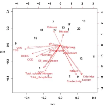
Fig. 4 – Biplot (PC1 vs PC2) for fish canning industry wastewaters parameters.
components describe 84% of total variance (>70%), i.e., explain 84% of the relevant information from the data. It is also possi-ble to verify that the first component represents the maximum variation of the data set, accounting for 22% of total vari-ance. However, the proportion of total variance that describes adequately a data set varies with the field of application. In some cases it might be sufficient the first few components to describe a significant proportion of variance, but in other cases many more PCs could be necessary (Hand et al., 2001). The relatively high number of PCs needed to explain the whole variability of fish canning industry wastewater characteristics has to do with the fact that the environmental datasets used are very influenced by a high number of variability sources, as was confirmed.
Process Safety and Environmental Protection 1 0 2 ( 2 0 1 6 ) 263–276
275
comes to emphasize the effluent contamination by cleaning waters, with high contributions of NO3− and PO43− (−0.54 and−0.55, respectively) and also with a moderate contribu-tion of SO42− (−0.28). This PC could be associated with CL7 observed in the cluster analysis. PC5 is associated essentially with parameters that present almost no correlation with other ones, namely Ca2+, NH
4+and O&G. The weak correlations can be confirmed by their respective height in the dendrogram (Fig. 2). PC6 is heavily loaded by pH and F-, which also presents almost no correlation with other parameters. It has also a con-tribution of PO43-, despite of being lower than its contribution to PC4. Finally, PC7 includes F−and NO
2-, parameters that were already included in other PCs, showing that probably only 6 PCs are sufficient to describe the data set. Effectively, these six first PCs already describe almost 80% of the total variance (Table 6). Moreover, the large number of parameters associated in PC1 and PC2 emphasizes the importance of those parame-ters and the idea of reducing the analyzed wastewater quality parameters.
As mentioned, it is possible to notice that the PCA results do not identify exactly the same grouping as the cluster analysis. This is probably due to the fact that the PCA explains only part of the variance among samples, and it is not guaranteed that the sacrificed information is not relevant to the wastewater characterization. So, both statistical methods should be used to explain the data. The results from PCA and cluster anal-ysis could be also compared with the information obtained by plotting the first two PCs (PCs with the large number of parameters), leading to more accurate conclusions. Therefore,
Fig. 4shows the plot of PC1 against PC2, where it is possible to observe the variables behavior and the identification numbers for each collected sample. It is clear from this diagram that there are parameters very different from the others, where ones lie in the right corner and the other ones in the left. When a parameter is located at a certain distance from the other parameters, it means that it differs significantly from the other ones, even if only for one sample. When two parameters are together on the same side of the biplot it means that they are in the same cluster (Gabriel, 1971). As can be seen inFig. 4, there are essentially 3 well defined groups, which coincides with the previously defined classes: one composed by con-ductivity, Na+, Cl−and NO
2-, another composed by DOC, Ntotal solubleand Ptotaland a third one composed by TSS, VSS, BOD5 and COD. The rest of the parameters appear more dispersed into the components space, displaying a more individualized behavior. These results show that the main sources of con-tamination of this type of effluents are the brine waters and the waters from the evisceration step.
The results obtained with all the used statistical method-ologies led, this way, to identify the main fish canning industry wastewaters pollution sources, allowing also the creation of groups of quality parameters and defining which and how many parameters are necessary to characterize with maximum precision the fish canning industry wastewaters, avoiding, at the same time, redundant measurements. Thus, it was concluded that only 7 of the 19 studied parameters should be selected. The selection of the parameters (from each cluster found) to analyze in a future wastewater quality mon-itoring process depends on several factors: the easiness of the analysis, the necessary labor, the lab availabilities, con-sumables and energy costs, the equipment costs, the waste produced in the analysis, the risks for the operator, etc. In this work, the 7 parameters more suitable to correctly ana-lyze the fish canning wastewater, allowing an easier and faster
characterization, with lower costs are: from CL1, CL4 and CL6, the Ca2+, F−and pH parameters, respectively, i.e., the param-eters that are in a cluster alone; from CL2 the conductivity, which is the parameter that is easier to analyze and presents minor costs, since it avoids the use of an ionic chromatograph; from CL3 the selected parameter is the DOC since it is analyzed by a simpler method than the Ptotaland it does not require an extra module in the Total Organic Carbon analyzer as the Ntotal
soluble; from CL5 the simplest and cheapest parameter to ana-lyze is the TSS, since it does not involve any digestion, is not time consuming and spends little energy; finally, from CL7 the choice of the parameter to be analyzed is indifferent, as all three parameters are analyzed in the same way.
4.
Conclusions
In order to evaluate the main wastewater pollution sources of fish canning industry wastewaters and to reduce the param-eters to analyze wastewater characterization, multivariate statistical methods were applied to twenty wastewater sam-ples collected during eight months (from November 2013 to June 2014).
The results achieved demonstrate that correlation anal-ysis, CA and PCA are powerful tools to find relationships among many variables and to group samples in large datasets. Correlation analysis allowed to interpret the linear correla-tions between all the parameters in study, the cluster analysis led to group the 19 parameters in only 7 clusters, show-ing the similarity of the parameters between each cluster and their relations with the pollution sources, finally, PCA allowed the reduction of 19 PCs to only 6, that explained 78% of the total variance of the original data set. The wastewa-ter pollution sources were identified based on the created groups of wastewater quality parameters, recognizing the brine waters and the waters from the eviscerating step as the main sources of the pollution. The 7 sufficient important parameters to achieve a fully characterization of fish canning industry wastewaters proved to be the DOC, the TSS, the con-ductivity, the pH, the Ca2+, F− and one of the parameters SO42-, NO3−and PO43concentrations. Therefore, this evalu-ation served as an excellent tool to establish guidelines for a monitoring program of fish canning wastewaters quality and the improvement of their treatment process, avoiding redun-dant measurements and allowing to minimize, at the same time, the associated costs. In fact, the methodology presented in this study is quite important since it can be applied in differ-ent industrial plants that generate effludiffer-ents with very variable composition over time and want (or need to comply with legal requirements) to install a treatment system (WWTP).
Acknowledgments
This work is partially supported by project PEst-C/EQB/LA0020/2013, financed by FEDER through COMPETE –
Programa Operacional Factores de Competitividade and by FCT
– Fundac¸ão para a Ciência e a Tecnologiaand by ValorPeixe –
276
Process Safety and Environmental Protection 1 0 2 ( 2 0 1 6 ) 263–276References
Abdul-Wahab, S.A., Bakheit, C.S., Al-Alawi, S.M., 2005. Principal component and multiple regression analysis in modelling of ground-level ozone and factors affecting its concentrations. Environ. Modell. Soft. 20, 1263–1271.
Anderson, T.W., 1996. R. A. Fisher and multivariate analysis. Stat. Sci. 11, 20–34.
APHA, 2005. Standard Methods for the Examination of Water and Wastewater, 21st ed, Washington, DC, USA.
Babu, S.C., Gajanan, S.N., Sanyal, P., 2014. Chapter 8 – Indicators and Causal Factors of Nutrition — Application of Correlation Analysis. Food Security, Poverty and Nutrition Policy Analysis (Second Edition) – Statistical Methods and
Applications.
Boruvka, L., Vacek, O., Jehlicka, J., 2005. Principal component analysis as a tool to indicate the origin of potentially toxic elements in soils. Geoderma 128, 289–300.
Brereton, R.G., 1990. Chemometrics – Applications of Mathematics and Statistics to Laboratory Systems. Ellis Horwood Limited, West Sussex, UK.
Canales, C., Vidal, A., 2002. Guía De Mejores Técnicas Disponibles En Espa ˜na Del Sector De Productos Del Mar. Ministerio De Medio Ambiente. Ministerio De Agricultura, Pesca Y Alimentación.
Cattell, R.B., 1966. The scree test for the number of factors. Multivar. Behav. Res. 1, 245–276.
Chipasa, K.B., Medrzycka, K., 2006. Behavior of lipids in biological wastewater treatment processes. J. Ind. Microbiol. Biotechnol. 33, 635–645.
Chowdhury, P., Viraraghavan, T., Srinivasan, A., 2010. Biological treatment processes for fish processing wastewater – a review. Bioresour. Technol. 101, 439–449.
Cristóvão, R.O., Botelho, C.M., Martins, R.J.E., Loureiro, J.M., Boaventura, R.A.R., 2015. Fish canning industry wastewater treatment for water reuse – a case study. J. Clean. Prod. 87, 603–612.
Cristóvão, R.O., Botelho, C.M., Martins, R.J.E., Loureiro, J.M., Boaventura, R.A.R., 2014. Primary treatment optimization of a fish canning wastewater from a Portuguese plant. Water Res. Ind. 6, 51–63.
Cristóvão, R.O., Botelho, C.M.S., Martins, R.J.E., Boaventura, R.A.R., 2012. Chemical and biological treatment of fish canning wastewaters. Int. J. Biosci. Biochem. Bioinf. 2, 237.
Delgado, C.L., Wada, N., Rosegrant, M.W., Meijer, S., Ahmed, M., 2003. The Future of Fish: Issue and Trend to 2020 (Issue Brief). International Food Policy Research Institute (Washington, DC)/World Fish Center (Penang, Malaysia).
Gabriel, K.R., 1971. The biplot graphic display of matrices with application to principal component analysis. Biometrika 58, 453–467.
Gharsallah, N., Khannous, L., Souissi, N., Nasri, M., 2002. Biological treatment of saline wastewaters from marine – products processing factories by a fixed-bed reactor. J. Chem. Technol. Biotechnol. 77, 865–870.
Hand, D., Mannila, H., Smyth, P., 2001. Principles of Data Mining. The MIT Press, Cambridge, Massachussets, England.
Hatcher, L., Stepansku, E., 1994. A Step by Step Approach to Using the SAS System for Univariate and Multivariate Statistics. SAS Institute, Inc., Cary, NC.
Jackson, J., 2002. Data mining: a conceptual overview. Commun. Assoc. Inform. Syst. 8, 267–296.
Kaiser, H.F., 1960. The application of electronic computers to factor analysis. Educ. Psychol. Meas. 20, 141–151.
Kara, D., 2009. Evaluation of trace metal concentrations in some herbs and herbal teas by principal component analysis. Food Chem. 114, 347–354.
Lee, M.W., Hong, S.H., Choi, H., Kim, J.-H., Lee, D.S., Park, J.M., 2008. Real-time remote monitoring of small-scaled biological wastewater treatment plants by a multivariate statistical
process control and neural network-based software sensors. Process Biochem. 43, 1107–1113.
Lefebvre, O., Moletta, R., 2006. Treatment of organic pollution in industrial saline wastewater: a literature review. Water Res. 40, 3671–3682.
Magyar, N., Hatvani, I.G., Székely, I.K., Herzig, A., Dinka, M., Kovács, J., 2013. Application of multivariate statistical methods in determining spatial changes in water quality in the Austrian part of Neusiedler See. Ecol. Eng. 55, 82–92. Mudge, S.M., 2007. Multivariate statistical methods in
environmental forensics. Environm. Forensics 8, 155–163. NovaTec Consultants Inc, EVS Environmental Consultants, 1994.
Wastewater Characterization of Fish Processing Plant Effluents – A Report to Water Quality/Waste Management Committee, Fraser River Estuary Management Program, Waste Manag.
Ouali, A., Azri, C., Medhioub, K., Ghrabi, A., 2009. Descriptive and multivariable analysis of the physico-chemical and biological parameters of Sfax wastewater treatment plant. Desalination 246, 496–505.
Paoletti, I., De Berardis, B., Diociaiuti, M., 2002. Physico-chemical characterization of the inhalable particulate matter (PM10) in an urban area: an analysis of the seasonal trend. Sci. Total Environ. 292, 265–275.
Pires, J.C.M., Martins, F.G., Sousa, S.I.V., Alvim-Ferraz, M.C.M., Pereira, M.C., 2008. Selection and validation of parameters inmultiple linear and principal component regressions. Environ. Modell. Soft. 23, 50–55.
Prasertsan, P., Jung, S., Buckle, K.A., 1994. Anaerobic filter treatment of fishery wastewater. World J. Microbiol. Biotechnol. 10, 11–13.
Singh, K.P., Malik, A., Sinha, S., 2005. Water quality assessment and apportionment of pollution sources of Gomti river (India) using multivariate statistical techniques – a case study. Anal. Chim. Acta 538, 355–374.
Soares, J.O., Marquês, M.M.L., Monteiro, C.M.F., 2003. A multivariate methodology to uncover regional disparities: a contribution to improve European Union and governmental decisions. Eur. J. Oper. Res. 145, 121–135.
Song, Y., Xie, S.D., Zhang, Y.H., Zeng, L.M., Salmon, L.G., Zheng, M., 2006. Source apportionment of PM2.5 in Beijing using principal component analysis/absolute principal component scores and UNMIX. Sci. Total Environ. 372, 278–286.
Sunny, N., Mathai, L., 2013. Physicochemical process for fish processing wastewater. Int. J. Innov. Res. Sci. Eng. Technol. 2, 901–905.
Technical Report Series FREMP WQWM-93-10, DOE FRAP 1993-39, 1994. Wastewater Characterization of Fish Processing Plant Effluents. Fraser River Estuary Management Program, New West Minister, BC.
Viana, M., Querol, X., Alastuey, A., Gil, J.I., Menéndez, M., 2006. Identification of PM sources by principal component analysis (PCA) coupled with wind direction data. Chemosphere 65, 2411–2418.
Wan, J., Huang, M., Ma, Y., Guo, W., Wang, Y., Zhan, H., Li, W., Sun, X., 2011. Prediction of effluent quality of a paper mill
wastewater treatment using an adaptive network-based fuzzy inference system. Appl. Soft. Comput. 11, 3238–3246.
Wang, Y., Wang, P., Bai, Y., Tian, Z., Li, J., Shao, X., Mustavich, L.F., Li, B.-L., 2013. Assessment of surface water quality via multivariate statistical techniques: a case study of the Songhua River Harbin region. China J. Hydro-environ. Res. 7, 30–40.
Yoo, C.K., Vanrolleghem, P.A., Lee, I.-B., 2003. Nonlinear modeling and adaptive monitoring with fuzzy and multivariate statistical methods in biological wastewater treatment plants. J. Biotechnol. 105, 135–163.