Lisbon, Portugal, July 24-27, 2018
FIRST-ORDER GBT FOR THIN-WALLED MEMBERS WITH
ARBITRARY CROSS-SECTION AND CIRCULAR AXIS
Nuno R. S. Peres*, Rodrigo M. Gonçalves* and Dinar Camotim**
* CERIS, ICIST and Departamento de Engenharia Civil, Faculdade de Ciências e Tecnologia, Universidade NOVA de Lisboa, 2829-516 Caparica, Portugal
e-mails: [email protected], [email protected]
** CERIS, ICIST, DECivil, Instituto Superior Técnico, Universidade de Lisboa, 1049-001 Lisbon, Portugal e-mail: [email protected]
Keywords: Thin-walled members; Generalised Beam Theory (GBT); Naturally curved bars with circular axis; Cross-section deformation.
Abstract. This work assesses the first-order behavior of thin-walled bars with deformable cross-section and circular axis, without pre-twist, with the help of the Generalised Beam Theory (GBT) formulation previously developed by the authors (which dealt only with simple cross-sections without distortional deformation). Moreover, this paper presents a novel and systematic procedure to obtain the deformation modes for arbitrary flat-walled cross-sections (open, closed or “mixed”). The standard GBT kinematic assumptions, although much more complex than for the prismatic case, are employed to subdivide the modes in a meaningful way, maintaining the same nomenclature used for prismatic bars, and to reduce the number of DOFs necessary to achieve accurate results. It is also shown that the curvature of the bar has a significant influence on the deformation mode shapes. Finally, a standard displacement-based GBT finite element (FE) is employed to solve a set of representative examples, proving the efficiency of the proposed formulation and showing the peculiar behavior of curved bars. A comparison with shell FE models is also provided for validation purposes.
1 INTRODUCTION
Generalised Beam Theory (GBT) is a thin-walled bar theory that incorporates cross-section plane and out-of-plane deformation, through the consideration of hierarchical and structurally meaningful cross-section DOFs, the so-called “cross-section deformation modes”. GBT was initially proposed by Schardt [1, 2] and it is presently well-established as an efficient, versatile, accurate and insightful approach to asses the structural behavior of thin-walled prismatic bars (see, e.g., [3-5]).
Recently, the authors developed a first-order GBT formulation for thin-walled bars with circular axis, without pre-twist [6]. This formulation constitutes an extension of the prismatic case, still allowing for the incorporation (or not) of the usual GBT strain assumptions. Moreover, it extends the classic theories of Winkler [7] and Vlasov [8]. The proposed formulation can handle all types of deformation modes, but their systematic determination for complex cross-sections was not presented due to the fact that the so-called “natural Vlasov
according to specific kinematic constraints, ensuring that the modal decomposition of the solutions provides in-depth insight into the mechanics of the problem under consideration. A set of representative numerical examples is presented and solved using a standard displacement-based GBT finite element (FE), to show the capabilities of the proposed formulation.
The notation follows that introduced in [10, 13, 14]. The subscript commas indicate derivatives (e.g., 𝑓,𝑥 = 𝜕𝑓/𝜕𝑥), but the prime is reserved for a derivative with respect to the beam axis arc-length 𝑋, i.e., (⋅)′ = 𝜕(⋅)/𝜕𝑋. Finally, the superscripts (⋅)𝑀 and (⋅)𝐵 designate plate-like membrane and bending terms, respectively.
2 FIRST-ORDER GBT FOR MEMBERS WITH CIRCULAR AXIS
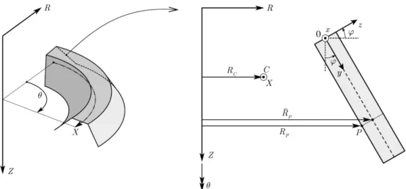
The formulation presented in [6] is briefly reviewed in this section for completeness of the paper. A curved thin-walled member is shown in Fig. 1, along with the global cylindrical (𝜃, 𝑍, 𝑅) and the local wall (𝑥, 𝑦, 𝑧) coordinate systems. The member axis arc-length coordinate 𝑋 lies on the 𝑍 = 𝑍𝐶 horizontal plane and has constant curvature equal to 1/𝑅𝐶, and defines the arbitrary cross-section “center” 𝐶. The wall local axes 𝑦 and 𝑧 define, respectively, the mid-line and through-thickness directions, and 𝑥 is concentric to 𝑋.
Figure 1: Global and local (wall) axes for a naturally curved thin-walled member.
The standard GBT variable separation technique is employed for the membrane displacement components (𝑢, 𝑣, 𝑤) along (𝑥, 𝑦, 𝑧), making it possible to write
𝑢𝑀 = 𝒖̅𝑇(𝑦)𝝓′(𝑋), 𝑣𝑀 = 𝒗̅𝑇(𝑦)𝝓(𝑋), 𝑤𝑀 = 𝒘̅𝑇(𝑦)𝝓(𝑋) (1)
where 𝒖̅, 𝒗̅, 𝒘̅ are column vectors collection the mid-line displacement components of the deformation modes functions and 𝝓 is a column vector containing their respective amplitude functions. Kirchhoff’s thin-plate assumption is employed to reduce the number of admissible deformation modes and eliminate plate-like shear locking, making it possible to write the displacements in terms of the membrane displacements, as
𝑼 = [𝑈𝑈xy
𝑈z
] = 𝚵𝑈[𝝓𝝓′] , 𝚵𝑈 = [
𝟎 𝒖̅𝑇+ 𝑧𝐾
𝑦𝛽̅𝒖̅𝑇− 𝑧𝛽̅𝒘̅𝑇
𝒗̅𝑇− 𝑧𝒘̅ ,𝑦
𝑇 𝟎
𝒘̅𝑇 𝟎
] , (2)
The strains are divided into membrane and bending components, being given by
𝜺 = 𝜺𝑀 + 𝜺𝐵 = 𝚵 𝜀[
𝝓 𝝓′
𝝓′′] , 𝚵𝜀 = 𝚵𝜀
𝑀+ 𝚵
𝜀
𝐵, 𝚵
𝜀(⋅)=
[ (𝝃11(⋅))
𝑇
𝟎 (𝝃13(⋅))𝑇 (𝝃21(⋅))𝑇 𝟎 𝟎
𝟎 (𝝃32(⋅))𝑇 𝟎 ]
, (3)
where 𝝃𝑖𝑗(⋅) are column vectors reading
𝝃11𝑀 = 𝛽̅(𝐾𝑦𝒘̅ − 𝐾𝑧𝒗̅), (4)
𝝃13𝑀 = 𝛽̅𝒖̅, (5)
𝝃21𝑀 = 𝒗̅,𝑦, (6)
𝝃32𝑀 = 𝛽̅𝒗̅ + 𝛽̅𝐾𝑧𝒖̅ + 𝒖̅,𝑦, (7)
𝝃11𝐵 = −𝑧𝛽̅(−𝐾𝑧𝒘̅,𝑦+ 𝛽̅𝐾𝑦2𝒘̅ − 𝛽̅𝐾𝑦𝐾𝑧𝒗̅), (8)
𝝃13𝐵 = −𝑧𝛽̅2𝒘̅, (9)
𝝃21𝐵 = −𝑧𝒘̅,𝑦𝑦, (10)
𝝃32𝐵 = −𝑧𝛽̅(2𝒘̅,𝑦+ 2𝛽̅𝐾𝑧𝒘̅ − 𝐾𝑦𝒖̅,𝑦+ 𝛽̅𝐾𝑦𝒗̅ − 𝛽̅𝐾𝑦𝐾𝑧𝒖̅). (11)
The stresses 𝝈 are obtained from the strains using the standard plane stress constitutive relation for elastic isotropic materials. If null membrane transverse extensions are assumed, the Poisson terms for the membrane strains must be eliminated and the membrane and bending terms may be uncoupled through the substitution 𝑅/𝑅𝐶 ≈ 𝑅̅/𝑅𝐶 = 1/𝛽̅.
The homogeneous form of the differential equilibrium equation reads
𝗖𝝓′′′′− (𝗗 − 𝗙 − 𝗙𝑇)𝝓′′+ (𝗚 + 𝗘 + 𝗘𝑇+ 𝗕)𝝓 = 𝟎, (12)
where 𝗗 = 𝗗𝟏− 𝗗𝟐− 𝗗𝟐𝑇, the GBT modal matrices are given by
𝗕 = ∫1−𝜈𝐸2
𝐴 𝑅
𝑅𝐶𝝃21𝝃21
𝑇 𝑑𝐴, 𝗖 = ∫ 𝐸 1−𝜈2
𝐴 𝑅
𝑅𝐶𝝃13𝝃13
𝑇 𝑑𝐴, (13a)
𝗗𝟏 = ∫𝐺𝑅𝑅𝐶
𝐴 𝝃32𝝃32
𝑇 𝑑𝐴, 𝗗
𝟐 = ∫1−𝜈𝜈𝐸2
𝐴 𝑅
𝑅𝐶𝝃21𝝃13
𝑇 𝑑𝐴, (13b)
𝗘 = ∫1−𝜈𝜈𝐸2
𝐴 𝑅
𝑅𝐶𝝃11𝝃21
𝑇 𝑑𝐴, 𝗙 = ∫ 𝐸 1−𝜈2
𝐴 𝑅
𝑅𝐶𝝃11𝝃13
𝑇 𝑑𝐴, (13c)
𝗚 = ∫1−𝜈𝐸2
𝐴 𝑅
𝑅𝐶𝝃11𝝃11
𝑇 𝑑𝐴, (13d)
3 DEFORMATION MODES
The proposed procedure to determine the cross-section deformation modes shares concepts with those presented in [10-12] for the prismatic case. The cross-section is first discretized using (i) “natural” nodes, automatically located at wall mid-line intersections and free edges, and (ii)
“intermediate” nodes, arbitrarily located in the walls, between the natural nodes, defining the
discretization level.
An initial basis for the deformation modes is generated, using three DOFs per node, namely two in-plane displacements (the in-plane rotation is condensed, as in the classic GBT formulations) and one warping displacement. Hermite cubic functions are employed between nodes for the 𝑤̅𝑘 displacements, and linear functions for 𝑣̅𝑘 and 𝑢̅𝑘. For members with circular axis, as shown in [6], the linear 𝑢̅𝑘 functions are consistent with the null membrane transverse extension and Vlasov assumptions, which read, from the strain-displacement equations,
𝑣̅𝑘,𝑦 = 0, 𝑣̅𝑘 = −𝑢̅𝛽̅𝑘,𝑦− 𝐾𝑧𝑢̅𝑘. (14)
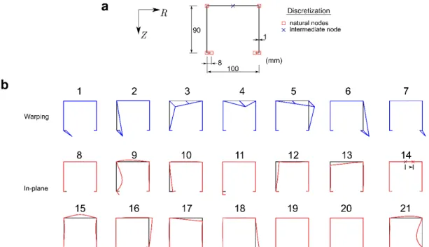
The first assumptions leads to 𝑣̅𝑘 being constant in each wall. The latter constraint is more complex than that concerning prismatic members, and shows that for 𝑣̅𝑘 to be constant, 𝑢̅𝑘 must be linear (at the most). For illustrative purposes, Fig. 2 shows the initial, or “elementary”, modes for a lipped channel discretized with a single intermediate node in the web, leading to 7 warping and 14 in-plane deformation modes, totaling 21 modes.
The final deformation modes are calculated from the initial basis through change of basis operations, using generalized eigenvalue problems involving the GBT modal matrices, and assuming 1/𝑅𝐶 ≈ 1/𝛽̅, leading to membrane-bending uncoupling. The following mode sets are defined:
• Vlasov natural modes, generated from the natural node warping DOFs and complying with the Vlasov and null membrane transverse extensions assumptions. As in the classic GBT, this set is subdivided into (i) distortional and (ii) rigid-body modes (extension, bending and, for open sections, torsion).
• Local-plate modes, also satisfying 𝛾𝑥𝑦𝑀 = 𝜀𝑦𝑦𝑀 = 0, but involving essentially plate bending, with minute warping.
• Shear modes, with 𝛾𝑥𝑦𝑀 ≠ 0 and 𝜀𝑦𝑦𝑀 = 0, which are subdivided into (i) cell shear cell flow modes (for closed sections only, including torsion), (ii) warping functions of the Vlasov modes and (iii) additional warping functions. The shear modes generated by the intermediate node DOFs are included in the latter subset.
• Transverse extension modes, with 𝜀𝑦𝑦𝑀 ≠ 0, including the intermediate node DOFs.
3.1 Procedure to calculate the deformation modes
The strain-displacement relations of Eqs. (3)-(11) show that (i) the Vlasov constraint can be enforced by calculating the nullspace of 𝗗𝟏𝑀 and (ii) the null membrane transverse extension modes belong to the nullspace of 𝗕𝑀. Both matrices are necessarily positive semi-definite in
the space defined by the “elementary” deformation modes, and one first solves
(𝗕𝑀− 𝜆𝑰)𝒗 = 𝟎, (15)
Figure 2: Lipped channel: (a) cross-section geometry and discretization, (b) initial deformation modes.
The 𝜆 = 0 eigenvectors satisfy the null membrane transverse extension assumption and thus contain the remaining mode sets. In this space, one solves
( 𝗗𝟏𝑀− 𝜆𝑰)𝒗 = 𝟎, (16)
where the 𝜆 = 0 eigenvectors define a basis for the Vlasov and local-plate modes. The procedure devised by Schardt [2] for the hierarchization of these modes for prismatic members is employed, namely by solving
(𝗕𝐵− 𝜆(𝗖𝑀+ 𝗖𝐵))𝒗 = 𝟎, (17)
with (i) the 𝜆 = 0 eigenvectors defining the rigid-body mode subspace and (ii) the 𝜆 ≠ 0 eigenvectors correspond to the Vlasov distortional and local-plate modes (see [10] for the computation of their number).
The rigid-body modes are obtained following the classic formulations for beams with circular axis (e.g., [15, 16]): 𝐶 coincides with the centroid and the kinematic description of the axis is expressed in terms of tangential (mode 1), radial (mode 2) and out-of-plane (mode 3) rigid-body displacements.
The torsion mode for open sections is, as usual, calculated by working in the 4-D rigid-body mode space and calculating the 𝜆 ≠ 0 eigenvector of
(𝗗𝟏𝐵− 𝜆𝗖𝑀)𝒗 = 𝟎, (18)
since the nullspace of 𝗗𝟏𝐵 corresponds to 𝛾𝑥𝑦𝐵 = 0 and the use of matrix 𝗖𝑀 enforces orthogonality of the torsion warping stress resultant with respect to the first three modes. As discussed next, for closed sections, the torsional mode belongs to the shear mode space.
The orthogonal complement, in the 𝗖𝑀 sense, of the II subset plus mode 1, in the warping mode space, must be obtained for subsequent calculation of the III modes. The modes are then orthogonalized and hierarchized through
(𝗗𝟏𝑀 − 𝜆𝗖𝑀)𝒗 = 𝟎. (19)
The calculation of the I modes is more involved. First, a basis pertaining to independent 𝑣̅𝑘 displacements of the walls is obtained and added to the II and III shear modes, excluding the warping functions of the bending modes (2 and 3). Then, one solves
(𝗕𝐵− 𝜆(𝗕𝐵+ 𝗗 𝟏
𝑀)) 𝒗 = 𝟎, (20)
where the eigenvectors associated with 0 < 𝜆 < 1 define the I shear subspace excluding torsion. The torsional mode is found in the nullspace of 𝗕𝐵, from the previous 𝜆 = 0 eigenvector set, by calculating the single non-null eigenvalue of
(𝗗𝟏𝐵− 𝜆𝗗𝟏𝑀)𝒗 = 𝟎. (21)
Following the same procedure as in [12], the shear modes I are placed between modes 3 and the first distortional Vlasov mode. The final deformation modes are normalized as follows: (i) the rigid-body modes correspond to unit displacements and/or rotations, (ii) the Vlasov, local-plate and I shear modes have a maximum unit in-plane displacement, (iii) the II and III shear modes have a maximum unit warping displacement and (iv) the transverse extension modes have a maximum unit membrane transverse extension.
The procedure was implemented in MATLAB [17]. Using an Intel Core i7-9700HQ [email protected] GHz processor, the runtime for an open cross-section with 20 modes is approximately 0.2 seconds, and for a closed cross-section with 50 modes, it increases to about 2 seconds.
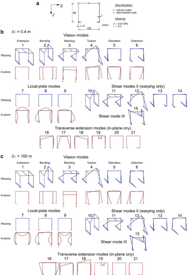
For illustrative purposes, Figs. 3 and 4 show the deformation modes for two cross-sections, namely a lipped channel (open section) and a three-cell cross-section (closed section), considering 𝑅𝐶 = 0.4 m and 𝑅𝐶 = 100 m (Fig. 4c shows only selected modes). In both cases, 𝐶 corresponds to the cross-section centroid. It is observed that the mode configurations change with 𝑅𝐶. In particular, the local and distortional modes (and their shear mode counterparts) lose their symmetry/anti-symmetry as this value decreases. Note that, for 𝑅𝐶 = 0.4 m, mode 1 does not correspond to uniform warping and mode 3 includes a torsional rotation. Moreover, in Fig. 4b, the center of rotation of mode 4 is slightly offset to the right of the centroid.
4 NUMERICAL EXAMPLES
discretization with 50 elements and 15 deformation modes. The results are compared with refined 4 node MITC shell finite element models, using ADINA [18].
4.1 Lipped channel beam subjected to two out-of-plane tip loads
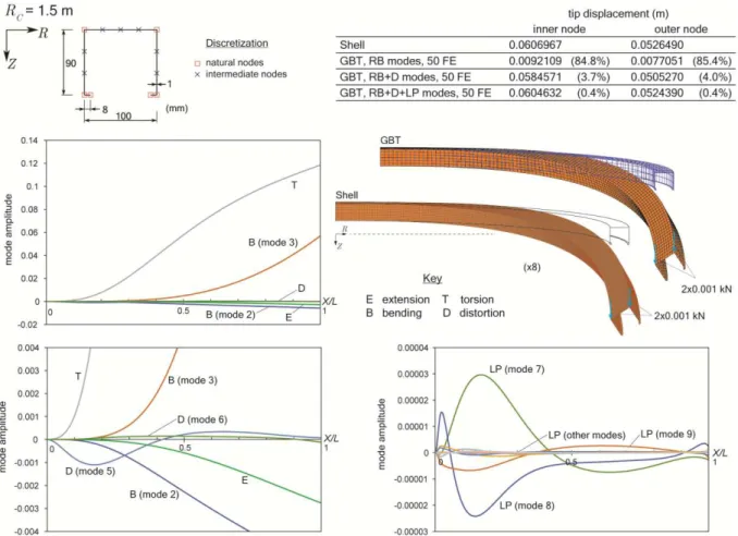
Fig. 5 shows a lipped channel section cantilever beam, whose cross-section dimensions and deformation modes are presented in Fig. 3 and is subjected to two out-of-plane tip loads. The GBT analysis was carried out with a cross-section discretization with 7 nodes, as shown in Fig. 5.
Figure 5: Lipped channel 90º cantilever beam subjected to two out-of-plane tip loads.
The table in Fig. 5 shows the tip vertical displacements obtained with a refined shell finite element model and GBT, the latter using 50 finite elements and different combinations of the following mode sets: (i) rigid-body (RB), (ii) Vlasov distortional (D) and (iii) local-plate modes (LP). The shear (S) and transverse extension (TE) modes have virtually null influence on the results and were left out. The GBT solution including only the RB modes leads to very inaccurate results due to the influence of the D (mostly) and the LP modes, whose inclusion in the analysis leads to displacements that virtually match those of the shell model. This is clearly displayed in the deformed configurations presented in Fig. 5. As in the case of prismatic open sections, this shows that including only the RB+D+LP modes in the analysis is generally sufficient to achieve very accurate results.
only visible in the bottom-right graph, even though their inclusion lowers the error by more than 3%.
4.2 Lipped channel beam subjected to a distortional load
The previous beam is now loaded by two opposing horizontal forces, applied at the flange-lip corners of the free end section, inducing cross-section distortion, as shown in Fig. 6.
Figure 6: Lipped channel 90º cantilever beam subjected to a distortional load.
The table shows the horizontal displacement of the lips at the free end section, using a refined shell finite element model and the GBT results, using 50 finite elements and multiple combinations of deformation mode sets. Once more, the combination of RB+D+LP modes leads to very accurate results. However, the loads generate a very localized deformation and the S modes must be also included, as they play a small role in the results. The deformed configurations shown in Fig. 6 clearly evidence the excellent agreement between the GBT and shell model results.
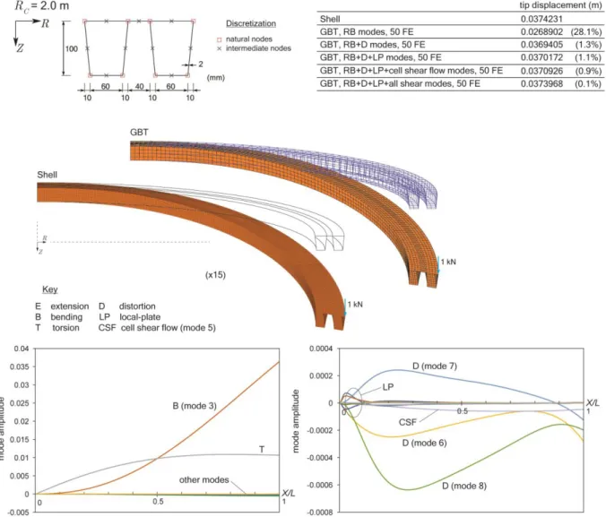
4.3 Three-cell beam subjected to an out-of-plane load
A beam with the three-cell cross-section presented in Fig. 4 is analyzed in this example (although the cross-section is discretized with more intermediate nodes, as shown in Fig. 7). The vertical force is applied at one corner of the free end cross-section, as shown in Fig. 7. The GBT analyses were carried out with several combinations of mode sets: (i) rigid body (RB, including the cell shear flow mode associated with torsion), (ii) Vlasov distortional (D) and (iii) local-plate modes (LP).
Figure 7: Three-cell section 90º cantilever beam subjected to an out-of-plane tip load.
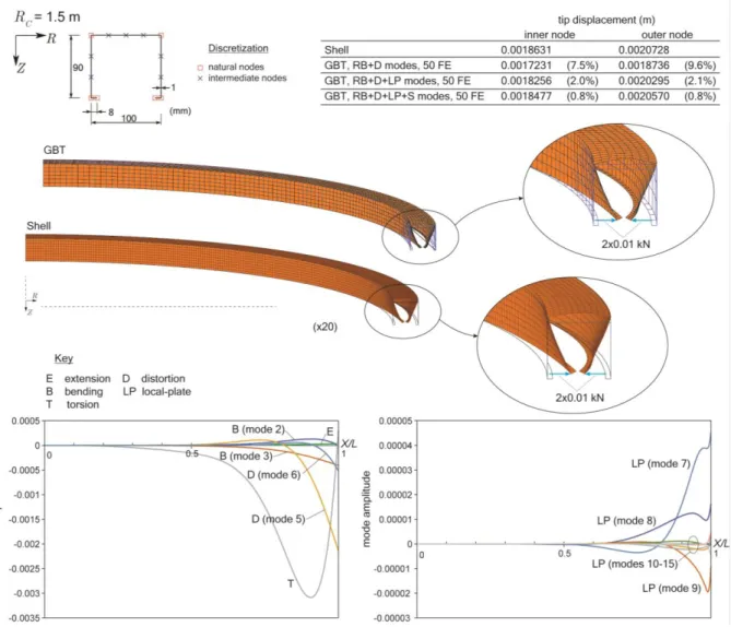
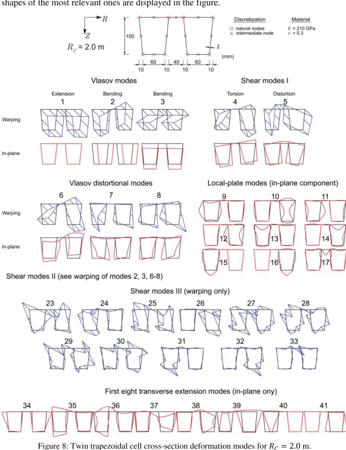
4.4 Twin trapezoidal cell beam subjected to an out-of-plane tip load
This final example consists of a twin trapezoidal cell section taken from [19]. Fig. 8 displays the cross-section geometry and discretization, leading to a total of 51 deformation modes – the shapes of the most relevant ones are displayed in the figure.
Figure 8: Twin trapezoidal cell cross-section deformation modes for 𝑅𝐶 = 2.0 m.
do not provide accurate results. In particular, the three Vlasov D modes (6-8 in Fig. 8) play a significant role. When either (i) all the LP (9-17) or (ii) the distortional cell shear flow (5) or (iii) all the shear modes are considered in the analysis, a small improvement in the results is obtained. The deformed configurations demonstrate clearly the excellent match between the shell and GBT models. The bottom-left modal participation graph shows that the B and T modes are dominant. Nevertheless, the Vlasov D modes are also quite relevant throughout the beam length, as shown in the bottom-right graph, followed by the cell shear flow mode 5. The LP modes are only relevant near the fixed end.
Figure 9: Three-cell section 90º cantilever beam subjected to an out-of-plane tip load.
5 CONCLUSION
This paper presented an improvement of the first-order GBT formulation for naturally curved thin-walled members introduced in [6], by proposing a systematic procedure to obtain the cross-section deformation modes for arbitrary flat-walled cross-sections (open, closed or
modes, particularly the rigid-body, Vlasov distortional and local-plate modes, and (ii) the modal features of GBT provide in-depth insight into the structural behavior of naturally curved bars.
ACKNOWLEDGEMENTS
The first author gratefully acknowledges the financial support of FCT (Fundação para a Ciência e a Tecnologia, Portugal), through the doctoral scholarship SFRH/BD/120062/2016.
REFERENCES
[1] Schardt R., “Eine erweiterung der technischen biegetheorie zur berechnung prismatischer
faltwerke”, Stahlbau, 35, 161-171, 1966 (German).
[2] Schardt R., Verallgemeinerte Technische Biegetheorie, Springer Verlag, Berlin, 1989 (German). [3] Camotim D., Basaglia C., Bebiano R., Gonçalves R., Silvestre N., “Latest developments in the GBT
analysis of thin-walled steel structures”, Proceedings of International Colloquium on Stability and Ductility of Steel Structures, E. Batista et al. (eds.), Rio de Janeiro, Brazil, 33-58, 2010.
[4] Camotim D., Basaglia C., Silva N., Silvestre N., “Numerical analysis of thin-walled structures using generalised beam theory (GBT): Recent and future developments”, Computational Technology Reviews, B. Topping et al. (eds.), Saxe-Coburg, Stirlingshire, 315-354, 2010.
[5] Camotim D., Basaglia C., “Buckling analysis of thin-walled steel structures using Generalized Beam Theory (GBT): state-of-the-art report”, Steel Construction, 6(2), 117-131, 2013.
[6] Peres N., Gonçalves R., Camotim D., “First-order Generalised Beam Theory for curved thin-walled members with circular axis”, Thin-Walled Structures, 107, 345-361.
[7] Winkler E., Die Lehre von der Elasticitaet und Festigkeit, H. Dominicus, Prague, 1868 (German). [8] Vlasov V., Tonkostenye Sterini, Fizmatgiz, Moscow, 1958 (Russian).
[9] Peres N., Gonçalves R., Camotim D., “GBT-based cross-section deformation modes for thin-walled members with circular axis”, Thin-Walled Structures, 127, 769-780, 2018.
[10] Gonçalves R., Ritto-Corrêa M., Camotim D., “A new approach to the calculation of cross-section deformation modes in the framework of Generalized Beam Theory”, Computational Mechanics, 46(5), 759-781, 2010.
[11] Gonçalves R., Bebiano R., Camotim D., “On the shear deformation modes in the framework of Generalized Beam Theory”, Thin-Walled Structures, 84, 325-334, 2014.
[12] Bebiano R., Gonçalves R., Camotim D., “A cross-section analysis procedure to rationalise and automate the performance of GBT-based structural analyses”, Thin-Walled Structures, 92, 29-47, 2015.
[13] Gonçalves R., Camotim D., “Generalised Beam Theory-based finite elements for elastoplastic thin-walled metal members”, Thin-Walled Structures, 49(10), 1237-1245, 2011.
[14] Gonçalves R., Camotim D., “Geometrically non-linear Generalised Beam Theory for elastoplastic thin-walled metal members”, Thin-Walled Structures, 51, 121-129, 2012.
[15] Dabrowski R., Gekrümmte dünnwandige Träger. Theorie und Berechnung, Springer-Verlag, Berlin/Heidelberg/New York, 1968.
[16] Oden J. T., Mechanics of Elastic Structures, McGraw-Hill, 1967.
[17] MATLAB, version 7.10.0 (R2010a), The MathWorks Inc., Massachusetts, 2010. [18] Bathe K. J., ADINA System, ADINA R&D Inc., 2017.