First-order Generalized Beam Theory for Curved Members
with Circular Axis
Nuno Peres1, Rodrigo Gonçalves2 and Dinar Camotim1 Abstract
This paper presents a first-order Generalized Beam Theory (GBT) formulation for thin-walled members with circular axis and undergoing complex global-distortional-local deformation. The fundamental equations are derived on the basis of the usual GBT kinematic assumptions (Kirchhoff, Vlasov and wall in-plane inextensibility), leading to a formulation able to retrieve accurate solutions with only a few cross-section deformation modes (cross-section DOFs). It is shown that the classic Winkler and Vlasov theories can be recovered from the derived formulation. A GBT-based finite element is use to analyze numerical examples illustrating the application and potential of the proposed formulation. 1. Introduction
Generalized Beam Theory (GBT) is a thin-walled prismatic bar theory that incorporates cross-section in-plane and out-of-plane (warping) deformation, through the consideration of “cross-section deformation modes” (cross-section DOFs), whose amplitudes along the member axis constitute the problem unknowns. GBT was introduced by Richard Schardt (1966, 1989) and has been continuously developed since then (Camotimet al. 2010, Basaglia & Camotim 2013) it is presently widely recognized as a very efficient tool to solve prismatic thin-walled member problems, due to its ability to (i) obtain accurate and structurally enlightening solutions with just a few deformation modes and (ii) include or exclude specific behavioral features in a straightforward manner. In fact, GBT often leads to analytical or semi-analytical solutions, which make it possible to draw meaningful conclusions concerning the structural behavior of prismatic thin-walled members.
This paper presents a first-order GBT formulation for naturally curved thin-walled members with circular axis (without pre-twist) and undergoing global-distortional-local deformation. Although the analysis of curved members is significantly more complex
1 CERIS, ICIST, DECivil, Instituto Superior Técnico, Universidade de Lisboa, Av. Rovisco Pais, 1049-001 Lisbon, Portugal.
than that of straight bars, it is shown that the most remarkable features of the classic GBT are retained, namely that (i) accurate solutions are obtained with only a few deformation modes and finite elements, and (ii) the unique GBT modal decomposition can be employed to investigate the complex structural behavior of curved thin-walled members, as illustrated by the numerical examples presented in the paper. 2. First-Order GBT for Members with Circular Axis
Due to space limitations, only an overview of the derivation of the fundamental relations and equations is provided a detailed account can be found in Peres et al. (2016). Fig. 1 shows the global cylindrical (, Z, R) and local wall (x, y, z) coordinate systems for an arbitrary curved thin-walled member. The member axis arc-length X defines the arbitrary cross-section “center” C, lies on the Z = ZC horizontal plane and has curvature equal to 1/RC. Concerning the wall local axes, y and z define the mid-line and through-thickness directions, respectively, and x is concentric to X. The small-strain-displacement relations are first obtained in the global cylindrical axes (e.g., Reddy 2013) and then transformed to thelocalaxesusingtheangle.Then,usingR = r + z cos , where r is the mid-line radius (Fig. 1 shows R and r for an arbitrary point P), Kirchhoff’s thin-plate assumption (zz=z =yz =0) is enforced, which eliminates plate-like shear locking and allows writing the local displacements (u,v,w) in terms of the mid-line (or membrane “M”) ones,
), , ( ), , ( ) , ( , ) ( ) , ( cos ) , ( ) , ( , , y w w y zw y v v y r y w y u z y u u y M M M (1)
where the commas indicate derivatives (e.g., f,x = f/x), although the derivative with respect to the arc-length is indicated by a prime, i.e., ()' = ()/X. Next, = X/RC is employed and the usual GBT variable separation is used,
uM = uT(y)'
(X), vM = vT(y)(X), w = ) (y
T
w (X), (2) where u,v,w are column vectors containing the mid-line displacement components pertaining to each deformation mode k and the column vector collects their amplitude functions (the unknowns). The derivative ' appearing in uM is necessary to incorporate Vlasov’s assumption. The strains read
, ' '
' ξ Φ ξ Φ
Φ ξ Φ ξ T xy T yy T T
xx 11 13 , 21 , 32
(3)
2 2
,Fig. 1. Global and local (wall) axes for a naturally curved thin-walled beam
where ()M, ()B are membrane/bending terms, Ky = cos/RC, Kz =sin/RC are the curvatures along the local axes and =RC/r. Comparing Eqs. (3) with those obtained for straight bars (Gonçalves & Camotim 2011, 2012) shows that the latter have much less terms and 11 = 0, since the v, w displacements cause no longitudinal strains. The equilibrium equations may then be cast as
, , * x z y T T x z y xx xy yy xx Q Q Q Φ Φ Φ Q Q Q X X X X B E E G F F D C (5)where Xij are generalized stresses, B-G are GBT modal matrices and Qi are generalized external loads, given by
, ) 1 ( , ) 1 ( , ) 1 ( , ) 1 ( , , , ) 1 ( , ) 1 ( 11 11 2 13 11 2 21 11 2 13 21 2 2 32 32 1 2 2 1 13 13 2 21 21 2 dA R R E dA R R E dA R R E dA R R E dA R GR dA R R E dA R R E A T C A T C A T C A T C A T C T A T C A T C
ξ ξ ξ ξ ξ ξ ξ ξ ξ ξ ξ ξ ξ ξ G F E D D D D D D C B (6) , ) ( , , ) ( , ) ( 2 1 2 * Φ Φ X Φ X Φ Φ X Φ Φ X C F D D D E B F E G T T xx yy T yy xx (7) . , ) ( , ) ( , dA R R q dA R R q z dA R R q z zK A C z z A C y y y A C x y x
w Q w v Q w u uQ
In these expressions, A is the cross-section area, L is the beam axis length, E is Young’s modulus, is Poisson’s ratio, G is the shear modulus and qi are body forces. The Xxx resultants are associated with longitudinal normal stresses, whereas Xxy are shear stress resultants and Xyy reflect transverse normal stresses.
As in the classic GBT, besides Kirchhoff’s assumption, two additional strain constraints are enforced: (i) null wall transverse membrane extensions (Myy0) and (ii) Vlasov’s assumption (xyM0), generally acceptable for open sections. Both these constraints reduce the number of admissible deformation modes with no significant accuracy loss and, in particular, Vlasov’s assumption eliminates shear locking effects. Concerning the first constraint, it is concluded that the vk functions must be constant in each wall, as in the classic GBT. To avoid over-stiffness, the membrane and bending terms must be uncoupled, by taking R/RC r/RC = 1/ and replacing E/(12) by E in the membrane terms. Vlasov’s assumption leads to
. /
,y z k
k
k u Ku
v
(9)Although this constraint is more complex than that for straight members, together with the M 0
yy
assumption it turns out that the uk functions must be at the most linear in y, as in the classic GBT.
3. Rigid-Body Modes for Open Sections
The particular case of the so-called “rigid-body” (RB) modes (axial extension, bending and torsion) for open sections is now addressed. It is assumed that C coincides with the centroid/shear centre and that the cross-section principal axes are parallel to the global Z, R axes. For the in-plane case (coupled axial force and bending), consider external loads applied along the beam axis, namely distributed axial forces n, transverse forces pR and moments mZ, deemed positive according to the global axes. For the axial extension and bending modes (k = 1, 2, respectively), one obtains the classic relations, with the shear force eliminated from the equilibrium equations (e.g., Winkler 1868, Armero & Valverde 2012),
R z y Z x xy C xx Z xx C R z y x xy C xx xx p Q Q m Q X R N X M X k R p Q Q n Q X R N X N X k , , 0 , / , , 2 , / , , 0 , / , , 1 * 2 * (10) Z R Z C C R C m p M R N n R p N R N , 2 (11) , ,
2 r
C r Z C r C r EI R EI M R EI R I A E
N
(12) , , , / ) ( 2 1 2 2 1 2
CXC CX C C CX C CR A C C r U R U R R U R U R r R r
where UC is the C displacement of C along the -axis and , stand for the axis extension and curvature.
For the out-of-plane case (torsion-bending coupling), vertical forces pZ and torsional moments mX distributed along the axis, one obtains the Vlasov (1958) equations for bending (k = 3) and torsion (k = 4),
, , 0 , , / , , 4 , , 0 , 0 , , , 3 * 2 * X z y x SV xy C R xx xx C X Z z y x xy C R xx R xx m Q Q Q T X R M X B X k R m p Q Q Q X R M X M X k (14) . , 2 X C R C X Z R C
R T m
R M R m p M R M (15) , , ,
B EI T GJ
EI
MR W SV (16)
,
, 2
2 2 1
1
C CZ C C C CZ R U R R R U (17)
where B is the bi-moment, TSV is the St. Venant torsion moment, T = B' + TSV is the total torsion, is the twist rotation, IW is the warping constant, J is the St. Venant torsion constant and is the torsion curvature.
4. Deformation Modes
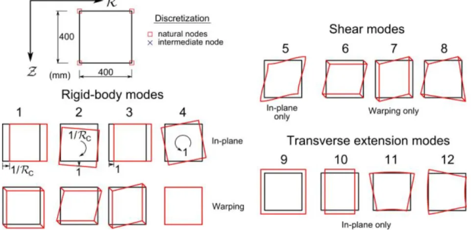
The present formulation can handle deformation modes involving any combination of the strain components in Eqs. (3). In particular, all the modes for straight members, as defined in Gonçalves et al. (2010, 2014), can be employed they can be calculated using the GBTUL software (Bebiano et al., 2015), freely available at www.civil.ist.utl.pt/gbt. However, note that the determination of the so-called “natural Vlasov modes” (warping modes complying with Vlasov’s assumption) requires special attention, as Eq. (9) differs from its straight bar counterpart. A two-step procedure is proposed, where (i) the warping functions are first calculated, using GBTUL, and (ii) the corresponding in-plane shapes are retrieved from Eq. (9), as in the classic GBT. Fig. 2 shows the deformation modes for a straight I-section member, based on the discretization indicated (6 natural nodes and a single intermediate node). For curved members, modes 5-21 are
retained, together with the warping functions of the Vlasov modes 1-4, which, in this
Fig. 2. Cross-section deformation modes for a striaght I-section member
Fig. 3. In-plane shapes of the rigid-body (Vlasov) modes for curved members
5. A GBT-Based Finite Element
and Lagrange quadratic functions, the latter for the deformation modes involving only warping displacements for further details, see, e.g., Gonçalves & Camotim (2012). Locking is mitigated by using reduced integration along X, with 3 Gauss points. In the mid-line direction y, the number of Gauss points between cross-section nodes generally depends on the mode types included in the analysis however, it was concluded that two points suffice in all the examples presented in the paper. It is assumed that R/RC 1/, whichuncouplesthemembrane/bendingtermsandmakesitpossibletoperform analytical integration along z. Finally, it is worth noting that the finite element procedure was implemented in MATLAB (The MathWorks Inc. 2010).
6. Numerical Examples
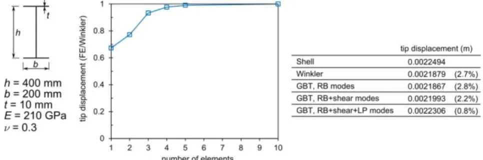
Allexamples concern 90º cantilever beams under free end section forces. For comparison purposes, classic Winkler and Vlasov theory solutions are provided, together with results obtained with refined shell finite element models, using ANSYS (ANSYS Inc. 2016). The displacement values reported are work-conjugate to each applied force. 6.1 In-Plane Bending of an I-Section Arch Beam
Consider the I-section beam displayed in Fig. 4. The graph plots the GBT-based displacement, obtained with the extension/bending modes and normalized with respect to the classic Winkler solution, as a function of the number of equal-length finite elements. As expected, the GBT results tend to the Winkler solution as more elements are used (<1% for >4 elements). The table compares the displacements obtained with a shell model with the Winkler solution and GBT results determined with 10 finite elements and several deformation mode sets: (i) RB modes 1-2, (ii) web-symmetric
shear modes 10 and 13-15 and (iii) the web-symmetric local-plate (LP) modes 8-9.
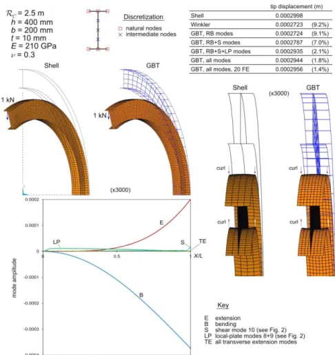
The Winkler and GBT-RB solutions fall almost 3% below the shell model value, due to cross-section deformation. This discrepancy is easily deal with in the GBT approach by including the shear (S) and LP modes, leading to a 0.8% difference. In order to examine further the effect of cross-section deformation, RC is decreased to 2.5 m and the results are shown in Fig. 5. The GBT analyses involved a cross- section
Fig. 5. In-plane bending of an I-section arch beam with RC = 2.5 m
(bending), although there are visible participations of the LP modes 8 and 9 (the curve
corresponds to the sum of the two participations), evidencing the observed curling phenomenon. It is also noted that the shear mode 10 has a relevant participation near
the tip, due to the present of the concentrated force, and that the transverse extension modes play a minute role.
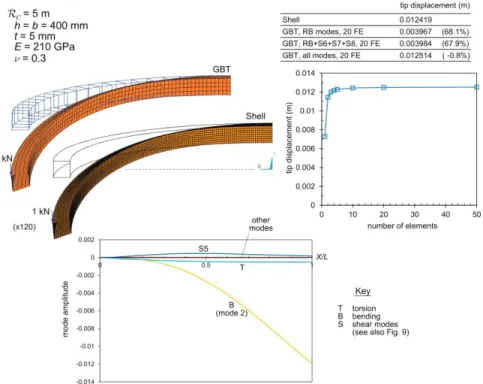
6.2 Out-of-Plane Bending of an I-Section Arch Beam
In this example, the force is applied, along Z, at the end section centroid (see Fig. 6). The GBT cross-section discretization involves a single intermediate node in the web, leading to the deformation modes 5-21 depicted in Fig. 2 and to the RB modes shown
in Fig. 3 (case b). The graph below the table in Fig. 6 plots the tip displacement, obtained with all deformation modes, against the number of finite elements considered. It is concluded that 10-20 elements lead to satisfactory results.
The deformed configurations displayed in Fig. 6 provide further evidence of the excellent agreement between the GBT and shell model solutions. However, it is noted that, in spite of the influence of the LP and S modes on the tip displacement value, their presence is, at best, barely visible. Further insight can only be provided by the mode amplitude graphs depicted at the bottom of the figure. The left graph makes it possible
to conclude that the bending and torsion modes are dominant their amplitudes are two orders of magnitude above those of the LP and S modes. The right graph shows a detailed view of the most relevant LP and S modes. It is observed that their amplitudes are mostly relevant near the support and that the LP modes 5 and 6 (flange rotation and
web transverse bending) are the most significant, even if the LP mode 7 (symmetric
transverse bending) and the bi-shear mode S12 also play non-negligible roles.
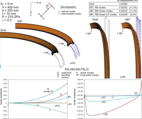
6.3 Arch Beam with a 45ºRotated I-Section
In this example, the beam cross-section is rotated by 45º and the load is applied, along the radial direction, at the lower flange-web junction see Fig. 7. The RB modes are shown in Fig. 3 (case c). The table in this figure makes it possible to compare the radial displacements of the point of load application obtained by means of a refined shell model and GBT with 20 finite elements and including various deformation mode sets. It is concluded that the GBT shear modes do not play a significant role also in this example (moreover, the transverse extension modes do not participate in the solution
this is not shown) and that very accurate results are obtained if the LP modes are included in the analysis. The deformed configurations displayed in Fig. 7 provide further
evidence of the good agreement between the shell finite element and GBT solutions. The two modal amplitude graphs depicted in the bottom of the figure provide additional relevant information. The four RB modes are predominant, with amplitudes several orders of magnitude above those of the LP modes nevertheless, as already shown, the LP modes are essential to obtain accurate tip displacement values. Finally, the r.h.s. graph shows that only the LP modes 5-7 have visible participations.
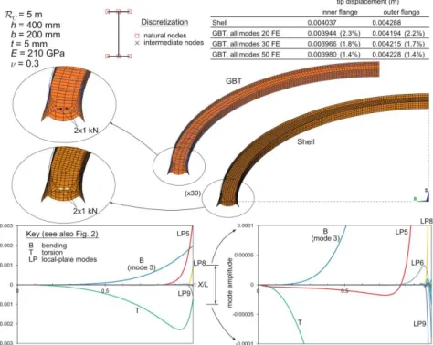
5.3 Local-Plate Bending of an I-Section Arch
Consider now that the arch acted by two self-equilibrated concentrated forces, as shown in Fig. 8. The GBT analyses are based on a cross-section discretization with no intermediate nodes, leading to 18 deformation modes they consist of the set shown in Fig. 2, excluding modes 7, 15 and 21 (for simplicity, the mode numbers in Fig. 2 are
kept), and the RB modes depicted in Fig. 3 (case b). The table in Fig. 8 displays the radial displacement of the points of load application, obtained with a refined shell model and GBT analyses including all 18 modes and various numbers of equal-length finite elements. The GBT solution with 20 elements is already quite close to the shell model one, but increasing the number to 50 brings the difference to a remarkable 1.4%. The deformed configurations depicted in the figure show, once more, the excellent
agreement between the two models, namely in the close vicinity of the beam free end the GBT deformed configuration was obtained with 30 elements.
The mode amplitude graphs provided in the bottom of Fig. 8 (at the r.h.s. one details the [0.0001, 0.0001] range) enable a clear visualization of the participation of all LP modes. Throughout the beam, the most significant participations are from the minor-axis bending (B3) and torsion (T) modes. Near the free end, the LP modes 5, 8 and 9
are also relevant, due to the concentrated force effects. The r.h.s. graph shows that the end section deformed configuration is rather complex contributions from many deformation modes (the unnumbered curves correspond to transverse extension modes). 6.4 Square Hollow Section Arch
The last example concerns the thin-walled square hollow section shown in Fig. 9. The GBT analyses are based on a cross-section discretization with no intermediate nodes (this particular example does not require such nodes), leading to 12 modes, whose in-plane shapes and warping functions are also displayed in Fig. 9. The first 3 RB modes comply with Vlasov’s assumption (for curved members). Since the cross-section is closed, the torsional mode (4) causes membrane shear deformation and does not
comply with Vlasov’s assumption for this reason, the mode shape for straight beams is considered. The shear modes comprise one in-plane distortional-type mode (5) and
three warping functions the first two (modes 6-7) correspond to those of modes 2-3.
Finally, 4 transverse extension modes are also obtained.
A cantilever arch beam is analyzed, loaded as shown in Fig. 10. The table in this figure provides the displacement values obtained with a refined shell model and GBT analyses with 20 equal-length finite elements and considering different deformationmodesets.Theseresultsshowthattheinclusion of the shear mode 5 is
absolutely essential to obtain the correct displacement value the difference with
Fig. 10. Square hollow section arch beam
respect to the shell model value drops from about 70% to less than 1%! The graph below the table plots the variation of GBT-based displacement, calculated with all deformation modes, with the number of finite elements. It is noted that 4 elements already lead to satisfactory results (difference with respect to the shell model below 2%), a feature that can be attributed to the fact that the cross-section deformation is not severely localized, as discussed below.
Fig. 10 also displays the deformed configurations obtained from both analyses and an excellent agreement is again observed. These configurations clearly show cross-section flattening occurring along the member. Finally, the deformation mode amplitudes are plotted in the bottom of Fig. 10. Clearly, modes 2 (bending), 4 (torsion) and 5 (shear) are the most relevant. In particular, and even though a
concentrated force is applied, it is observed that the amplitudes of modes 4 and 5
7. Concluding Remarks
This paper presented the development and validation of a first-order GBT formulation for naturally curved thin-walled members with circular axis (constant bending curvature). Attention is called to the following aspects of the proposed formulation: (i) It accommodates the standard GBT kinematic assumptions (Kirchhoff's, Vlasov’s
and null transverse membrane extensions), thus retaining the efficiency of the classic GBT. Moreover, shear and transverse extension modes can be also handled. (ii) The equilibrium equations may be written in terms of GBT modal matrices (the
standard approach) or stress resultants.
(iii)When particularized, the proposed formulation recovers the classic Winkler and Vlasov equations and fundamental relations.
(iv) A GBT-based finite element was implemented and employed to solve a set of representative numerical examples involving complex local-global deformation. In all cases it was concluded that accurate results are obtained with only a few deformation modes and finite elements. The GBT modal decomposition features wereshowntoprovidein-depthinsight on the structural behavior of curved members. Acknowledgements
The first author gratefully acknowledges the financial support of CERIS, granted through scholarship BL335/2015, from Project P469-S2/2-CC1152.
References
ANSYS Inc. (2016). ANSYS Release 16.2.
Armero F, Valverde J (2012). Invariant hermitian finite elements for thin Kirchhoff rods I: The linear plane case, Computer Methods in Applied Mechanics and Engineering 213-216, 427-457.
Bebiano R, Gonçalves R, Camotim D (2015). A cross-section analysis procedure to rationalise and automate the performance of GBT-based structural analyses, Thin-Walled Structures, 92(July), 29-47.
Camotim D, Basaglia C, Bebiano R, Gonçalves R, N. Silvestre (2010). Latest developments in the GBT analysis of thin-walled steel structures. Proceedings of International Coloquium on Stability and Ductility of Steel Structures(SDSS’2010 Rio de Janeiro, 8-10/9),E. Batista, P. Vellasco, L. Lima (eds.), 33-58.
Camotim D, Basaglia C (2013). Buckling analysis of thin-walled steel structures using Generalized Beam Theory: state-of-the-art report. Steel Construction, 6(2), 117-131. El-Amin F, Kasem M (1978). Higher-order horizontally-curved beam finite element including
Gonçalves R, Ritto-Corrêa M, Camotim D (2010). A new approach to the calculation of cross-section deformation modes in the framework of Generalized Beam Theory, Computational Mechanics, 46(5), 759-781.
Gonçalves R, Camotim D (2011). Generalised Beam Theory-based finite elements for elastoplastic thin-walled metal members, Thin-Walled Structures, 49(10), 1237-1245. Gonçalves R, Camotim D (2012). Geometrically non-linear Generalised Beam Theory for elastoplastic thin-walled metal members, Thin-Walled Structures, 51(February), 121-129. Gonçalves R, Bebiano R, Camotim D (2014). On the shear deformation modes in the framework of
Generalized Beam Theory, Thin-Walled Structures84(November), 325-334. The MathWorks Inc. (2010). MATLAB Version 7.10.0 (R2010a).
Peres N, Gonçalves R, Camotim D (2016). First-order Generalised Beam Theory for thin-walled members with circular axis, submitted for publication.
Reddy J (2013). An Introduction to Continuum Mechanics, Cambridge University Press.
Schardt R (1966), Eine erweiterung der technischen biegetheorie zur berechnung prismatischer faltwerke, Stahlbau, 35, 161–171. (German)
Schardt R (1989). Verallgemeinerte Technische Biegetheorie, Springer Verlag, Berlin. (German) Vlasov V (1958). Tonkostenye Sterjni, Fizmatgiz, Moscow. (Russian)