FUNDAÇÃO GETULIO VARGAS ESCOLA DE
PÓS-GRADUAÇÃO EM ECONOMIA
Rafaela Nogueira
Essays on Health Economics
Rafaela Nogueira
Essays on Health Economics
Tese para obtenção do grau de doutor apresentada a Escola de
Pós-graduação em Economia
Área de concentração: Microencomia aplicada
Orientador: Cecília Machado Berriel
Ficha catalográfica elaborada pela Biblioteca Mario Henrique Simonsen/FGV
Carvalho, Rafaela M. Nogueira de.
Essays on health economics / Rafaela Magalhães Nogueira de Carvalho. – 2016.
68 f.
Tese (doutorado) - Fundação Getulio Vargas, Escola de Pós-Graduação em Economia.
Orientadora: Cecília Machado Berriel.
Inclui bibliografia.
1.Economia da saúde. 2. Cuidados médicos - Custos. 3. Obesidade em crianças. 4. Guarda de menores - Aspectos psicológicos. I. Berriel, Cecília Machado. II. Fundação Getulio Vargas. Escola de Pós-Graduação em Economia. III. Título.
The E¤ects of Smoking Bans on Birth Outcomes
Rafaela Nogueira
yFGV/EPGE
Valdemar Neto
zFGV/EPGE
AbstractThis paper studies the impact of smoking bans on birth outcomes in the U.S. We exploit time variation in the introduction of smoking bans across states using the Natality Detail File from 1990-2004. Our main …nding suggests that the imple-mentation of smokefree legislation in workplaces has had a positive impact on birth weight. This impact is, however, economically small. We do not …nd any e¤ect on other birth outcomes such as Apgar scores, probability of low birth weight or probability of pre-term birth.
Keywords: Smoking bans, birth outcomes. JEL Code: D62, J13, I38.
We are grateful for the comments made by Cecilia Machado, Gustavo Araújo, Francisco Costa, Humberto Moreira, Fernando Bignotto and Christiane Szerman.
1
Introduction
Currently in the U.S., 15% of the population smokes regularly. However, almost 85%
of non-smokers have detectable levels of tobacco chemicals in their body ‡uids.1 The
worldwide annual mortality burden has reached 5 million deaths from direct tobacco smoking and another 600,000 deaths attributable to the e¤ects of environment smoke (World Health Organization, 2012). Therefore, an important e¤ect of smoking is the harm it might cause to those who do not smoke. To deter smokers from smoking in public places and protect people from the e¤ects of passive smoking, the U.S. and many countries all over the world adopted smoking bans policies.
Low birth weight is one of the most relevant, non-desired, birth outcomes because of the impact in the future life of the baby. Studies have shown that low birth weight infants face higher risks than other infants do for a variety of health and developmental disorders (Paneth, 1995). While the vast majority of low birth weight children have normal outcomes, as a group they generally have higher rates of subnormal growth, illnesses, and neuro developmental problems (Hack et al., 1995). In addition, low birth weight signi…cantly increases the risk of infant mortality. The dollar cost of the resources used disproportionately to care for low birth weight children is one measure of the burden of low birth weight (Lewit et al., 1995).
In the 1970s, the U.S. implemented some restrictions on smoking in public places, government buildings and airplanes. These smoking restrictions limited but did not ban smoking in public places. During the 1990s, however, smoking bans became more strin-gent, with the imposition of total bans, i.e., 100% smokefree in workplaces, restaurants and bars. These were pioneered by municipalities and counties, mainly in California. By 2015, almost 65.1% of the US population is protected by total bans in workplaces, 77.4% in restaurants and 65.3% in bars.
The impact of smoking bans can have an ambiguous impact on birth outcomes. Adda and Cornaglia (2010) show that total smoking bans can displace smokers towards non-smokers. If this is the case, pregnant woman could have their health worsened due to passive smoking, and as a consequence, a worse birth outcome. Smoking bans can also displace smokers away from non-smokers. The result would be better birth outcomes. Eisner et al. (1998), for example, report that bartenders’ respiratory health improves after the establishment of total bans in bars due to a decline in environmental tobacco smoke.
In this paper, we investigate the impact of total smoking bans in workplaces, bars and restaurants on birth outcomes. We consider leisure places as the combination of bars and restaurants. Studying the population of newborns is not only important because of the well-recognized negative impact of smoking during pregnancy (Permutt and Hebel,
1989), but also for the nine-month window during which pregnant women may have been a¤ected by health-related interventions. We exploit time and state variation in the introduction of smokefree legislation across the US between 1990-2004. We take advantage of a continuous nationwide registry of all births, the Natality Detail File, to study the e¤ects of the smoking bans on several birth outcomes: birth weight, the probability of low birth weight, pre-term birth and APGAR score. The implementation of smoking bans in workplaces increases birth weight, although the impact is small economically. We do not …nd any e¤ect of bans on other birth outcomes.
A crucial concern in such an exercise is whether the smoking ban adoption timing will in‡uence results. We follow the literature (Evans and Ringel, 2009, Almond et. al., 2011, Bharadwaj et al., 2014) and consider exposure to smoking bans at three di¤erent timings: month of conception, …rst and second trimester of pregnancy. We expect the impact of the smoking bans to be strongest when the introduction of the smoking bans occurs in the month of conception because it is the timing with the biggest exposure for the fetus. The results still show that the implementation of smoking bans in workplaces increases birth weight, with small impact. Also we do not …nd any e¤ect of bans on other birth outcomes. Moreover, we investigate if smoking bans a¤ect fertility rates because it changes the pool of babies for which outcomes are measured. A change in fertility rates could introduce a potential bias to our analysis. The e¤ects of the smoking bans on fertility rates are not statistically signi…cant.
This paper contributes to the growing empirical literature that investigates the impact of smoking bans on birth outcomes (Briggs, 2009; Bharadwaj et al., 2014). We use the census of births, therefore, re‡ecting the entire U.S. population. Briggs (2009), however, also uses the census of births. The empirical strategy chosen by Briggs, a di¤erence-in-di¤erences estimation, uses about 60% of the U.S. population. Briggs uses a smaller amount of the American population because the birth …les connecting mothers to their place of residence only for counties with living persons with 100,000 or more people. We compute the percentage of the state population in a given time that is covered by a total ban, therefore, our dataset represents the entire U.S. population. Moreover, our analysis covers all types of bans: workplaces and leisure places (combination of bars and restaurants). Bharadwaj et al. (2014), in contrast, analyzes a 2004 law change in Norway that extended smoking restrictions to bars and restaurants, we …nds that children of female workers in restaurants and bars born after the law change saw signi…cantly lower rates of being born below the very low birth weight threshold and were less likely to be born pre-term. Our results go in the same direction as Bharadwaj et al. (2014). In the U.S, we …nd that the implementation of smoking bans in workplaces increases birth weight by 20.12 grams (g), which is economically small. We do not …nd any e¤ect on other birth outcomes.
An important lesson from our analysis is that, although economically small, the impact of total smoking bans in bars and restaurants is statistically signi…cant. Along with others studies like Briggs (2009), Markowitz et al. (2011) and Bharadwaj et al. (2014), our paper underscores the importance of public policy regarding smoking and thereby a¤ecting, even if with minimum impact, birth outcomes.
The remainder of the paper is structured as follows. Section 2 shows the literat-ure review. Section 3 discusses the smoking bans in the USA. Section 4 describes the data and Section 5 presents our econometric speci…cation and results. Finally, Section 6 summarizes our main …ndings and concludes.
2
Literature Review
There is a vast literature on the deleterious e¤ects of maternal smoking during pregnancy on a variety of birth outcomes, including low birth weight, preterm birth, intrauterine growth retardation and spontaneous abortion. These adverse e¤ects are widely docu-mented (see Sexton and Hebel 1984; Shipp, Croughan-Minihane et al. 1992; Strauss and Pollack, 2001).
Smoking cessation early in pregnancy has been associated with a reduction in the risk of adverse outcomes (Vardavas, Chatzi et al. 2010). Even delayed cessation of smoking during the second or third trimester of pregnancy can reduce the adverse e¤ects of smoking during pregnancy (Lieberman, Gremy et al., 1994; Raatikainen, Huurinainen et al., 2007; Yan and Groothuis, 2013).
The impact of smoking bans on smoking behavior has also been studied. Evans et al. (1990) suggest that workplace bans reduce smoking prevalence by 5 percentage points and daily consumption among smokers by 10 percent. Anger et al. (2011) show that the introduction of smokefree legislation in Germany did not change average smoking behavior within the population. However, their estimates point to important heterogeneous e¤ects. Individuals who go out more often to bars and restaurants did adjust their smoking behavior. Following the ban, they became less likely to smoke and also smoked less. Adda and Cornaglia (2010) indicate that smoking bans perversely increase non-smokers’ exposure by displacing smokers to private places where they contaminate non-smokers.
Another part of the literature has evaluated the e¤ects of tobacco control policies on smoking and birth outcomes. The majority of studies have focused on the impact of changes in cigarette prices. Some authors found that U.S. pregnant women responded signi…cantly to increases in cigarette excise taxes, and that smoking during pregnancy reduced birth weight and doubled the risk of low birth weight (Evans and Ringel 1999, Ringel and Evans 2001, Lien and Evans 2005). Other authors have also found that the price elasticity of smoking participation is higher among pregnant women than in the
general population (Gruber and Koszegi 2001, Colman, Grossman et al. 2003).
In a closely related work, Briggs (2009) suggest that less-restrictive bans may do more to improve birth outcomes than total bans. In general, his results suggest some small but signi…cant impacts of smoking bans on weeks of gestation. Bharadwaj et al. (2014) was able to identify mothers who worked in restaurants and bars during the introduction of the smoking bans and found out that mothers a¤ected by the law had children with overall better health. Our work is distinguishable because we also consider workplace bans in our analysis. We also use a alternative explanatory variable such as percentage of the population covered by smoking bans instead of a dummy variable, which allows us to have more variability in the estimation.
3
The Smoking Bans in the USA
In the 1970s the …rst law requiring some restrictions on smoking in public places, gov-ernment buildings and airplanes was implemented. This law limited but did not ban smoking in public places. Arizona became the …rst state to have some smoking bans in public places in 1973. During the 1970s and the 1980s, smoking bans were increasingly imposed, usually by requiring separate areas for smokers and non-smokers. By 1986, 41 states in the U.S. and the District of Columbia had statutes restricting smoking to some extent. These bans, however, were not as strong or extensive as most bans currently in place: “During the 1990s, smoking bans became more stringent, with the imposition of total bans in workplaces, public places, restaurants and bars. These were pioneered by mu-nicipalities and counties, mainly in California in the early 1990s”(Adda and Cornaglia, 2010).
According to the American Non Smokers’ Rights Foundation, in 1995, Utah was the …rst state to require total bans in restaurants, i.e., 100% smokefree in restaurants. Which also means, not allowing even for smoking in attached bars or separately ventilated rooms. With an increasing body of evidence demonstrating the adverse health e¤ects of secondhand smoke, state and local governments across the country enacted an increasing
number of more restrictive bans during the 1990s.2
In the late 1990s and early 2000s, some states implemented total bans that prohibited smoking in most workplaces and all public places, including previously exempted bars and restaurants. In the 2000s, year after year the states started to ban smoking completely. According to American Non Smokers’Rights Foundation in 2015 there are 24 states with total bans in workplace, bars and restaurants. There are 29 states with total bans in
workplace, 35 states in restaurants and 30 states in bars.3
2For further information see The Respiratory Health E¤ects of Passive Smoking: Lung Cancer and
Graphs (1) and (2) show the prevalence of total bans in workplace and leisure places bans in California (CA), Utah (UT), Massachusetts (MA) and all the USA states between
1990-2004.4 We chose California because was the …rst state to have a percentage of
its population under total smoking bans in workplaces and leisure places. Moreover, Utah was the …rst state to require total smoking bans in leisure places in 1995. Also, Massachusetts was the second state to have a percentage of its population under total smoking bans in workplaces and leisures places. Therefore, we chose states with the biggest part of its population under total bans whether in workplace or leisure places.
Lines in Graph (1) shows the prevalence of workplace smoking bans. In 1990, 5% of the population of California was under total smoking bans in workplaces. By 2004, this number jumped to almost 40%. The population of Massachusetts begin to have workplace smoking bans in 2003, with 1,6% of its population being a¤ected. By 2004, Massachusetts had 2,2% of its population under workplace total bans. In 1990, 0.62% of the USA population was under the workplace smoking bans. By 2004, 5.62% of the American population was under workplace smoking bans. The population of Utah was not exposed to workplace smoking bans during the chosen period.
Lines in Graph (2) shows the prevalence of leisure places smoking bans. In 1990, only 0.1% of the population of California was exposed to leisure places smoking bans, and by 1998, the whole state was exposed. In 1995, the whole state of Utah was exposed to leisure places smoking bans. The population of Massachusetts begin to have leisure place smoking bans in 2000, with 1,2% of its population being a¤ected. By 2004, Massachusetts had 2,2% of its population under leisure places total bans. In 1990, 0.01% of the USA population was under the leisure places smoking bans. By 2004, 13.73% of the American population was under leisure places smoking bans.
4
Data and Descriptive Statistics
The data for our analysis is the combination of two main sources. The birth records come from the Natality Detail File and the date of the smoking bans introduction comes from the American Non Smokers’Rights Foundation. These two datasets are merged by state identi…ers.
The Natality Detail File from National Center for Health Statistics is a census of births in the United States. The Natality data are taken directly from birth records and contain information regarding birth outcomes, demographic characteristics, and since 1968, self-imputed maternal smoking. We use demographic data variables, for example, date of birth, place of residence, age, race and educational attainment of parents between
E¤ ects: Making Sense of the Evidence (2010) or Americans Non Smokers’ Right Foudation
1990-2004.5 The health data include birth weight and gestation in weeks.
We also use the precise date of the introduction of smoking bans which comes from the American Non Smokers’ Rights Foundation. They collect the date of introduction of smoking bans, whether these bans were introduced at city, county or state level. All the dates pertain to the introduction of total ban in workplaces, bars or restaurants. As mentioned before, we create leisure place smoking bans which is the combination of bars and restaurants smoking bans.
The birth …les connect mothers to their place of residence only for counties and muni-cipalities with living persons with 100,000 or more people; which represents almost 60% of the US population. In order to deal with the fact that we cannot connect all mothers to their place of residence, we aggregate bans at state level computing the percentage of the population in a given time that is covered by a total ban at workplaces or leisure places. In order to illustrate, suppose that a total ban in bars (restaurants) takes place in a county that represents 5% of a state population. So, 5% of this state population is under a total ban in leisure places. Suppose again that another total ban is adopted in bars and restaurants simultaneously in a county that represents 1% of a state population. Thus 1% of the state population in under a total ban in leisure places. The counties and states population come from the 2010 census.
The Integrated Public Use Microdata Series (IPUMS-USA) and The Second National Health and Nutrition Examination Survey (NHANES II) are also used in this study on an auxiliar analysis about the adoption of bans. The timing of adoption of the smoking bans could be correlated with other determinants of changes in birth outcomes, for example. The IPUMS consists of more than …fty high-precision samples of the American population drawn from …fteen federal censuses. The NHANES II is a nationwide probability sample of 27,801 persons from 6 months to 74 years of age. Conducted from 1976-1980, the NHANES II focused on nutrition and health.
Table 1 provides descriptive statistics for all outcomes and explanatory variables. The average weight of a newborn is 3.3kg and 7.2% of them are delivered before 36 weeks. The mean of states population under total bans in workplaces is 3.9% and 7.0% in leisure places.
5The 2005 public use data from 2005-on does not include geographic detail due to restrictions imposed
by the states. This means that the 2005-on data does not include any geographic variables such as state, county, msa, etc.
5
Econometric Speci…cation and Results
5.1
Validating the Empirical Strategy
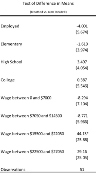
Our empirical strategy uses variation in when and where a total smoking ban was im-plemented to quantify the e¤ects on birth outcomes. The identi…cation of the e¤ects of regulation comes from variation across states and time, and not from cross-sectional dif-ferences in the level of state regulations, which are taken into account by state dummies. Our identi…cation relies on the exogeneity of changes in smoking bans regulations within states. We believe that the timing of establishment of the smoking bans is un-correlated with other determinants of changes in birth outcomes. To test whether this hypothesis is valid we collected several socio demographic characteristics and smoking habits of the state’s population from 1980. We examine whether characteristics between treated and non-treated states are di¤erent before the establishment of the smoking bans. The econometric model is:
Ys1980 = + T REATsk+ "s (1)
where Ys1980 represents a set of socio demographic characteristics and smoking habits of
the state s from 1980. The coe¢ cients and are the parameters to be estimated. The
variable T REATsk is a dummy variable that indicates whether the state s was treated
or not for total smoking ban of type k, where k refers to workplaces or leisure places
separately. We consider three treatment variables letting xk
s(t)denote a state s population
under smoking bans of type k at time t. The "s is the error term. The …rst treatment
exposure is given by:
T REATsk(A) = 1 x
k
s(t) > 0 for some t
0 otherwise
Hence, a state s is considered treated when in sometime t there is a positive fraction of the state population under some kind of smoking bans k. The second treatment variable considered is: T REATsk(B) = 1 if x k s = 2004P t=1990 xk s 15 > x k 0 otherwise
in this case, a state s is considered treated when the temporal average of the state’s population fraction under some kind of smoking bans k is bigger than the panel average. Finally we also consider:
T REATsk(C) = 2004 …rst time t where x
k
s(t) > 0 if 9 t; xks(t) > 0
16 if xk
here we want to measure the time since 1990 until the smoking law was approved. Hence, if a state s at any time t has a positive fraction of its population under a smoking bans of type k than the variable receives value equals to the time it took from 1990 until the law was approved.
Table 2 show the results from Eq.(1) and there is no evidence that any socio demo-graphic characteristics and smoking habits of the states from 1980 can explain the
in-troduction of the smoking bans. The coe¢ cient of interest, , with little exception, was
not statistically signi…cant. The only exception was the variable education. For all three versions of treated variables the e¤ects of education could not be rejected at 1% level of signi…cance.
The results yield no evidence of correlation between the timing of adoption of smoking bans and states characteristics. The only exception is education, which is used as a control variable in our baseline regression.
5.2
Mains Results
Our empirical strategy exploits variation in the location of a total ban and the timing of their establishment:
Yi;s;t= 0+ wxworki;s;t 6+ lxleisurei;s;t 6 + s+ t+ s:t + X 0
i;s;t 1+ "i;s;t (2)
here, Yi;s;t is the birth outcome of individual i from state s on time of birth t. We
consider four types of birth outcomes: birth weight (in grams); probability of pre-term birth de…ned as being born before gestational week 36; probability of being born with low birth weight de…ned as being born with less than 2.5kg; and …nally, APGAR score. The APGAR score summarizes the health of newborn children and ranges from zero to
10. In words, the variable xwork
i;s;t 6 is the percentage of the population in a given state s
and time t 6 covered by a total smoking ban in workplaces six months before birth.
And xleisure
i;s;t 6 is the percentage of the population in a given state s and time t 6 that is
subject to a total ban in leisure places six months before birth.
The timing of introduction of total smoking bans in our baseline regression is 6 months before birth. If the smoking ban is introduced within the …rst trimester of pregnancy, we say that the fetus was a¤ected by the introduction of a total ban. A fetus exposed to a total ban from the second trimester or ahead is considered not a¤ected by a total ban in uterus. Therefore, a baby is considered treated if two things happen: …rst, the state of residence must have had introduced the smoking bans; second, the introduction of smoking bans must happen before the end of the …rst trimester of pregnancy.
For robustness checks we estimate di¤erent numbers of months that a fetus was
we include state …xed e¤ects to control for time-invariant di¤erences in smoking
preval-ence and smoking patterns between states. t is a set of year-month …xed e¤ects that
accounts for potential common time trends across states. st is the state-speci…c e¤ects
in order to account for trends in smoking habits that are correlated with the passage of smoking bans laws. X is a set of control variables such as race, age and educational
attainment of parents. The variable "i;s;t is the error term. Standard errors are clustered
at the state level.
Table 3 reports the e¤ects of total bans on birth outcomes. Columns (1)-(12) show the results for an OLS regression including state …xed e¤ects, year-month …xed e¤ects, state-speci…c trends, a set of mother’s age, race and educational attainment dummies. The results are divided into two categories: birth weight and other birth outcomes.
5.2.1 Birth Weight
Columns (1)-(4) in Table 3 show the results when the timing of implementation occurs until the end of the …rst trimester of pregnancy. Column (1) reports the result including only state …xed e¤ects and year-month …xed e¤ects. Column (2) includes state speci…c trends. Column (3) includes a set of mother’s age and race dummies. Column (4), which is our preferred speci…cation, presents the estimates with the set of mother’s educational attainment dummies. The impact of workplace smoking bans is 20.12g when the intro-duction occurs until the end of the …rst trimester of pregnancy. The impact of leisure places smoking bans is not signi…cant.
Columns (5) and (6) show the results when the timing of implementation occurs until the month of conception and until the end of the second trimester of pregnancy. The impact of total smoking bans in workplaces on birth weight, independently of the timing, is positive and signi…cant. The strongest e¤ect appears when the workplace smoking bans is introduced until the month of conception, with an impact of 21.28g. When the implementation arises until the end of the second trimester, which is the most accurate estimation, the impact is 19.07g. The introduction of total bans in leisure places is not signi…cant for birth weight independently of the timing of implementation.
5.2.2 Pre-Term Birth, Low Birth Weight and Apgar Score
Columns (7)-(9) in Table 3 report the results for the probability of pre-term birth. The in-troduction of a total ban in workplaces and leisure places is not signi…cant, independently of the timing of exposure to the total smoking bans.
Columns (10)-(12) also show the results for the probability of being born with low birth weight. Once again, the introduction of total bans in workplaces and leisure places is not signi…cant, independently of the timing of exposure.
remain unchanged. The introduction of total bans in workplaces and leisure places is once again not signi…cant, independently of the timing of exposure.
5.2.3 Workplace and Leisure Places Separately
We also estimate with the variables W ork and Leisure separately. Tables 4A and 4B present the result for W ork and Leisure separately. Columns (1)-(3) in Table 4A present the impact of exclusively workplace bans on birth weight. When we consider the …rst trimester of pregnancy and month of conception, the timing of exposure is always positive and signi…cant. The impact of smoking bans in leisure places, shown in Table 4B, is not signi…cant.
The results from the estimates with the variables pre-term birth, low birth weight and Apgar score are also reported in Tables 4A and 4B. The results indicate that the impact is not signi…cant for neither type of smoking bans and neither timing of exposure to the total smoking bans.
5.2.4 Impact of Smoking Bans on Fertility Rates
Finally, we test whether smoking bans may have changed fertility rates which could introduce a potential bias to our analysis. Smoking bans may a¤ect the fertility rates by disproportionately elevating the chances of the fetus’birth. If this is true, the selection mechanism could increase prematurity and, therefore, decrease birth weight, which could generate a negative bias towards birth outcomes.
We constructed a measure of monthly fertility for the American states between 1990 to 2004 in order to study the impact of smoking bans into fertility rates. We want to examine whether the fertility rates were a¤ected by the introduction of smoking bans.
F ERTs;t = wx
work
s;t 6+ lx leisure
s;t 6 + s+ t+ s:t + Xi;s;t0 1+ "i;s;t (3):
Here, in addition to the other indices, the fertility rate, F ERTs;t, is de…ned as births per
1,000 women ages 15-44. The numerator is from the natality data (births collapsed to state-month). The denominator is from SEERS which we can use to create the population
of women ages 15-44 by state-year for years 1990 to 2004.6 7
The timing of introduction of total smoking bans in our baseline regression the same as Eq. (2), i.e., 6 months before birth. If the smoking ban is introduced before the month of conception, we say that the mother was a¤ected by the introduction of a total ban. A mother exposed to a total ban from the month of conception or ahead is considered
6See National Cancer Institute http://seer.cancer.gov/popdata/download.html.
7We assume that the total number of women between ages 15-44 in each year is homogeneously
not a¤ected by a total ban. Therefore, the mother is considered treated if two things happen: …rst, the state of residence must have had introduced the smoking bans; second, the introduction of smoking bans must happen before the month of conception. We also estimate di¤erent numbers of months prior to birth in order to check whether there is a change in fertility rates. Following Almond et al. (2011), we estimate with 3 months, 9 months, 12 months, 15 months, 18 months and 21 months prior to birth.
The e¤ects of the smoking bans on fertility rates are not statistically signi…cant. The estimates, presented in Table 5, indicate that our results are not being negatively biased.
We also estimate Eq.(3) with the variables xwork
s;t and xleisures;t separately. The results
remain unchanged, i.e., the e¤ects of the smoking bans on fertility rates remains not statistically signi…cant.
5.2.5 Discussion
Since 1990 smoking bans became more stringent, with the imposition of total bans in workplaces, public places, restaurants and bars in the U.S. on an unprecedented nation-wide tobacco control campaign. In order to assess the impact of the smoking bans, we analyze American’s comprehensive nationwide registry of births, the Natality Detail File, during 1990-2004.
Our empirical strategy uses variation in when and where a total smoking ban was implemented to quantify the e¤ects on birth outcomes. However, there may be trends in smoking habits that are correlated with the passage of smoking bans laws. Total bans may pass where smoking prevalence is declining, rather than the opposite causal interpretation. We attempt to address this concern by testing whether the timing of establishment of the smoking bans is uncorrelated with other determinants of changes in birth outcomes. The results show no evidence that the timing of the adoption of bans to be correlated with birth outcomes, except for education (which is included in our preferred speci…cation). We also include in the model, along with state …xed e¤ects, state-speci…c trends to account for possible endogeneity in the adoption of the smokefree laws.
In our econometric analyses, the smoking bans in workplaces is responsible for an increase of 20.12g in birth weight, when the introduction occurs until the end of the …rst trimester. Although positive, the impact is economically small. The impact of smoking bans in leisure places is not signi…cant for birth weight. We also undertake a few robustness checks changing the timing of introduction to month of conception and second trimester. The results do no alter, i.e., only total bans in workplaces a¤ects the birth weight. The impact of workplace smoking bans in birth weight is 21.28g, when the introduction occurs until the month of conception and 19.07g, when the introduction occurs until the end of the second trimester. Smoking bans in leisure places again do not
a¤ect birth weight. The smoking bans, independently of the type, do not a¤ect the other birth outcomes: probability of being born pre-term, probability of being born with low birth weight and APGAR score. The results do not alter even when we apply robustness checks.
We hypothesize, based on the …ndings of Bharadwaj et al. (2014), that the impact of total bans on birth outcomes is small because second hand smoke exposure has little impact on birth outcomes. An important issue is the possible mechanisms through which the law change a¤ects birth outcomes. This is a natural and important question. However, our available data is quite limited to address this question. First, there is a large amount of non-responses to questions related to smoking during pregnancy, which is crucial to understand how those mechanisms would work. For instance, in our data set 22% of the observations lack a response to those questions. Second, as it is well known in the literature (e.g., Dietz et al., 2011) variables based on questions related to smoking during pregnancy are self-imputed, which can be problematic since they can be considerably underreport. Additionally, we are not able to distinguish whether the changes in birth outcomes arises speci…cally out of quitting smoking or through other, broader changes in the mother’s life style, eating healthier or getting more nutrients, for example. To the extent that the smoking ban induced an overall healthier life style the policy impact of the smoking ban on birth outcomes is still relevant.
On the one hand, pregnancy may increase a woman’s aversion to environmental risks which decreases the likelihood of us …nding positive e¤ects on birth outcomes. If pregnant women do not spend a lot of time in bars, for instance, bans on smoking in bars may have little e¤ect on their infant’s birth outcomes. Also, if women decrease their labor supply during pregnancy, workplace smoking bans may have a smaller e¤ect on their infant’s birth outcomes.
On the another hand, smoking bans may reduce the health costs of some behaviors, such as working or spending time in bars, which in turn negatively a¤ect birth outcomes. Smoking bans may also negatively a¤ect birth outcomes by crowding more smoking into private environments (Adda and Cornaglia, 2006). For pregnant women who live or socialize with smokers, a ban on smoking of any kind may lead their partner to smoke more in shared private environments. Unfortunately, in the reduced-form analysis we cannot identify the mechanisms through which the smoking bans a¤ect birth outcomes.
Although our results can be read as a small impact of the tobacco control campaign, we believe that this result can be viewed as a lower bound of central estimates for state ban e¤ects. It is important to keep in mind that several states had some kind of previous smoking coverage. The preexistence of less strict smoking laws may a¤ect the results. It is reasonable to assume that states with previous tobacco restrictions should have a smaller impact of the implementation of total smoking bans. Besides, a …nal concern is whether
smoking bans may have changed fertility rates, which would introduce a potential bias to our analysis. Smoking bans may a¤ect the fertility rates by disproportionately elevating the chances of the fetus’birth. If this is true, than more babies would be born earlier, which could generate a negative bias towards birth outcomes. The e¤ects of smoking bans on fertility rates are not signi…cant for all types of speci…cations. Our results do not seem sensitive to this concern.
An important lesson from our analysis is that although statistically signi…cant the impact of a total ban in birth weight is economically small. Along with others important studies like Briggs (2009), Markowitz et al. (2011) and Bharadwaj et al. (2014), our paper underscores the importance of public policy regarding smoking and thereby improving, even if with minimum impact, birth outcomes. Our data is quite limited regarding questions related to smoking during pregnancy. We are not able, therefore, to understand the mechanism through which maternal behavior a¤ects birth outcomes in the presence of total smoking bans.
6
Conclusions
This paper examines the impact of smoking bans on birth outcomes in the U.S.. We exploit time variation in the introduction of smoking bans across states using the Natality Detail File from 1990-2004. Although the implementation of smokefree legislation in workplaces increases birth weight, the impact is economically small. We do not …nd any e¤ect along other birth outcomes like APGAR scores, probability of low birth weight and probability of pre-term birth.
Our identi…cation relies on the exogeneity of changes in regulations within states. Empirical tests indicate that the timing of establishment is uncorrelated with other states characteristics. Moreover, smoking bans can a¤ect fertility rates by disproportionately elevating the chances of the fetus’ birth. The e¤ects of smoking bans on fertility rates are not signi…cant. Therefore, our results are not being negatively biased.
The pre-existence of less strict smoking bans laws may a¤ect the results. It is reason-able to assume that, states with previous tobacco restrictions should have a smaller impact of the implementation of total smoking bans. Therefore, our results can be thought as lower bound limit for the impact of total smoking bans on birth outcomes.
Our paper studies the importance of public policy regarding smoking and thereby improving, even if with minimum impact, birth outcomes. Our data is quite limited regarding questions related to smoking during pregnancy. It is important to keep in mind that, unfortunately, in the reduced-form analysis we cannot identify the mechanisms from the total smoking bans to birth outcomes. Further research is necessary to understand and perhaps estimate the transmission mechanism from total smoking bans through maternal
behavior and from maternal behavior through birth outcomes. REFERENCES
1. Adda, Jerome, and Francesca Cornaglia. "Taxes, cigarette consumption, and smoking intensity." The American Economic Review 96.4 (2006): 1013-1028.
2. Adda, J., & Cornaglia, F. (2010). The e¤ect of bans and taxes on passive smoking. American Economic Journal : Applied Economics, 2(1), 1-32.
3. Almond, D., Hoynes, H. W., & Schanzenbach, D. W. (2011). Inside the war on poverty: The impact of food stamps on birth outcomes. The Review of Economics and Statistics, 93(2), 387-403.)
4. Anger, S., Kvasnicka, M., & Siedler, T. (2011). One last pu¤? Public smoking bans and smoking behavior. Journal of Health Economics, 30(3), 591-601.
5. Behrman, J. R., & Rosenzweig, M. R. (2004). Returns to birthweight. Review of Economics and statistics, 86(2), 586-601.
6. Bharadwaj, P., Johnsen, J. V., & Løken, K. V. (2014). Smoking bans, maternal smoking and birth outcomes. Journal of Public Economics, 115, 72-93.
7. Briggs, R. J. (2009). Essays on the economics of indoor and outdoor environments. 8. Colman, G., Grossman, M., & Joyce, T. (2003). The e¤ect of cigarette excise taxes on smoking before, during and after pregnancy. Journal of Health Economics, 22(6), 1053-1072.
9. Dietz, Patricia M., David Homa, Lucinda J. England, Kim Burley, Van T. Tong, Shanta R. Dube, and John T. Bernert. “Estimates of Nondisclosure of Cigarette Smoking Among Pregnant and Nonpregnant Women of Reproductive Age in the United States.” Am. J. Epidemiol. (2011) 173 (3): 355-359.
10. Dolan-Mullen, P., Ramirez, G., & Gro¤, J. Y. (1994). A meta-analysis of ran-domized trials of prenatal smoking cessation interventions. American Journal of Obstetrics and Gynecology, 171(5), 1328-1334.
11. Eisner, M. D., Smith, A. K., & Blanc, P. D. (1998). Bartenders’respiratory health after establishment of smoke-free bars and taverns. Jama, 280(22), 1909-1914. 12. Evans, W. N., & Ringel, J. S. (1999). Can higher cigarette taxes improve birth
13. Hack, M., Klein, N. K., & Taylor, H. G. (1995). Long-term developmental outcomes of low birth weight infants. The future of children, 176-196.
14. Harris, J. E., Balsa, A. I., & Triunfo, P. (2015). Tobacco control campaign in Uruguay: Impact on smoking cessation during pregnancy and birth weight. Journal of health economics, 42, 186-196.
15. Horta, B. L., Victora, C. G., Menezes, A. M., Halpern, R., & Barros, F. C. (1997). Low birthweight, preterm births and intrauterine growth retardation in relation to maternal smoking. Pediatric and Perinatal Epidemiology, 11(2), 140-151.
16. Institute of Medicine. Washington, DC. (2010). Secondhand Smoke Exposure and Cardiovascular E¤ects: Making Sense of the Evidence. National Academies Press. 17. Kramer, M. S. (1987). Determinants of low birth weight: methodological assessment
and meta-analysis. Bulletin of the World Health Organization, 65(5), 663.
18. Lewit, E. M., Baker, L. S., Corman, H., & Shiono, P. H. (1995). The direct cost of low birth weight. The future of children, 35-56.
19. Lieberman, E., Gremy, I., Lang, J. M., & Cohen, A. P. (1994). Low birthweight at term and the timing of fetal exposure to maternal smoking. American Journal of Public Health, 84(7), 1127-1131.
20. Lien, D. S., & Evans, W. N. (2005). Estimating the impact of large cigarette tax hikes the case of maternal smoking and infant birth weight. Journal of Human resources, 40(2), 373-392.
21. Markowitz, S., Adams, E. K., Dietz, P. M., Kannan, V., & Tong, V. (2011). Smoking policies and birth outcomes: estimates from a new era (No. w17160). National Bureau of Economic Research.
22. Mick, E., Biederman, J., Faraone, S. V., Sayer, J., & Kleinman, S. (2002). Case-control study of attention-de…cit hyperactivity disorder and maternal smoking, al-cohol use, and drug use during pregnancy. Journal of the American Academy of Child & Adolescent Psychiatry, 41(4), 378-385.
23. Paneth, N. S. (1995). The problem of low birth weight. The future of children, 19-34.
24. Permutt, T., & Hebel, J. R. (1989). Simultaneous-equation estimation in a clinical trial of the e¤ect of smoking on birth weight. Biometrics, 619-622.
25. Raatikainen, K., Huurinainen, P., & Heinonen, S. (2007). Smoking in early gest-ation or through pregnancy: a decision crucial to pregnancy outcome. Preventive medicine, 44(1), 59-63.
26. Ringel, J. S., & Evans, W. N. (2001). Cigarette taxes and smoking during preg-nancy. American Journal of Public Health, 91(11), 1851-1856.
27. Sexton, M., & Hebel, J. R. (1984). A clinical trial of change in maternal smoking and its e¤ect on birth weight. Jama, 251(7), 911-915.
28. Shipp, M., Croughan-Minihane, M. S., Petitti, D. B., & Washington, A. E. (1992). Estimation of the break-even point for smoking cessation programs in pregnancy. American journal of public health, 82(3), 383-390.
29. Strauss, R. S., & Pollack, H. A. (2001). Epidemic increase in childhood overweight, 1986-1998. Jama, 286(22), 2845-2848.
30. USDHHS. How Tobacco Smoke Causes Disease: The Biology and Behavioral Basis for Smoking-Attributable Disease: A Report of the Surgeon General. Atlanta, GA: U.S.. Department of Health and Human Services, Centers for Disease Control and Prevention, National Center for Chronic Disease Prevention and Health Promotion, O¢ ce on Smoking and Health, 2010.
31. Vardavas, C. I., Chatzi, L., Patelarou, E., Plana, E., Sarri, K., Kafatos, A., ... & Kogevinas, M. (2010). Smoking and smoking cessation during early pregnancy and its e¤ect on adverse pregnancy outcomes and fetal growth. European journal of pediatrics, 169(6), 741-748.
32. Weitzman, M., Gortmaker, S., Walker, D. K., & Sobol, A. (1990). Maternal
Table 2
Version E1 Version E2 Version E3 Version E1 Version E2 Version E3
A B C A B C
Family members avg 0.06 -0.00 -0.00 0.12* 0.16 -0.01
% people living in rural area -0.01 0.04 0.00 0.00 -0.23 0.01
% Men 0.00 0.00 0.00 0.01 0.00 -0.00 % White -0.03 -0.02 0.00 -0.03 -0.08 -0.00 % Black -0.02 -0.07 0.00 -0.03 -0.05 0.01 % Hispanic 0.06** 0.02 -0.01** 0.06** 0.03 -0.01** % Married -0.00 0.00 0.00 -0.01 -0.02 0.00 % Elementary -0.00 -0.01 0.00 -0.01 -0.04* 0.00* % High School -0.01 -0.01 0.00 -0.02** -0.02 0.00* % College 0.02 0.02 -0.00 0.02* 0.05** -0.00** % Students 0.00 -0.00 -0.00 0.01* 0.02** -0.00** % Students -0.00 0.00 0.00 -0.00 0.01 -0.00 % Employed -0.01 -0.01 0.00 0.00 0.03 -0.00
% Into the labor force -0.28 -0.35 0.05 -0.14 -0.97* 0.07 % People working more than 40 hours (week) -0.00 -0.00 0.00 0.00 -0.01 0.00 % Woman in laber force -0.00 -0.00 -0.00 -0.01 0.00 0.00
Wage -56.00 -13.94 -10.24 440.04 690.28 -58.41
% People with wage less than 3000 0.01 0.01 0.00 -0.01 -0.03 0.00 % People with wage between 3000 and 6000 -0.00 -0.00 0.00 0.00 0.00 -0.00 % People with wage between 6000 and 9000 -0.00 -0.00 -0.00 0.00 0.00 0.00 % People with wage between 9000 and 12000 -0.00 -0.00 -0.00 -0.00 0.00 0.00 % People with wage superior than 12000 -0.00 0.00 -0.00 0.01 0.03 -0.00 Dependency ratio (old) -0.01 0.01 0.00 -0.04* -0.03 0.00 Dependency ratio (young) -0.00 -0.02 0.00 0.02 0.01 -0.00
Dependency ratio -0.01 -0.01 0.00 -0.02 -0.03 0.00
% People ever smoked more than 100 cigarretes -0.01 -0.02 0.00 0.01 -0.04 0.00
% Smokers -0.03 -0.04 0.00 -0.04 -0.07* 0.01
Daily avg cigarretes -1.32 -0.54 0.14 -2.51 -1.93 0.23 Health spending (%) from GDP -0.00 0.00 -0.00 -0.00 0.00 0.00 Dependency ratio = (people between 0 and 14 years plus people above 64 years)/(people between 15 and 64 years) Dependency ratio (old) = ( people above 64 years)/(people between 15 and 64 years)
Dependency ratio (young)= (people between 0 and 14 years)/(people between 15 and 64 years) Standard errors in parentheses
** p<0.01, * p<0.05 Dependent Variables
Workplaces Leisure Places Test of Difference in Means
Ta bl e 3 (1) (2) (3) (4) (5) (6) (7) (8) (9) (10) (11) (12) (13) (14) (15) W or kp la ces 100. 87* * 2. 10 8. 60 20. 12* 21. 28* 19. 07* * .00 .00 .00 -0. 00 -0. 00 -0. 00 -0. 01 -0. 01 -0. 01 (38. 88) (0. 00) (0. 00) (10. 61) (11. 57) (9. 25) (.00) (.00) (.00) (.00) (.00) (.00) (0. 01) (0. 01) (0. 01) Lei su res p la ces 7. 88 7. 24 5. 51 3. 96 4. 17 6. 19 -.00 -0. 00 -0. 00 -0. 00 -0. 00 -0. 00 -0. 00 -0. 00 -0. 00 (12. 02) (0. 00) (0. 00) (4. 28) (4. 59) (4. 67) (.00) (.00) (.00) (.00) (.00) (.00) (0. 00) (0. 00) (0. 00) St at e FE Yes Yes Yes Yes Yes Yes Yes Yes Yes Yes Yes Yes Yes Yes Yes Ye ar -m on th FE Yes Yes Yes Yes Yes Yes Yes Yes Yes Yes Yes Yes Yes Yes Yes No Yes Yes Yes Yes Yes Yes Yes Yes Yes Yes Yes Yes Yes Yes M ot he r' s: Yes Yes Yes Yes Yes Yes Yes Yes Yes Age No No Yes Yes Yes Yes Yes Yes Yes Yes Yes Yes Yes Yes Yes Ra ce No No Yes Yes Yes Yes Yes Yes Yes Yes Yes Yes Yes Yes Yes No No No Yes Yes Yes Yes Yes Yes Yes Yes Yes Yes Yes Yes Cons ta nt 3, 23 18, 30 18, 30 18, 30 18, 30 18, 30 0. 105 0. 106 0. 107 0. 082 0. 083 0. 084 8. 43 8. 43 8. 43 The da ta c om es fr om the N at al it y De ta il F il e and the A m er ic an N on Sm ok er s' R ig ht s Founda ti on fr om 1 99 0-20 04 . T abl e 3 di spl ay s the im pa ct of W or kpl ac es S m ok ing Ba ns a nd Le is ur e Pl ac es S m oki ng B ans on bi rt h out com es : bi rt h w ei ght , C ol um ns (1 )-(4 ); Pr te -T er m B ir th, C ol um ns (6 )-(9 ); Low B ir th W he ig ht , C ol um ns (1 0) -( 12 ); and AP G AR Sc cor e, C ol um ns (1 3) -( 15 ). Col um n (1 ) i nc lude s st at e and ye ar -m ont h fi xe d ef fe ct s. C ol um n (2 ) i nc lude s st at e spe ci fi c ti m e tr ends . C ol um n (3 ) i nc lude s ag e and ra ce dum m ie s. C ol um n (4 ), w hi ch is our pr ef er re d spe ci fi ca ti on, inc lude s Educ at iona l A tt am inm ent dum m ie s. C ol um ns (5 )-(1 5) inc lude s st at e and ye ar -m ont h fi xe d ef fe ct s, s ta te s pe ci fi c ti m e tr ends , a nd m ot he rs a ge , r ac e and educ at iona l a tt ai nm ent dum m ie s. T he S m ok ing B an ca n be im pl em ent ed at the Fi rs t T ri m es te r of P re gna nc y, S ec ond Tr im es te r of P re gna nc y and M ont h of C onc ept ion. No tes : P re -t er m bi rt h is de fi ne d as be ing bor n be for e ge st at iona l w ee k 36 . L ow bi rt h w ei ght is c ons ide re d be ing le ss tha n 25 00 g a t bi rt h. T he num be r of obs er va ti ons for pr e-te rm bi rt h, bi rt h w ei ght a nd low bi rt h w ei ght is 6 0, 23 7, 73 6; 6 0, 17 2, 85 1 and 60 ,1 72 ,8 51 re spe ct iv el y. R obus t s ta nda rd er ror s ar e in pa re nt he se s (* ** p< 0. 01 , * * p<0. 05, * p<0. 1) . Educ at iona l at tai nm en t St at e-sp ec if ic tr ends M ont h of conc ept ion Se cond tr im es te r of pr eg na nc y M ont h of conc ept ion Se cond tr im es te r of pr eg na nc y F ir st tr imes ter o f pr eg na nc y M ont h of conc ept io Se cond tr im es te r of pr eg na nc y F ir st tr imes ter o f pr eg na nc y Pe ri od X= Fi rs t t ri m es te r of pr eg na nc y M ont h of conc ept ion Se cond tr im es te r of pr eg na nc y F ir st tr imes ter o f pr eg na nc y Bi rt h We ig ht Pre -T erm B irt h Low B ir th We ig ht AP G AR The Im pa ct of a F ul l B an on B ir th Out com es (F ul l ba n i m pl em ent ed i n pe ri od X)
Ta bl e 4A (1) (2) (3) (4) (5) (6) (7) (8) (9) (10) (11) (12) Lei su re pl ac es 3. 51 3. 43 5. 92 -0. 00 -0. 00 -0. 00 -0. 00 -0. 00 -0. 00 -0. 00 -0. 00 -0. 00 (3. 79) (3. 92) (4. 26) (0. 00) (0. 00) (0. 00) (0. 00) (0. 00) (0. 00) (0. 00) (0. 00) (0. 00) Sta te FE Yes Yes Yes Yes Yes Yes Yes Yes Yes Yes Yes Yes Ye ar -m on th F E Yes Yes Yes Yes Yes Yes Yes Yes Yes Yes Yes Yes Yes Yes Yes Yes Yes Yes Yes Yes Yes Yes Yes Yes Yes M ot he r' s: Yes Yes Yes Yes Yes Yes Yes Yes Yes Yes Yes Age Yes Yes Yes Yes Yes Yes Yes Yes Yes Yes Yes Yes Ra ce Yes Yes Yes Yes Yes Yes Yes Yes Yes Yes Yes Yes Ed uc at io nal Yes Yes Yes Yes Yes Yes Yes Yes Yes Yes Yes Yes Cons ta nt 18, 30 18, 30 18, 30 0. 105 0. 105 0. 105 0. 082 0. 082 0. 082 8. 43 8. 43 8. 43 The da ta c om es fr om the N at al it y De ta il Fi le a nd t he A m er ic an N on Sm oke rs ' Ri ght s Found at ion fr om 1 99 0-2 00 4. T abl e 4 B di spl ays the im pa ct of L ei sur e Pl ac es Sm oki ng Ba ns on bi rt h o ut com es : bi rt h w ei ght , Col um ns (1 )-(3 ); P rt e-T er m Bi rt h, Col um ns (4 )-(6 ); L ow Bi rt h W he ight , Col um ns (7 )-(9 ); a nd A PG AR Sc cor e, Col um ns (1 0)-( 12 ). A ll r eg re ss ions inc lude s ta te a nd ye ar -m ont h fi xe d e ff ec ts , s ta te s pe ci fi c t im e t re nds , a nd m ot he rs a ge , r ac e a nd e duc at iona l a tt ai nm ent dum m ie s. T he Sm oki ng Ba n c an be im pl em ent ed a t t he Fi rs t T ri m es te r of Pr egna nc y, Se cond T ri m es te r of Pr eg na nc y a nd Mont h of Conc ept ion. N ot es : Pr e-t er m bi rt h is de fi ne d a s be ing bor n be for e g es ta ti ona l w ee k 3 6. L ow bi rt h w ei ght is c ons ide re d be ing le ss tha n 2 50 0 g a t bi rt h. T he num be r of obs er va ti ons for pr e-t er m bi rt h, bi rt h w ei gh t a nd lo w b irt h w ei gh t i s 60, 237, 736; 60, 172, 851 an d 60, 172, 851 re sp ect iv el y. R ob us t s ta nd ard e rro rs a re in p are nt he se s (* ** p <0. 01, * * p< 0. 05, * p< 0. 1) . St at e-sp ec if ic tr ends Se cond tr imes ter Fir st tri m es te r o f pr eg na nc y M ont h of conc ept io Se cond tri m es te r o f pr eg na nc y Se cond tr imes ter F ir st tri m es te r of pr eg na nc y M ont h of conc ept io Se cond tr imes ter Fir st tri m es te r o f pr eg na nc y M ont h of conc ept io Pe ri od X= F ir st tri m es te r of pr eg na nc y M ont h of conc ept io Bi rt h W ei ght Pre -T erm B irt h Low B ir th W ei ght AP G AR s co re The Im pa ct of L ei sur e Pl ac es Ba ns on Bi rt h O ut com es (F ul l ba n i m pl em ent ed i n pe ri od X)
Ta bl e 4B (1) (2) (3) (4) (5) (6) (7) (8) (9) (10) (11) (12) W or kp la ces 19. 56* * 20. 33* * 18. 54* * 0. 00 0. 00 0. 00 -0. 00 -0. 00 -0. 00 -0. 01 -0. 01 -0. 01 (9. 56) (9. 98) (8. 16) (0. 00) (0. 00) (0. 00) (0. 00) (0. 00) (0. 00) (0. 01) (0. 01) (0. 01) St at e FE Yes Yes Yes Yes Yes Yes Yes Yes Yes Yes Yes Yes Ye ar -m on th FE Yes Yes Yes Yes Yes Yes Yes Yes Yes Yes Yes Yes Yes Yes Yes Yes Yes Yes Yes Yes Yes Yes Yes Yes M ot he r' s: Yes Yes Yes Yes Yes Yes Yes Yes Yes Yes Yes Yes Age Yes Yes Yes Yes Yes Yes Yes Yes Yes Yes Yes Yes Ra ce Yes Yes Yes Yes Yes Yes Yes Yes Yes Yes Yes Yes Yes Yes Yes Yes Yes Yes Yes Yes Yes Yes Yes Yes Cons ta nt 18, 30 18, 30 18, 30 0. 105 0. 105 0. 105 0. 082 0. 082 0. 082 8. 43 8. 43 8. 43 The da ta c om es fr om the N at al it y De ta il F il e and the A m er ic an N on Sm ok er s' R ig ht s Founda ti on fr om 1 99 0-20 04 . T abl e 4B di spl ay s the im pa ct of W or kpl ac es S m oki ng Ba ns o n b ir th o ut co me s: b ir th we igh t, C ol umn s (1 )-(3 ); P rt e-Te rm B ir th , C ol umn s (4 )-(6 ); L ow B ir th Wh ei gh t, C ol umn s (7 )-(9 ); a nd A PGAR Sc co re , C ol umn s(1 0)-(1 2). A ll re gr es si ons inc lude s ta te a nd ye ar -m ont h fi xe d ef fe ct s, s ta te s pe ci fi c ti m e tr ends , a nd m ot he rs a ge , r ac e and educ at iona l a tt ai nm ent dum m ie s. T he S m ok ing B an ca n be im pl em ent ed at the F ir st T ri m es te r of P re gna nc y, Sec ond Tr im es te r of P re gna nc y and M ont h of C onc ept ion. N ot es : P re -t er m bi rt h is de fi ne d as be ing bor n be for e ge st at io na l we ek 3 6. L ow b ir th we igh t i s c on si de re d b ei ng l es s t ha n 2 50 0 g a t b ir th . Th e n umb er o f o bs er va ti on s fo r p re -t er m b ir th , b ir th we igh t a nd lo w b ir th we igh t i s 60,2 37,736 ; 60,17 2,851 a nd 60, 172,85 1 re sp ecti ve ly . R ob us t s ta nd ard e rro rs a re in p are nth es es (** * p<0. 01, ** p <0. 05, * p<0. 1) . Educ at iona l at ta inm ent St at e-sp ec if ic tr ends Fir st tr im es te r of pr eg na nc y M ont h of co nce pt io Se cond tr im es te r of pr eg na nc y F ir st tr imes ter o f pr eg na nc y M ont h of co nce pt io Se cond tr imes ter Fir st tr im es te r of pr eg na nc y M ont h of co nce pt io Se cond tr im es te r of pr eg na nc y Pe ri od X= F ir st tr imes ter o f pr eg na nc y M ont h of co nce pt io Se cond tr imes ter Low B ir th We ig ht AP G AR s co re Bi rt h We ig ht Pre -T erm B irt h The Im pa ct of Wor kpl ac e B ans on Bi rt h Out com es (F ul l ba n i m pl em ent ed i n pe ri od X)
Ta bl e 5 (1) (2) (3) (4) (5) (6) (7) (8) (9) (10) (11) (12) (13) (14) (15) (16) (17) (18) (19) (20) (21) W or kp la ces 0. 16 0. 15 0. 13 0. 14 0. 13 0. 14 0. 14 0. 16 0. 14 0. 13 0. 15 0. 15 0. 15 0. 16 -(0. 13) (0. 14) (0. 16) (0. 15) (0. 12) (0. 12) (0. 11) (0. 11) (0. 13) (0. 14) (0. 13) (0. 10) (0. 11) (0. 10) Lei su res p la ces 0. 00 -0. 02 -0. 01 0. 03 0. 08 0. 06 0. 08 -0. 05 0. 03 0. 03 0. 07 0. 11 0. 09 0. 10 (0. 13) (0. 10) (0. 11) (0. 13) (0. 14) (0. 11) (0. 10) (0. 10) (0. 08) (0. 08) (0. 11) (0. 13) (0. 10) (0. 09) St at e FE Yes Yes Yes Yes Yes Yes Yes Yes Yes Yes Yes Yes Yes Yes Yes Yes Yes Yes Yes Yes Yes Ye ar -m ont h FE Yes Yes Yes Yes Yes Yes Yes Yes Yes Yes Yes Yes Yes Yes Yes Yes Yes Yes Yes Yes Yes Yes Yes Yes Yes Yes Yes Yes Yes Yes Yes Yes Yes Yes Yes Yes Yes Yes Yes Yes Yes Yes The fe rt il it y r at e i s de fi ne d a s bi rt hs pe r 1 ,0 00 w om en a ge s 1 5-4 4. T he nu m er at or is fr om the na ta li ty d at a (bi rt hs c ol la ps ed t o s ta te -m on th). T he de no m ina tor is fr om SE ERS w hi ch w e ca n u se to c re at e t he po pu la ti on of w om en a ge s 1 5-4 4 by s ta te -ye ar for ye ar s 1 99 0 t o 2 00 4. T abl e 5 di spl ays the im pa ct of W or kpl ac e a nd L ei sur e P la ce Sm oki ng Ba ns on Fe rt il it y r at es . Al l r egr es si on s i nc lud e s ta te fi xe d e ffe ct s, ye ar m on th fi xe d e ffe ct s a nd s ta te s pe ci fi c t im e t re nd s. Col um ns (1 )-(7 ) r efe rs to W or kpl ac es a nd L ei sur e P la ce Sm oki ng Ba ns toge the r. Col um ns (8 )-(1 4) r efe rs to W or kpl ac es Sm oki ng Ba ns on ly. Col um ns (1 5)-(2 1) r efe rs to L ei sur e P la ce s Sm oki ng Ba ns on ly. Sm oki ng ba ns c an b e i m pl em ent ed 3 m on ths , 6 m on ths , 9 m on ths , 1 2 m on ths , 1 5 m on ths , 1 8 m on ths a nd 2 1 m on ths pr ior to b ir th N ot es : T he nu m be r of ob se rva ti on s i s 9 ,1 80 . T he c on st ant is 5 .8 4 for a ll r egr es si on s. Robu st s ta nd ar d e rr or s ar e in p ar en th es es . *** (p <0 .0 1, ** p<0 .0 5, * p<0 .1 ). 15 mo nth 18 mo nth 21 mo nth St at e-sp ec if ic tr ends 18 mo nth 21 mo nth 3 mo nth 6 mo nth 9 mo nth 12 mo nth 21 mo nth 3 mo nth 6 mo nth 9 mo nth 12 mo nth 15 mo nth 3 mo nth 6 mo nth 9 mo nth 12 mo nth 15 mo nth 18 mo nth Pe ri od X= W or kp la ces a nd Lei su res P la ces W or kp la ces Lei su re Pl ac es The Im pa ct of Sm oki ng Ba ns on Fe rt il it y Ra te s (Sm oki ng ba ns im pl em ent ed a s of X m on ths pr ior to b ir th)
Do the Unilateral Divorce Laws Cause Child Weight
Gain?
Rafaela Nogueira
yFGV/EPGE
Abstract
This paper studies the impact of unilateral divorce laws on child weight gain. I use di¤erence-in-di¤erences approach exploiting time and state variation in the adoption of the unilateral divorce law. I analyze a comprehensive nationwide health examination survey (NHANES I) during 1971–1974. The results show that expos-ure to unilateral divorce law leads to bigger Body Mass Index (BMI) for children between 2 and 18 years. However, according to the Center of Disease Control and Prevention (CDC), this weight gain is still under the normality patterns. Results indicate that for the speci…c age group of children between 7 and 18 years the exposure to unilateral divorce law leads to bigger BMI and bigger probability to be overweight. I also investigate the possibles transmission mechanisms for the increase in BMI.
Keywords: Unilateral divorce law, child health, child weight JEL Code: J12, J13
1
Introduction
In the 70’s, the USA witnessed a tranformation into the family unity that has been called the “Divorce Revolution”. The unilateral divorce— divorce that does not require the explicit consent of both partners— reached 28 American states until 1974. According to the National Vital Statistics Reports from Marriages and Divorces, while less than 20% of couples who married in 1950 ended up divorced, almost 50% of couples who married in 1970 did divorce. Approximately half of the children born to married parents in the 1970s saw their parents divorce, compared to only about 11% of those born in the 1950s. The unilateral divorce law (UD) has been perceived as negative for children, once the ease of divorce could lead to the breakdown of the traditional family. Indeed, there is a large literature in sociology, developmental psychology, and economics that documents the negative impact to children of divorced parents, both as children and then later as adults. Amato and Keith (1991), for example, report that children of divorce have more di¢ culty than children in intact families adjusting both socially and psychologically. Surveys show that children of divorce are more likely to exhibit antisocial and impulsive behavior. They are more likely to become delinquents (Matsueda and Heimer, 1987; Zill, Morrison, and Coiro, 1993), and to perform worse academically (Guidubaldi, Perry, and Cleminshaw, 1984).
In this paper, I investigate whether the UD a¤ects child weight gain. I use di¤erence-in-di¤erences approach using the variation resulting from the di¤erences in the timing of the adoption of UD across the adopting states. To assess the impact of UD on child weight gain, I analyze a comprehensive nationwide health and nutrition examination survey (NHANES I) during 1971–1974. According to the Center of Disease Control and Prevention (CDC) there is only one type of underweight (underweight type I) and two types of overweight (overweight and obese). I propose more two less extreme underweight measures (underweight types II and III), to have a more detailed description weight
distribution of children.1
My results show that the introduction of UD leads to lower probability of being underweight type II and higher Body Mass Index (BMI) for children between 2 and 18 years old. Children between 2 and 18 years that have been exposed to UD between 1 and 5 years have lower 0.06 percentage point (p.p.) chance to be underweight type II. When exposed for 6 or more years the probability to be underweight type II is lower by 0.15 p.p. and the probability to be underweight type III is lower by 0.38 p.p.. Moreover, the
1Overweight is de…ned as a BMI at or above the 85th percentile for their heigh and wheight and
below the 95th percentile for children and teens of the same age and sex. Obesity is de…ned as a BMI at or above the 95th percentile for children and teens of the same age and sex. Underweight type I is de…ned as a BMI at or below the 5th percentile, underweight type II is de…ned as a BMI at or below the 10th percentile, underweight type II is de…ned as a BMI at or below the 25th percentile for children and teens of the same age and sex.
BMI increases by 2.36 units when the child is exposed to UD for at least 6 years, which is 14.8% of the baseline BMI. The big picture is that after the introduction of the UD children are increasing their BMI but they still under a normal weight pattern according to the CDC. According to my proposed approach, however, there is evidence that the a¤ected children are getting healthier, once there is lower probability to be underweight type II after the introduction of UD.
I then turn to investigate possible transmission mechanisms from UD to BMI. First, there is the direct e¤ect, the e¤ect of UD on divorce. The UD can dissolve the marriage contract and, therefore, can be seen as a change in those marriage contracts already in place at the time of the reform. Second, marriage decisions could also change in response to UD. Selection into marriage could either be positive or negative. Couples of relatively low match quality are now willing to marry, reducing the average match quality of married couples and therefore increasing their marriage and divorce propensity (Alesina and Giuliano, 2007). Contradictorily, since UD undermines the role of marriage as a commitment device, couples with relatively low match quality no longer marry, which increases the average quality of married couples and, therefore, decreases the marriage and the divorce propensity (Matouschek and Rasul, 2006). A third possible mechanism are the changes in incentives for relationship-speci…c investments (children). Marriage can be thought of as a commitment device that cultivates cooperation and induces partners to make relationship-speci…c investments (Matouschek and Rasul, 2006). Finally, making divorce easier can change the nature of the bargaining relationships between husband and wife. If UD weakens the bargaining position of women within marriage, children may have been negatively a¤ected, independently of the occurrence of a divorce. But, if the opposite occurs, i.e, UD increases the bargaining position of women within marriage, children may have been positively a¤ected.
In order to address the …rst mechanism I examine both the impact on the likelihood that adults in childbearing age are divorced and the impact on other marital status that may be a¤ected by this shift in legal regimes. The results from this exercise indicate that divorce per is acting as a transmission mechanims from UD to child BMI. Even though the probability of being married is not a¤ected by the UD, it is important to note that, my results are capturing the contemporaneous e¤ect of UD. Therefore, I cannot rule out the role of marriage as a transmission mechanism in the long term.
In order to shut down the selection into marriage and relationship-speci…c investments mechanims, I study children between 7 and 18 years. This age group is mostly comprised of children born before the introduction of the UD, with marriage decisions taken before the UD comes into place. Children exposed to UD between 1 and 5 years have 0.08 p.p. lower chance to be underweight type II. Children exposed to UD for 6 or more years have higher BMI by 3.77 units, which is 25.8% of the baseline BMI, lower the probability
of being underweight type II by 0.08 p.p. and lower probability of being underweight type III by 0.15 p.p.. However, the probability of being overweight increases by 0.87 p.p. when exposed to 6 or more years to UD. The results can be considered mixed, once on the one hand, it indicates that children have lower chance to be underweight type II. And on the other hand, indicates that those same children have higher chance to be overweight. These …nding indicate that the total e¤ect of selection into marriage and marriage-speci…c investiment is positive (decreases the wheight of children) and greater than the total e¤ect of divorce per se and bargaining (increases the wheight of children). The literature on the e¤ects of UD on children is not extensive. Gruber (2004), using a sample of adults (25 to 50 years old) from the US Census data for the period 1960 to 1990, …nds that those who were exposed to the reform as children have lower educational attainments and lower family incomes, marry earlier but separate more often, and have higher odds of adult suicide. Delpiano and Giolito (2008) using Census data for the period 1960 to 1980, link children between ages 6 and 15 with their mothers. They …nd that, because of the reform, mothers are more likely to be below the poverty line, to be divorced and to have lower family income. At the same time, they …nd that children are less likely to attend a private school and, in the case of black children, more likely to be repeating a grade.
I extend the previous literature by analysing the impact of UD on child weight. Few papers (Yannakoulia, et. al., 2008; Kimbro, 2013; Biehl et. al., 2014) show evidence that children are at greater risk of being obese because they are living outside of an intact family. A central limitation of these studies, however, is that divorce is not an exogenous event with respect to other determinants of child outcomes. Moreover, I study the heterogeneity in the impact of the reform among children exploiting the di¤erences in the size of the exposure to UD and di¤erences in age at which the child faced the reform. With this speci…cation, I am also able to study potential transmission mechanisms from UD to the family and from the family to the child, depending on at which point of the child’s life the family has faced the reform.
This article proceeds as follows. In Section 2, I present literature review. Section 3 presents the history of UD. In Section 4, I discuss my data and empirical strategy. Section 5 presents the results and Section 6 presents a full discussion on the results, interpretation and mechanisms. Section 7 concludes the paper.
2
Literature Review
The beginning of the 70’the USA witnessed a rise in divorce rates. Initially, part of the literature (Peters, 1986) proposed that the UD implementation did not change divorce rates. The argument behind Peters’ conclusions is that the introduction of UD simply
represents the reallocation of an existing property right from one spouse to the other. According to the Coase theorem, a change in property rights does not change resource allocation but in‡uences the distribution of wealth. Therefore, the transaction costs should not be important for the study of marriage. Later on, another part of the literature suggested that the ease of divorce was a major contributing factor for the rapidly rise in divorce rates because it represented the breakdown of the traditional family structure (Douglas, 1992; Friedberg,1998). This …ndings has since been widely accepted until (Wolfers, 2006). He …nds that the divorce rate rose sharply following the adoption of unilateral divorce laws, but that this rise was reversed within about a decade. Therefore,
he claims that there is no evidence that the rise in divorce is persistent.2
Divorce has been perceived as negative for children since it represented a rupture of the tradicional family structure. Several studies have tried to identify the impact of easier divorce process on child outcomes. After reviewing 92 studies, Amato and Keith (1991) reported that children of divorced parents have more di¢ culty then children in intact families adjusting both socially and psychologically. Surveys show that children from divorced families are more likely to exhibit behavior that is antisocial or impulsive. They are more likely to become delinquents and they are more likely to perform worse academically (Matsueda and Heimer 1987; Zill, Morrison, and Coiro 1993).
The research on adolescents from divorced families also documents negative con-sequences. Adolescents with divorced parents are two to three times more likely to drop out of school, become pregnant, or engage in antisocial and delinquent behavior, and they score above clinical cuto¤s on standardized tests of behavior (Achenbach and Edelbrock 1983). These adolescents also begin to date and have sex at a younger age (Flewelling and Bauman 1990). Adolescents whose parents have divorced are more likely to have a low academic performance and to drop out of school, even after one controls for socioeconomic status (Guidubaldi et. al. 1984; Krein and Beller 1988).
A central limitation of these studies is that divorce not necessarily is an exogenous event with respect to other determinants of child outcomes. The exception are Gruber (2004) and Delpiano and Giolito (2008). Gruber points out that adults who were exposed to UD regulations as children are less well educated, have lower family incomes, marry earlier but separate more often and have higher odds of adult suicide. Delpiano and Giolito (2008) found that the unilateral divorce reform have negative e¤ects on child
2Wolfers (2006) explores several possible explanations. First, he explores dynamics, i.e., UD may
have simply led to the earlier dissolution of bad matches, thereby shifting a number of divorces from the 1980s into the 1970s. Second, there is matching. The quantity and quality of marriage market matches may change in response to divorce law changes. Moreover, there is contamination. An easier access to divorce in reform states may also reduce stigma in non-reform states, leading their divorce rates to rise, albeit with a lag. Finally, ther is the the regression to the mean. States with historically higher divorce rates were more likely to choose to reform their laws. Therefore, this suggests that convergence in divorce norms, or regression to the mean, may explain why divorce rates rose faster in control states, yielding