and D. Tian
1Department of Earth Sciences, School of Ocean and Earth Science and Technology, University of Hawai‛i at Mānoa,
Honolulu, HI, USA,2IDL, University of Algarve, Faro, Portugal,3EUMETSAT, Darmstadt, Germany,4Sea and Surf
Technology GmbH, Trappenkamp, Germany,5Laboratory for Satellite Altimetry, NOAA, College Park, MD, USA,
6Department of Earth and Environmental Sciences, Michigan State University, East Lansing, MI, USA
Abstract
The Generic Mapping Tools (GMT) software is ubiquitous in the Earth and ocean sciences. As a cross‐platform tool producing high‐quality maps and figures, it is used by tens of thousands of scientists around the world. The basic syntax of GMT scripts has evolved very slowly since the 1990s, despite the fact that GMT is generally perceived to have a steep learning curve with many pitfalls for beginners and experienced users alike. Reducing these pitfalls means changing the interface, which would break compatibility with thousands of existing scripts. With the latest GMT version 6, we solve this conundrum by introducing a new“modern mode” to complement the interface used in previous versions, which GMT 6 now calls“classic mode.” GMT 6 defaults to classic mode and thus is a recommended upgrade for all GMT 5 users. Nonetheless, new users should take advantage of modern mode to make shorter scripts, quickly access commonly used global data sets, and take full advantage of the new tools to draw subplots, place insets, and create animations.Plain Language Summary
The Generic Mapping Tools software is widely used in Earth and ocean sciences to process data and make maps and illustrations. This new version simplifies usage, adds quick access to key data sets, and provides a tool for making scientific animations.1. Introduction
The Generic Mapping Tools (GMT) have many tens of thousands of users worldwide. Most users around the world (approximately two thirds) use GMT under Windows (and with Ubuntu bash for Windows 10 gaining traction, this fraction may increase) followed by macOS and Linux, whereas in the United States the dominant operating system for GMT users appears to be macOS. GMT has been around for almost 30 years and it is embedded in many mission‐critical workflows. GMT is widely used in marine geology and geophy-sics (e.g., Müller et al., 2016), solid earth geophygeophy-sics (e.g., Ritsema et al., 2011), geodesy (e.g., McClusky et al., 2000), geodynamics (e.g., Steinberger et al., 2004), oceanography (e.g., Key et al., 2004), and planetary sciences (e.g., Smith et al., 1999). GMT is also a prerequisite foundation for other high‐level tools used by the scientific community, including MB‐System (Caress & Chayes, 1996) for multibeam bathymetry and backscatter processing and GMTSAR (Sandwell et al., 2011) for interferometric radar processing.
GMT version 1 wasfirst released informally in 1988 at Lamont‐Doherty Earth Observatory while the foun-ders Paul Wessel and Walter Smith were still in graduate school. At that time, the tools spread slowly as vis-iting scientists and graduating students took copies of the software with them on magnetic tape. Most users became familiar with GMT in 1991 when version 2.4.1 was released and announced via an article in EOS (Wessel & Smith, 1991). Minor updates were released a few times each year, while every few years, major new versions were released, such as GMT 3 (Wessel & Smith, 1995, 1998) and GMT 4 (2004, online announcement only). It took almost 10 years for the next major release [version 5; Wessel et al., 2013], as it included a major migration to a C‐language Application Program Interface (API).
With this article, we present and discuss the latest major release of GMT, version 6, which has been in devel-opment for 3 years. In many ways it is our most ambitious release as it seeks to strengthen GMT while retain-ing compatibility with the myriad of existretain-ing GMT scripts that have been written to date. At the same time, it seeks to break new ground in order to simplify how GMT can be used by new and experienced users alike. In order to accomplish these two goals GMT 6 now supports a“classic mode,” which runs exactly like GMT 5 and so offers full backward compatibility, and a“modern mode,” which allows new features and shorter and
© 2019. The Authors.
This is an open access article under the terms of the Creative Commons Attribution License, which permits use, distribution and reproduction in any medium, provided the original work is properly cited.
Key Points:
• A new version of the Generic Mapping Tools (GMT) is released • A new modern mode,
complementing the existing classic mode, greatly simplifies GMT scripting
• Easy access to remote data sets and advanced animation building facilitate science communication
Correspondence to:
P. Wessel, [email protected]
Citation:
Wessel, P., Luis, J. F., Uieda, L., Scharroo, R., Wobbe, F., Smith, W. H. F., & Tian, D. (2019). The Generic Mapping Tools version 6. Geochemistry, Geophysics, Geosystems, 20, 5556–5564. https://doi.org/10.1029/2019GC008515
Received 19 JUN 2019 Accepted 28 AUG 2019
Accepted article online 5 SEP 2019 Published online 1 NOV 2019
simpler scripts, so that GMT is now easier to learn. Our design challenge has been to make all of this seamless, backward compatible, and cross platform.
2. GMT Philosophy and Design
GMT began as a UNIX command‐line tool set. GMT modules were designed to mimic UNIX programs which act asfilters: Input is sent via standard input and output is returned via standard output. This design makes it easy to combine GMT (and other) processes by redirecting the output of one module as input to another. Output data may be composed by combining the results from several modules, using UNIX redirections to append various outputs to any one datafile. GMT employed this design for drawing illustrations as well as analyzing andfiltering data. Since plot-ting tasks were distributed across many modules, GMT modules needed to coordinate in order to produce a complex illustration. PostScript was GMT's graphics language from the beginning, and so GMT had to ensure that thefinal PostScript file, being an executable program with a particular syntax, was assembled in the correct order, regardless of how the GMT tools had been combined to create the illustration. This gave GMT the power offlexibility but also posed a challenge to users.
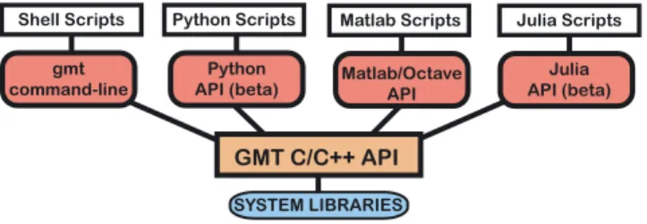
Individual GMT modules were coded as stand‐alone executables, just like UNIX programs. However, the release of GMT 5 (Wessel et al., 2013) introduced three key changes: (1) We provided a fully documented API for building new tools and libraries on top of GMT modules and functions. The API contains basic func-tionality for handling GMT data objects (i.e., the input/output of data), manipulating module options, reporting of errors and warnings, and accessing any of the ~120 modules. Unlike the previous GMT 4 ver-sion, these modules are no longer stand‐alone programs but are implemented as high‐level functions in the API. (2) We addressed issues with“namespace pollution”, that is, how to manage lots of different pro-gram executables in a standard installation directory (such as /usr/bin) when there might be many other tools with exactly the same names. For instance, there are already other software packages that distribute programs called“surface” or “triangulate” and that means they are competing for installation in the same directory as GMT when software is installed via standard software package managers. By building just a sin-gle executable called gmt (that we use to access all modules) and by requiring users to run“gmt triangulate” instead of just“triangulate”, we avoid this conflict. A few shell functions implement backward compatibility with older GMT 4 scripts that do not use the gmt executable. (3) We generalized the notion of input sources and output destinations. In addition to the familiar mechanism of passingfile names or using standard input/output, developers using the API can specify the sources of input and/or the destinations of output in several different ways, including memory locations,file pointers to open files or standard streams, and file descriptors. The GMT modules themselves are unaware of these distinctions since thisflexibility is imple-mented in the API input/output layer. Consequently, the new GMT API has made it possible for developers to build additional tools or external libraries on top of the core API (Figure 1). This change allowed for rapid development of new and complex functionality, such as discipline‐specific processing not presently available in the main GMT tool chest (e.g., Wessel et al., 2015).
At present, there are three lines of development using the GMT API: (1) The GMT/MATLAB Toolbox (Wessel & Luis, 2017) targets MATLAB users who want full access to GMT modules while working in the environments of MATLAB or Octave. (2) The PyGMT library (Uieda & Wessel, 2017) allows Python pro-grams to call GMT modules, including in interactive environments like the Jupyter notebook. (3) The GMT.jl package (Luis & Wessel, 2018) similarly allows Julia users access to GMT from its environment. The intertwined use of GMT, MATLAB, Python, and Julia encapsulates the modern working environments of major groups of scientists, especially those operating within the Earth, ocean and planetary sciences. While GMT continues to be predominantly used from a UNIX shell environment (such as Ubuntu bash for Windows 10, macOS, or a Linuxflavor like Ubuntu or CentOS), we expect this to change as the interac-tive environments provided via notebooks continue to improve and grow market share.
Figure 1. Conceptual block diagram of Generic Mapping Tools (GMT) dependencies. The high‐level functionality resides in the API, and modules are called via the single gmt executable. Supplemental and custom APIs may also be accessed this way. The GMT/MATLAB and GMT/Python APIs offer scripts written in those languages direct access to all GMT modules, similar to how UNIX shell scripts access modules via the gmt executable. The Julia and Python APIs are currently experimental.
3. Modern Versus Classic Mode
For almost three decades, GMT scripts written in new releases have looked remarkably similar to those writ-ten in earlier releases. The main option flags and the general workflow of adding overlays to existing PostScriptfiles have remained unchanged, and thousands of GMT scripts written in c‐shell, bash, DOS batch, and other environments exist and their maintainers expect them to run in the future. This require-ment of backward compatibility has, to some extent, stifled our desire to make GMT easier and safer to use. The dilemma is captured in the rallying cry from many a frustrated GMT user:“Make things simpler but don't change anything!” Having run dozens of courses introducing GMT to students and scientists and helped thousands of practitioners via email or user forums over the years, we have a clear idea of what is difficult about learning GMT. Given its almost limitless capabilities, GMT has always had a fairly steep learning curve. The hardest aspects that have percolated to the top of the pitfalls list include the following: (1) GMT“cake baking”: Handling the use of ‐O, ‐K, and ‐P to manage PostScript overlays; (2) The PostScript redirection: Creating a newfile versus appending to an existing file; (3) Reusing the current region (‐R) and projection (‐J) in multistep scripts by repeating the empty ‐R ‐J settings for every command; (4) Converting the PostScript plot to more desirable graphic formats, such as PDF; and (5) Positioning multipartfigures (e. g., a matrix layout) is a tedious and error‐prone operation.
While pondering these facts, we also started to gain experience with the GMT/MATLAB Toolbox and the ongoing design of the PyGMT library. We were noticing that the resulting scripts looked too similar to the GMT shell command‐line versions, setting users up for a continuation of the same pitfalls. We have decided that the best possible solution to this conundrum is to introduce different run modes that can be enabled by the user. Starting with GMT 6, we introduce a new operating mode for GMT named modern. In contrast to the classic(and only) mode available in earlier versions, modern mode was designed to eliminate some of the most challenging aspects of learning and using GMT. Depending on how a GMT script is started it will either be running in classic or modern mode. Classic mode is the GMT scripting style in use for decades and it will remain the default mode for command‐line work. In contrast, modern mode imposes simpler rules that elim-inate the possibility of the listed pitfalls; therefore, it promises to simplify scripting considerably across all interfaces. It also imposes a more rigid structure, and hence, not every single classic script may be represented using modern mode rules. Consequently, modern mode is slightly lessflexible but much easier to use, and we expect it will serve the needs of almost all GMT users. We will strongly encourage new users to use modern mode.
To defeat the pitfalls listed above, here are the key design features of modern mode: 1. The‐O, ‐K, and ‐P options are no longer needed nor available.
2. Plotting modules no longer write PostScript to standard output which users must redirect. Instead, they write to hidden temporaryfiles. GMT 6 checks the status of these files to know whether it is creating a new illustration or appending to an existing one.
3. In modern mode, the entire workflow runs in a unique temporary directory where its settings and history are kept. Hence, numerous scripts can execute simultaneously without interfering with each other, and we can use the history information to automatically supply missing region (‐R) and projection (‐J) arguments.
4. When the workflow ends, the hidden PostScript files are automatically completed and converted to the chosen graphics format, which defaults to PDF for command‐line work. In fact, more than one output format may be selected, for example, PDF and PNG.
5. Page size is now automatically determined regardless of map size and is properly cropped tofit from the initial (and maximum) canvas size of 32,767 × 32,767 points.
6. New modulesfigure, inset, and subplot automate the design and plotting of multiframe illustrations, while modules movie and events simplify animations. We will highlight these new modules in this paper. An example comparing a simple script written in both classic and modern modes is shown in Figure 2. Note how the show option to gmt end will display the plot in the default viewer program for the user's operating system.
Not only does modern mode significantly reduce the greatest obstacles to GMT learning, it greatly sim-plifies scripting by eliminating needless repetition of options and output filenames. Modern mode is acti-vated and deactiacti-vated by the new GMT modules begin and end, respectively. Since these are not part of
the classic repertoire one cannot accidentally execute a classic mode script in modern mode (or vice versa). Finally, there are some new features in GMT that are only accessible under modern mode, such as subplots, new ways to specify the map domain, getting multiple output formats from the same plot, and creating animations. The PyGMT library will only support modern mode. At the present time the GMT/MATLAB Toolbox, like the command line, uses classic mode but users may enter/exit modern mode via the begin and end modules. On the other hand, the GMT.jl package can use both the classic and modern modes as well as a new mechanism where all one letter options and their flags are replaceable by spelled words. For example, region = (0,10,0,15) is equivalent to the classic ‐ R0/10/0/15 string. Finally, we wish to emphasize that modern mode is built on top of classic mode, and with tens of thousands of classic mode scripts in the wild, there is no need to worry about classic mode going away.
4. New Modules Under Modern Mode
While classic mode remains unchanged (except for new options to some modules), modern mode comes with a set of new modules. We have already introduced begin and end. The former starts a new GMT modern mode session, can name thefinal illustration (if a plot is produced), and set what types of graphic formats to use (default is PDF). The end modulefinalizes any illustrations before the session terminates. If your session needs to make several separate illustrations then thefigure module handles the naming of such figures, gra-phics formats, and selects whichfigure is currently active. Making multipanel illustrations in GMT classic mode requires patience and layout calculations. In modern mode the subplot module simplifies this process. The inset module allows you to partition a section of a panel to be used for an inset map. When you are fin-ished with plotting the inset, the projection and region are reset to the main map. Finally, we introduce moviewhich simplifies the art of creating animations, and events which works with movie to plot the evolu-tion of events (e.g., earthquakes).
In contrast to classic mode, modern mode does not necessarily produce PostScript output, hence many mod-ule names starting with“ps” become nonintuitive in modern mode. We have therefore renamed the plotting modules for modern mode only. For most, we have simply removed the leading“ps” (e.g., pscoast becomes coast), while three have a new name entirely (psxy becomes plot, psxyz becomes plot3d, and psscale becomes colorbar). If classic module names are used in a modern mode script, we issue a warning but allow the script to continue.
5. External Reference Data Sets
GMT version 5.4 prototyped the concept of remotefiles but GMT 6 completes it. This mechanism allows users to specify a specialfile name (identified by a leading @‐symbol) which tells GMT to look for the cor-respondingfile in the user's GMT data directory. If it is not found, the file will first be downloaded from one of the GMT data servers. As we introduced this mechanism, we added gridded Earth digital elevation models (DEMs) of different resolutions, ranging from the NASA‐produced 1 arc sec SRTM (Shuttle Radar Topography Mission) 1 × 1 degree tiles (which are automatically downloaded as needed, then stitched together to make a new user grid) up to a smooth, 1 × 1 degree global elevation grid via the special @earth_-relief_xxyfile names. Here, the leading two digits xx indicate the 2‐digit grid resolution, whereas the final y flag is indicating the resolution unit (m or s for arc minute or arc second, respectively). Thus, @earth_re-lief_01m indicates a request for NOAA's 1 arc min ETOPO1 grid (Amante & Eakins, 2008). The veryfirst time a user specifies this name the entire grid will automatically be downloaded to the user's GMT data
Figure 2. Example of (left) classic and (right) modern mode scripts that make the samefinal plot map.pdf. Modern mode has default settings for projections, excludes‐O ‐K ‐P options, remembers projections and regions once set, and automatically converts PostScript to the desired graphics format (which defaults to PDF).
directory on their computer, then read from there, while subsequent requests access the locally cachedfile directly. This is the simplest and most seamless way to access global data sets of which we are aware. We maintain a list with all of the server datafiles' MD5 hash codes and sizes so that GMT can check if afile has changed on the server and thus should be refreshed and overwrite the locally cached (and outdated) version on the user's computer. Currently served from the SOEST server at oceania. generic‐mapping‐tools.org, we expect to solicit mirrors on each continent to speed up data downloads. Of course, the required local data storage space depends on the grid resolution and (in the case of SRTMs) the region selected, but for the regular global grids (15 arc sec and higher) a few Gb of space is more than adequate.
Remotefiles enter into the discussion in two other ways as well. First, GMT documentation that shows examples of how to run a module will use the remotefile mechanism to obtain the example data file from the GMT servers, meaning that users can copy and paste examples and they will run as expected without modifications. Second, users can also specify a full and valid URL to a data set and GMT will obtain thisfile and place it in the cache directory like the other remotefiles; this also applies to web queries.
6. GMT Modern Mode Examples
Since GMT classic mode has been around for 30 years, we do not need to demonstrate it here. Instead, we will show four examples of modern mode use, including three that explore the remotefile concept.
6.1. Coastline Map of Chile
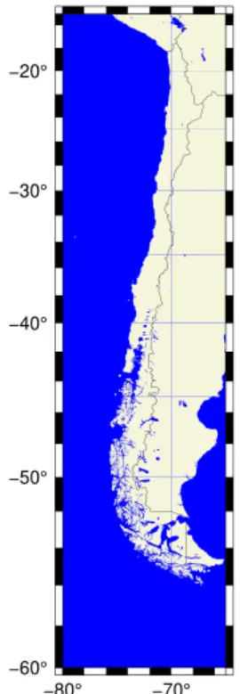
Because the two‐character ISO country code can be used in specifying a region, we can easily make a map with a region that suits Chile using the CL country code. However, that would yield a tight bounding box, hence we round to the nearest multiple of 5° in longitude and latitude. The resulting script is
gmt begin Fig_3 png
gmt coast -RCL+r5 -JM15c+du -BWSne -B -Gbeige -Sblue -N1/1p gmt end show
where we have limited automatic annotations (‐B) to the westside and southside (‐BWSne), added national borders (‐N1), and painted ocean (‐S) and land (‐G) separately. Because height will be much longer than width, we indicate that the map dimension (15c) sets the maximum dimension (+du). The resulting PNG illustration is shown in Figure 3. Atfirst sight, these three lines look like a step backward. In classic mode, such maps could be made with one line since there are no begin and end calls. For longer plot sequences, the benefits of modern mode simplicity outweigh the added work of starting and ending with begin and end.
6.2. Shaded DEM of Madagascar
To demonstrate the use of the remotefile mechanism we will make a relief image for Madagascar, including a color table. Our illustration (Figure 4) is made via the script
gmt begin Fig_4 png,pdf
gmt grdimage @earth_relief_01m -RMG+r2 -I+d gmt coast -Wthin -BWSne -B
gmt inset begin -DjTL+w3.5c+o0.2c -M0
gmt coast -Rg -JG47/-20/? -Ggray -Swhite -EMG+gred -Bg30 gmt inset end
gmt colorbar -DJTC -Ba -By+lkm -C+Uk gmt end show
Figure 3. Example of a modern mode plot of Chile, using the country code CL to set the plot region rounded to the nearest 5°.
which produces both a PNG and a PDF plot. There are several features to notice here, some of which contrast with how a similar plot would be made in classic mode. First, we select the 1 arc min remote DEM [which is the ETOPO1 data; Amante & Eakins, 2008] and request the nearest 2° bounding box for Madagascar. We implicitly select the geocolor table which will be scaled to fit the range of the grid inside the region. This scaled CPT is saved as a session current CPT and is available to subsequent modules that do not specify a CPT name, such as our colorbar command. Next, we compute artificial shading from that data grid with default settings for angle and intensity (‐I+d). We then draw the coastline and default map boundary (‐B), then begin a map inset to place a globe showing the location of Madagascar (the width of “?” means we wish to fit the plot in the space provided by the inset automatically), then end inset mode, place a colorbar cen-tered on top (‐DJTC), scaled to km (+Uk) and annotated accordingly, before we end the session.
6.3. Four Pacific Island DEMs
Next, we show a more complicated example using the new module sub-plot. We desire to show four Pacific island DEM images using the 1 arc sec SRTM data from NASA. Our script, resulting in the PDF in Figure 5, is gmt begin Fig_5
gmt set MAP_ANNOT_OBLIQUE 34 FORMAT_GEO_MAP ddd:mmF gmt makecpt -Cterra -T-3000/1500
gmt subplot begin 2x2 -M0.1c -Fs8c -BWSne -A+gwhite+p0.5p gmt subplot set 0,0
gmt grdimage @earth_relief_01s -R-30/30/-30/30+uk -JA159:32W/22:03N/? echo 159:29:55W 22:04:26N | gmt plot -Sc0.2c -Gred
gmt text -F+cTR+f12p,red+t"Mount Waialeale" -Dj0.2c gmt subplot set 0,1
gmt grdimage @earth_relief_01s -R-15/15/-15/15+uk -JA109:20W/27:07S/? gmt subplot set 1,0
gmt grdimage @earth_relief_01s -R-30/30/-30/30+uk -JA149:22W/17:43S/? gmt subplot set 1,1
gmt grdimage @earth_relief_01s -R-10/10/-10/10+uk -JA138:39W/10:29S/? gmt subplot end
gmt colorbar -Bx -By+lm -DJTC gmt end show
Inside this GMT modern mode session, we create a layout for a 2 × 2 subplot group where each subplot is 8 × 8 cm, with 0.1‐cm margins (‐M) between neighboring subplots and their annotations. We turn on automatic labeling of each frame (-A) using the default lower‐case letters in row‐order with a white, outlined box behind each label. Because each Pacific island (Kauai, Easter, Tahiti, and Fatu Hiva) has separate regions, each grdimage call needs to set its unique region and projection center. We use the azimuthal projection to set the center of each map and then use the‐R region to specify a square area in kilometers centered on that point. We scale the terra color table to cover the full range of the relief and use subplot set to move focus to the next subplot (row,col) in the sequence. After ending the subplot we place a colorbar centered on top of the 2 × 2 set of subplots using the outside top center justification (‐DJTC).
6.4. Animation of Earthquakes
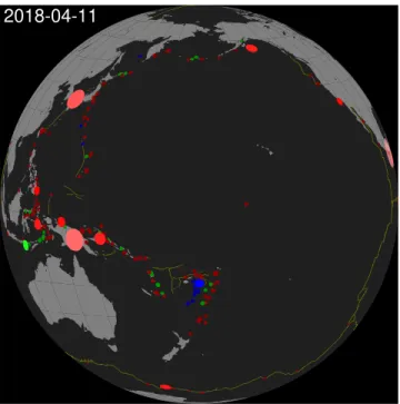
Finally, we demonstrate the ease with which to make animations by obtaining all magnitude 5 or above earthquake events for 2018 and creating a daily event movie with 365 frames. Our script, resulting both in a master PDF shown in Figure 6 as well as an MP4 movie available online (Wessel et al., 2019), consists
Figure 4. Example of a modern mode shaded relief image of Madagascar, using the country code MG to set the plot region rounded to the nearest 2° and placing a color bar on top and a location map inset in the upper left corner.
of two parts. First, we run a few commands to obtain the data via a URL query to USGS while setting the order of columns via convert ‐i and scaling the magnitudes by 50 to give suitable symbol sizes in kilometers, build a standard color table for use with earthquake depths, andfinally create a list of all dates in 2018 and assign a central longitude that linearly drifts from 160°E to 120°W during the year: # 1. Extract 2018 data from URL and prepare inputs and frame times
SITE="https://earthquake.usgs.gov/fdsnws/event/1/query.csv" TIME="starttime=2018-01-01%2000:00:00&endtime=2018-12-31%2000:00:00" MAG="minmagnitude=5" ORDER="orderby=time-asc" URL="${SITE}?${TIME}&${MAG}&${ORDER}" gmt begin
gmt convert $URL -i2,1,3,4+s50,0 -hi1 > q.txt
gmt makecpt -Cred,green,blue -T0,70,300,10000 -H > quakes.cpt
gmt math -T2018-01-01T/2018-12-31T/1–TIME_UNIT=d TNORM 40 MUL 200 ADD = times.txt gmt end
We then write a main frame script (quakes.sh) that uses the date column ($MOVIE_COL0) and longitude column ($MOVIE_COL1) from each row in times.txt to make a single coastline plot with mid‐ocean
Figure 5. Example of modern mode relief images of four Pacific islands (a. Kauai, b. Easter, c. Tahiti, d. Fatu Hiva) using the 1 × 1 arc sec SRTM grids from NASA, and adding a single, common color bar on top of the subplots. We also mark a location on Kauai and label that panel. SRTM = Shuttle Radar Topography Mission; NASA = National Aeronautics and Space Administration.
ridges shown, then overlays the events visible on that day: # 2. Write the main movie script (called quakes.sh): gmt begin
gmt coast -Rg -JG${MOVIE_COL1}/5/6i -G128 -S32 -X0 -Y0 -A500 gmt plot @ridge.txt -W0.5p,darkyellow
gmt events q.txt -SE- -Cquakes.cpt -TIME_UNIT=d -T${MOVIE_COL0} \ -Es+r2+d6 -Ms5+c0.5 -Mi1+c-0.6 -Mt+c0
gmt end
The events are scaled up in size when theyfirst occur and given a boost in color intensity, then decay to afinal smaller size and darker color a few days later. The movie module accepts the script and specifics of the movie dimension and format to build all frames in parallel and assemble the final MP4 movie automatically via the freely available FFmpeg tool (for more details on animations, please visit docs.generic‐mapping‐tools.org): # 3. Build the movie
gmt movie quakes.sh -C6ix6ix200 -Ttimes.txt -NFig_6 -Gblack -H2 -Lc0 \
-M100,pdf -Fmp4 –Z -FONT_TAG=20p,Helvetica,white –
FORMAT_CLOCK_MAP=-7. GMT Code and Documentation
The GMT source code has been managed using version control systems since the 1990s. However, we have gone through many different systems, from SCCS, CVS, subversion, and as of August 2018 we are using git. All GMT development can be accessed on our GitHub page (github.com/GenericMappingTools), and all aspects of GMT, with links to everything from source to docu-mentation on GitHub is found at this site (www.generic‐mapping‐tools.org). This site also maintains infor-mation on where and how to install GMT and how to contribute to the GMT project.
8. Future and In‐Progress Developments
Some aspects of GMT development are ongoing and notfinalized for the GMT 6 release. We are in the pro-cess of strengthening our map projection code by relying on PROJ.4, a generic coordinate transformation library that includes cartographic projections as well as geodetic transformations. Although GMT has always had its own projection code, the fact is that PROJ.4 has become the de facto projection library used by almost all free and Open Source projects. Because of this and the facts that its syntax is known to more people, that it supports more projection transformations and that in its recent evolution (PROJ.4 version 6) has seen the addition of the time dimension, we decided to start adopting PROJ.4 as the future projection library in GMT. This decision does not add any new dependency as we access it via its implementation through GDAL. The transition is not yet fully implemented as it requires deeper adaptations of the GMT machinery to plot the map frames, but it already works well for vector transforms. On the other hand, GMT 6 tries to maintain, to the extent possible, the compatibility with previous versions so we will accept both the classical ‐J GMT syntax as well as the typical PROJ.4 strings. For example, to do a Lambert Conformal Conic projec-tion of a geographic point, users can now run
echo 4.897 52.371 | \
gmt mapproject -J+proj=lcc+ellps=WGS84+units=m+lat_1=20n+lat_2=60n
Making projected images is also possible but so far, the available subset is restricted mostly to cylindrical pro-jections. Our second example plots a part of Africa using the Mercator projection:
Figure 6. Single frame (#50) of a 1‐year animation of daily frames showing the evolution of larger (> magnitude 5) earthquakes in the Pacific during 2018. On this particular day, a few large events happened near New Guinea and are still shown larger and brighter than earlier events. See Wessel et al. (2019) for the full MP4 movie.
gmt begin merc4
gmt coast -R-22/40/0/38 -J+proj=merc+ellps=WGS84+units=m+width=15c -W -B gmt end
Under the hood we are laying the groundwork for optional long‐format options in GMT. This means that instead of typing‐RUK ‐JM12c one can choose to write ‐‐region=UK ‐‐projection=mercator+width=12c. This enhancement will affect all options throughout GMT and will make scripting syntax much more read-able. It will also simplify the external interface parsers since they can pass such high‐level syntax directly to the GMT module.
We are also expecting to build a stronger coupling with GDAL for reading vector data. Currently, GMT can read shapefiles via a system call to ogr2ogr which produces a temporary GMT/OGR format file that GMT can read. However, like our bridge to GDAL for reading grids and images, we are interested in building a similar bridge for vector data.
Apart from modern mode modules, a few supplements have received new modules as well, and we have rearranged some supplements to betterfit their contents. The new geodesy supplement holds velo (moved from meca) and gpsgridder (moved from potential) and also has a new tool for computing solid earth tides (earthtide), while the seis supplement (formerly meca) has a new tool for plotting seismic waveforms (sac). Our website content is always changing, but having recently acquired the generic‐mapping‐tools.org domain we will serve the GMT community from this URL regardless of where GMT ultimately is hosted. Separate from the repository we will be offering GMT workshops both for users and developers in conjunction with major scientific meetings; these materials will also be available from our website.
References
Amante, C., & Eakins, B. W. (2008). ETOPO1 1 arc‐minute global relief model: Procedures, data sources and analysis. Rep., National Geophysical Data Center, Boulder, CO.
Caress, D. W., & Chayes, D. N. (1996). Improved processing of Hydrosweep DS multibeam data on the R/V/Maurice Ewing. Marine Geophysical Researches, 18(6), 631–650. https://doi.org/10.1007/BF00313878
Key, R. M., Kozyr, A., Sabine, C. L., Lee, K., Wanninkhof, R., Bullister, J. L., et al. (2004). A global ocean carbon climatology: Results from Global Data Analysis Project (GLODAP). Global Biogeochemical Cycles, 18, GB4031. https://doi.org/10.1029/2004GB002247 Luis, J. F., & Wessel, P. (2018). A Julia wrapper for the Generic Mapping Tools, Eos. Trans. AGU, Fall Meeting, (Abstract NS53A‐0563). McClusky, S., Balassanian, S., Barka, A., Demir, C., Ergintav, S., Georgiev, I., et al. (2000). Global Positioning System constraints on plate
kinematics and dynamics in the eastern Mediterranean and Caucasus. Journal of Geophysical Research, 105(B3), 5695–5719. https://doi. org/10.1029/1999JB900351
Müller, R. D., Seton, M., Zahirovic, S., Williams, S. E., Matthews, K. J., Wright, N. M., et al. (2016). Ocean basin evolution and global‐scale plate reorganization events since Pangea breakup. Annual Review of Earth and Planetary Sciences, 44(1), 107–138. https://doi.org/ 10.1146/annurev‐earth‐060115‐012211
Ritsema, J., Deuss, A., van Heijst, H. J., & Woodhouse, J. H. (2011). S40RTS: A degree‐40 shear‐velocity model for the mantle from new Rayleigh wave dispersion, teleseismic traveltime and normal‐mode splitting function measurements. Geophysical Journal International, 184(3), 1223–1236. https://doi.org/10.1111/j.1365‐246X.2010.04884.x
Sandwell, D. T., Mellors, R., Xiaopeng, T., Wei, M., & Wessel, P. (2011). Open radar interferometry software for mapping surface defor-mation. Eos, Transactions American Geophysical Union, 92(28), 234–235. https://doi.org/10.1029/2011EO280002
Smith, D. E., Zuber, M. T., Solomon, S. C., Phillips, R. J., Head, J. W., Garvin, J. B., et al. (1999). The global topography of Mars and implications for surface evolution. Science, 284(5419), 1495–1503. https://doi.org/10.1126/science.284.5419.1495
Steinberger, B., Sutherland, R., & O'Connell, R. J. (2004). Prediction of Emperor‐Hawaii seamount locations from a revised model of global plate motion and mantleflow. Nature, 430(6996), 167–173. https://doi.org/10.1038/nature02660
Uieda, L., & Wessel, P. (2017). A modern Python interface for the Generic Mapping Tools, Eos. Trans. AGU, Fall Meeting, (Abstract IN51B‐ 0018).
Wessel, P., Luis, J., Uieda, L., Scharroo, R., Wobbe, F., Smith, W. H. F., & Tian, D. (2019). GMT animation of magnitude 5+ seismicity in the Pacific Basin during 2018. figshare. Media. https://doi.org/10.6084/m9.figshare.8171339
Wessel, P., & Luis, J. F. (2017). The GMT/MATLAB toolbox. Geochemistry, Geophysics, Geosystems, 18, 811–823. https://doi.org/10.1002/ 2016GC006723
Wessel, P., Matthews, K. J., Müller, R. D., Mazzoni, A., Whittaker, J. M., Myhill, R., & Chandler, M. T. (2015). Semiautomatic fracture zone tracking. Geochemistry, Geophysics, Geosystems, 16, 2462–2472. https://doi.org/10.1002/2015GC005853
Wessel, P., & Smith, W. H. F. (1991). Free software helps map and display data. Eos, Transactions American Geophysical Union, 72(41), 441. https://doi.org/10.1029/90EO00319
Wessel, P., & Smith, W. H. F. (1995). New version of the Generic Mapping Tools released. Eos, Transactions American Geophysical Union, 76(33), 329. https://doi.org/10.1029/95EO00198
Wessel, P., & Smith, W. H. F. (1998). New, improved version of Generic Mapping Tools released. Eos, Transactions American Geophysical Union, 79(47), 579. https://doi.org/10.1029/98EO00426
Wessel, P., Smith, W. H. F., Scharroo, R., Luis, J. F., & Wobbe, F. (2013). Generic Mapping Tools: Improved version released. Eos, Transactions American Geophysical Union, 94(45), 409–410. https://doi.org/10.1002/2013EO450001
Acknowledgments
Development of the Generic Mapping Tools has been funded by the U.S. National Science Foundation since 1993 and has benefitted from the contributions of numerous scientists and enthusiasts. The contents of this manuscript are solely the work product of the authors and should not be construed as a statement of policy or position of NOAA or the U.S. Government. D. T. acknowledges support from the MSU Geological Sciences Endowment. Reviews by Graeme Eagles and Sabin Zahirovic greatly improved the paper. All software and support data are freely accessible and available from this site (www.generic‐mapping‐tools.org). This is SOEST contribution 10785.