Analysis of flow in branched stent-grafts for endovascular repair of the aortic arch

(1)

Chemical Engineering Integrated Masters’ Programme

Analysis of flow in branched stent-grafts for

endovascular repair of the aortic arch

Master Thesis

by

Ana Margarida Outeirinho Morgado

Developed within the Dissertation course

held in the

Biofluids and Transport Group of the Separation and Transport Laboratory

Department of Chemical Engineering

Imperial College London

Supervisor at Imperial College London: Professor Xiao Yun Xu Supervisor at FEUP: Professor João Moreira de Campos

Department of Chemical Engineering

(2)

(3)

(4)

(5)

Analysis of flow in branched stent-grafts for endovascular repair of the aortic arch

Acknowledgements

To Professor Xiao Yun Xu, for the opportunity.

To Professor João Campos, for the encouragement and the guidance. To Harkamaljot Kandail (Rocky), for the time, knowledge and patience.

To the 𝜒𝜇 group, for the friendly work environment.

To Ana Fumega and Ana Soares – “Dissertações ao ataque!” -, for all the knowledge, support and jokes exchanged.

(6)

Resumo

A interação entre o escoamento do sangue e as paredes das artérias promove, frequentemente, o aparecimento de doenças vasculares. No caso da crossa da aorta, o procedimento convencional para estas patologias é a cirurgia aberta, cuja taxa de mortalidade é de 7 a 17 %. Uma alternativa aliciante à cirurgia, por se tratar de um procedimento menos invasivo, é a reparação aórtica endovascular, que consiste na introdução de um stent-graft através de uma artéria de acesso.

Estudos experimentais e numéricos têm contribuído para uma maior e melhor compreensão das doenças cardiovasculares, assim como para o desenvolvimento de técnicas de diagnóstico e stent-grafts de melhor desempenho.

Este trabalho consistiu no estudo numérico do escoamento sanguíneo num modelo tridimensional simplificado da crossa da aorta, com os seus três vasos superiores, antes e depois da introdução de um stent-graft ramificado. Verificou-se que a introdução do stent- -graft aumenta a perfusão sanguínea através das três artérias superiores. Verificou-se, também, um aumento da tensão de corte nas paredes dos vasos, o que pode resultar em complicações pós-operatórias, e.g., migração do dispositivo.

Foi testada uma nova metodologia para estabelecer uma condição fronteira resistiva, que consiste na extensão do modelo da crossa da aorta por um tubo constritivo, o qual impõe sobre o domínio a resistência da restante vasculatura. As principais caraterísticas fisiológicas do escoamento foram estudadas, após as simulações. Verificou-se uma diminuição da magnitude do caudal, possivelmente devida ao facto da curvatura da crossa da aorta não ter sido considerada. Os valores da resistência mantiveram-se constantes em todas as simulações.

Três stent-grafts ramificados foram testados, de forma a avaliar o impacto do diâmetro dos seus ramos no desempenho dos dispositivos. Foi identificada uma zona de recirculação no bypass da subclávia esquerda através da carótida esquerda comum. Apesar do uso de um stent-graft personalizado garantir melhor desempenho, de modo a reduzir os atrasos e os custos associados à sua produção, deve ser dada preferência a dispositivos cujo diâmetro dos ramos seja ligeiramente superior ao das artérias.

Palavras Chave: reparação aórtica endovascular; crossa da aorta; stent-grafts

ramificados; dinâmica de fluidos computacional; condições fronteira resistivas.

(7)

Abstract

Vascular pathologies may arise from the interaction between blood flow and arteries walls. In the case of aortic arch diseases, the conventional open surgery procedure has a reported mortality rate of 7 – 17 %. Endovascular aortic repair, consisting in the introduction of a stent-graft through an access artery, constitutes an appealing alternative, being a less invasive procedure.

Haemodynamic studies performed both experimentally and numerically, have shed significant light over the characteristics of blood flow, leading to a better understanding of cardiovascular diseases and to the development of diagnosis tools and stent-grafts of improved performance.

In this work, numerical flow studies in simplified three-dimensional models of the aortic arch and three upper branches, before and after the introduction of an idealized branched stent-graft, were performed. The presence of the stent-grafts increases blood perfusion through the three supra-aortic vessels. Nevertheless, wall shear stress increases drastically after the introduction of the stent-graft, which may result in post-operative complications.

A new methodology for a resistance type outflow boundary condition, consisting in the attachment of a constriction tube to the outlets of the models, imposing the resistance of the downstream vasculature, was also tested. Using this methodology, the main physiological flow features are captured. A decrease in the flow rate magnitude is observed, possibly due to the absence of the arch’s curvature. The specific resistance held constant for all simulations.

Three branched stent-grafts were tested, in order to evaluate the impact of the diameter of the stent-graft’s branches in its hemodynamic performance. A persistent flow recirculation zone, FRZ, was identified in the bypass of the left subclavian artery through the left common carotid. Results suggested that, although the best haemodynamic performance would be achieved with customized branched stent-grafts, in order to minimize delays and costs, preference should be given to branches with slightly higher diameters than the ones of the vessels as these yield smaller FRZ.

Key-words: endovascular aortic repair; aortic arch; branched stent-graft;

(8)

(9)

Statement

I hereby declare that this is an original work and that all non-original contributions needed to its completion were dully referenced with the respective source clearly identified.

(10)

i

List of Figures

Figure 1 – The heart and its main vessels, with focus on the ascending aorta, the aortic arch, the brachiocephalic trunk or innominate artery, IA, the left common carotid, LCCA, and the left subclavian artery, LSCA. ... 6 Figure 2 - Anatomical landing zone map [13]. ... 7 Figure 3 – (A) Schematic representation of a aortic arch branched stent-graft with a branch for the innominate artery and occlusion of both the left common carotid and left subclavian arteries [16]. (B) Precurved fenestrated stent-graft for the aortic arch with fenestration for the three supra-aortic vessels [18]. ... 8 Figure 4 – Schematic drawing of the stent-graft prototype suggested by Finlay et al. [5]. A to E2:

geometric parameters based on frequency measurements of the aortic arch mapping. ... 9 Figure 5 – Stability diagram showing in vivo disturbed and undisturbed flow data [34]. ... 13 Figure 6 – Straight vessel with a rigid contraction tube [40]. ... 15 Figure 7 – Fluid domain. An artificially model of the aortic arch was selected as the fluid domain, ΩF. The idealized geometry was reconstructed with the physiological dimensions reported by Finlay et al. [5]. ... 17 Figure 8 – Modified geometries for the fluid domain, ΩF, including a branched stent-graft consisting of a main body and two tunnel stent-grafts for the innominate, IA, and the left common carotid, LCCA, arteries. (A) stent-graft 1; (B) stent-graft 2; (C) stent-graft 3. ... 18 Figure 9 – Rigid constriction tube representing the resistance type outflow boundary model. ... 20 Figure 10 – Volumetric flow rate waveform at the ascending thoracic aorta. The flow waveform was extracted from Xiao [39], and corresponds to patient data acquired via Phase-Contrast MRI of a healthy 28 year-old male subject. ... 21 Figure 11 – Volumetric flow rate waveform at the innominate artery, IA. The flow waveform was extracted from Xiao [39], and corresponds to patient data acquired via Phase-Contrast MRI of a healthy 28 year-old male subject. ... 21 Figure 12 - Volumetric flow rate waveform at the left common carotid artery, LCCA. The flow waveform was extracted from Xiao [39], and corresponds to patient data acquired via Phase-Contrast MRI of a healthy 28 year-old male subject. ... 21 Figure 13 - Volumetric flow rate waveform at the left subclavian artery, LSCA. The flow waveform was extracted from Xiao [39], and corresponds to patient data acquired via Phase-Contrast MRI of a healthy 28 year-old male subject. ... 22 Figure 14 – Schematic of the computational model adopted in this work in order to obtain the boundary conditions for the calibration of the constriction tubes. At the inlet and outlets of the model, the boundary conditions prescribed are represented. ... 22

(13)

iv

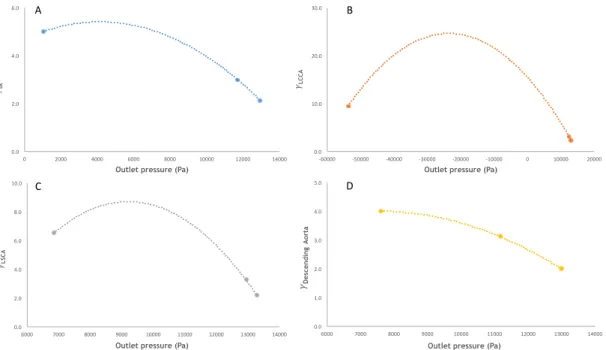
Figure 15 – Experimental relationship between the ratio of the outlet and inlet diameters, γi, and the outlet pressure for the constriction tubes for: (A) innominate artery, (B) left common carotid artery, (C) left subclavian artery, and (D) descending aorta. A second order polynomial trend line (dashed line) was used to establish the relationship between both variables. ... 23 Figure 16 – Schematic of the fully defined CFD model, ΩF, final, for all geometries: (A) the aortic arch model, and the aortic arch model including the branched stent-graft: (B) stent-graft 1, (C) stent- -graft 2, and (D) stent-graft 3.The black boxes highlight the constriction tubes. ... 24 Figure 17 – Stability diagram [34]. Representing the peak systole Reynolds number, Re, against the Womersley parameter, α, determined at the inlet (intersection of the red horizontal and vertical lines) yields a point in the laminar flow region. ... 27 Figure 18 – Flow rate waveforms prescribe in the calibration case from patient PC-MRI data (on the left) and those obtained in the reference case (on the right), for the three supra-aortic vessels. Results are presented over one cardiac cycle (0.76 s). ... 30 Figure 19 – Blood inflow split into the four outlets of the aortic arch model for the calibration and reference cases. ... 30 Figure 20 - Mean volumetric flow rate at the four outlets of the aortic arch model for the calibration and reference cases. ... 31 Figure 21 - Pressure waveforms at the four outlets of the aortic arch model, for the calibration and reference cases. Results are presented over a cardiac cycle (0.76 s). ... 31 Figure 22 – Flow rate waveforms at the four outlets of the aortic arch model, for a uniform and for a Womersley velocity profiles at the inlet (reference case). Results are presented over a cardiac cycle (0.76 s). ... 32 Figure 23 - Mean volumetric flow rate at the four outlets of the aortic arch model, for a uniform velocity profile and for a Womersley velocity profile at the inlet (reference case). ... 33 Figure 24 – Blood inflow split into the four outlets of the aortic arch model, for a uniform velocity profile and for a Womersley velocity profile at the inlet (reference case). ... 33 Figure 25 – Specific resistance for all outlets of the aortic arch model, for a uniform velocity profile and for a Womersley velocity profile at the inlet (reference case). ... 34 Figure 26 - Flow rate waveforms at the four outlets of the aortic arch models for the reference case and for the three geometries including a branched stent-graft: (A) stent-graft 1, (B) stent -graft 2, (C) stent-graft 3. ... 34 Figure 27 - Blood inflow split into the four outlets of the aortic arch models for the reference case and for the three geometries including a branched stent-graft: (A) stent-graft 1, (B) stent-graft 2, (C) stent-graft 3. ... 35

(14)

v

Figure 28 – Mean volumetric flow rate at the four outlets of the aortic arch models for the reference case and for the three geometries including a branched stent-graft: (A) stent-graft 1, (B) stent- -graft 2, (C) stent-graft 3. ... 35 Figure 29 - Specific resistance for all outlets of the aortic arch models for the reference case and for the three geometries including a branched stent-graft: (A) stent-graft 1, (B) stent-graft 2, (C) stent- -graft 3. ... 36 Figure 30 - Time-averaged wall shear stress, TAWSS, contours for the models of the aortic arch (A) without stent-graft, and including the branched stent-graft: (B) stent-graft 1, (C) stent-graft 2, (D) stent-graft 3. The arrows mark flow recirculation zones found in the bypass of the LSCA through the LCCA, which are regions of low TAWSS. ... 37 Figure 31 – Time-points over the cardiac cycle. ... 37 Figure 32 - Velocity streamlines during peak systole (t = 0.11 s) observed in the models of the aortic arch (A) without stent-graft, and including the branched stent-graft: (B) stent-graft 1, (C) stent- -graft 2, (D) stent-graft 3. ... 38 Figure 33 – Velocity streamlines during mid-deceleration time point (t = 0.21 s) observed in the models of the aortic arch (A) without stent-graft, and including the branched stent-graft: (B) stent- -graft 1, (C) stent-graft 2, (D) stent-graft 3. ... 38 Figure 34 - Velocity vectors highlighting the flow recirculation zones, FRZ, found in the models of the aortic arch (A) without stent-graft, and including the branched stent-graft: (B) stent-graft 1, (C) stent-graft 2, (D) stent-graft 3, at t = 0.21 s. ... 39 Figure 35 – Velocity vectors highlighting the separation and reattachment points of the flow recirculation zone, FRZ, at t = 0.21 s, in the bypass region of the three geometries including a branched stent-graft: (A) stent-graft 1, (B) stent-graft 2, (C) stent-graft 3. ... 40 Figure 36 – Lengths of the flow recirculation zone, FRZ, found in the bypass of the LSCA through the LCCA in the geometries including a branched graft: (A) graft 1, (B) graft 2, (C) stent--graft 3. ... 40

(15)

vi

List of Tables

Table A. 1 - Dimension of the geometric parameters used to describe the fluid domain. Models of the aortic arch including stent-graft: (A) stent-graft 1, (B) stent-graft 2, (C) stent-graft 3. ... 51 Table A. 2 - Mesh statistics for all geometries: (A) the aortic arch model without stent-graft, and the models including the branched stent-graft: (B) stent-graft 1, (C) stent-graft 2, (D) stent-graft 3. ... 52

(16)

vii

Notation and Glossary

𝑎 Radius m

𝐶 Compliance m3_.Pa-1

𝑑 Diameter m

𝐷_! Inlet diameter of the constriction tube m

𝐷! Outlet diameter of the constriction tube m

𝐾 Impedance Ω

𝐿_! Length of the largest section of the constriction tube m 𝐿! Length of the narrowest section of the constriction tube m

𝑝 Pressure Pa

𝑝 Mean pressure Pa

𝑄 Volumetric flow rate m3_.s

𝑄 Mean volumetric flow rate m3_.s

𝑄 Volumetric flow rate at peak systole m3_.s

𝑅 Resistance kg.m-4_.s-1

𝑅! Proximal resistance kg.m-4.s-1

𝑅! Distal resistance kg.m-4.s-1

Re Reynolds number

Re Reynolds number at peak systole

𝑆 Cross-sectional area m2

𝑡 Time s

𝑢 Velocity m.s-1

𝑢 Mean velocity m.s-1

𝑍 Proximal landing zone of the stent-graft

Greek Letters

α Womersley parameter

𝛾 Ratio between diameters

Γ Boundary

𝜇 Dynamic viscosity Pa.s

𝜌 Density kg.m3

𝜏 Wall shear stress Pa

Τ Period s 𝜐 Kinematic viscosity m2_.s-1 𝜔 Cardiac frequency s-1 Ω Domain Indexes 𝑐 Critical value 𝐹 Fluid

𝑖 Outlet of the model

𝑖𝑛𝑙𝑒𝑡 Value at the inlet

𝑛 Number of the landing zone of the stent-graft 𝑡 Value at the downstream vasculature

(17)

viii

List of Acronyms

3D Three-dimensional

3-EWM 3-Element Windkessel Model CFD Computational Fluid Dynamics

CT Computed Tomography

EVAR Endovascular Aortic Repair FEM Finite Element Method FRZ Flow Recirculation Zone(s) FSI Fluid-Structure Interaction FVM Finite Volume Method

IA Innominate Artery

LCCA Left Common Carotid Artery LSCA Left Subclavian Artery MRI Magnetic Resonance Imaging

PC-MRI Phase-Contrast Magnetic Resonance Imaging TAWSS Time-Averaged Wall Shear Stress

WHO World Health Organization WSS Wall Shear Stress

(18)

Introduction 1

1 Introduction

1.1 Motivation

As a response to the interaction between blood flow and arteries walls, blood vessels are able to remodel themselves over time, responding to the haemodynamic stresses they are facing. Vascular pathologies may appear as a biological response to the fluid mechanical environment.

According to the World Health Organization, WHO, cardiovascular diseases are the number one cause of death in the world, having caused 17.5 million deaths, in 2012 [1]. The most common pathologies of the aortic arch include aneurysm and dissection caused by the over time weakening of the aortic wall [2]. These vascular pathologies are associated with high risk of vessel’s rupture, underlying the need for emergency surgery in such cases.

The conventional procedure for aortic arch repair is open surgery, which has a reported 7 – 17 % mortality rate [3]. In the last decade, endovascular aortic repair, EVAR, has appeared as a successful less invasive surgical procedure, consisting in the introduction of a stent-graft through an exposed access artery. The device is conducted to the desired landing site, where it is fixated, excluding the aneurysm sac or the dissection’s false lumen from the mainstream blood circulation. Although EVAR for the descending aorta has acceptable rates of mid-term mortality and morbidity, EVAR for the aortic arch is still in development, owning to the challenges that this anatomical location represents.

The site’s complex geometry, with extensive curvature and the presence of the three supra-aortic vessels (the brachiocephalic trunk or innominate artery, the left common carotid artery and the left subclavian artery), makes it hard to obtain a landing zone of sufficient length for the stent-graft implementation. The particular haemodynamic of this anatomical region, due to both its angulated morphology and proximity to the heart, must be carefully studied in order to accurately access the device performance.

Although there are several options when choosing a stent-graft for aortic arch EVAR, in this work branched stent-grafts were selected. Branched stent-grafts consist of a main body stent-graft with fixed branches of specific dimensions that can be oriented into the vessels of the aortic arch, making them adaptable to a wide variety of anatomical geometries. The use of this type of devices is usually associated with hybrid repair, combining aortic arch bypass with stent-grafting, to ensure landing zones of sufficient length and prevent migration of the device. The use of off-the-shelf branched stent-grafts is a particularly appealing option since

(19)

Introduction 2

their use preclude delays associated with customization of the device, allowing to reduce costs and ensuring democratization of the EVAR technique.

Blood flow analysis is of major importance when addressing vascular pathologies. Several studies on the dependence of the development of vascular diseases on flow structure have suggested that different types of shear stresses can induce different responses in the endothelial cells that constitute de inner part of the arteries walls [2, 4]. Those results suggest the possibility for a correlation between the development of this lesions and the fluid mechanical environment to which the vessels are subjected. Studies on blood flow have shed significant light over its characteristics, leading to a better understanding of cardiovascular diseases and to the development of diagnosis tools and stent-grafts of improved performance.

Haemodynamic studies have been performed experimentally using both in vitro and in vivo experimental methods. In recent years, the development of Computational Fluid Dynamics, CFD, enabled the analysis of patient-specific haemodynamic through three- -dimensional numerical simulations.

1.2 Research question

In this work, numerical flow studies in simplified three-dimensional models of the aortic arch, with its three upper branches, before and after the introduction of an idealized branched stent-graft are performed.

The pre-operative geometry is based on the surgically relevant aortic arch mapping reported by Finlay et al., in 2012 [5]. The idealized branched stent-graft is also based on the prototype suggested by Finlay’s group [5]. As it is constructed based on the most frequent dimensions for the aortic arch, this hypothetical off-the-shell prototype stent-graft is expected to obviate the need for customization in 60 to 75 % of the cases, democratizing the use of this technique. Such results will allow to overcome one of the main disadvantages of the EVAR procedure: the delay on the device’s production along with the high costs associated with its customization [4].

In this work, a new and easy to implement methodology for a resistance type outflow boundary condition is also tested. This methodology consists in the attachment of a constriction tube to the outlets of the model, imposing the resistance of the downstream vasculature.

(20)

Introduction 3

1.3 Objectives

It is the aim of this work to analyse the blood flow in simplified three-dimensional models of the aortic arch, with its three upper branches, before and after the introduction of an idealized branched stent-graft, using CFD software. Along with the blood flow analysis, a new and easy to implement methodology for a resistance type outflow boundary condition is studied. The optimisation of the stent-graft design for the best haemodynamic performance is also assessed.

1.4 Thesis layout

This thesis begins with this introductory chapter, where a general perspective of the motivation and research questions underlying this work are presented.

Chapter 2 provides more detailed information on the aortic arch, the aortic arch pathologies and repair procedures for these diseases, highlighting the advantages associated with endovascular procedures using branched stent-grafts. An introduction to the use of Computational Fluid Dynamics in blood flow analysis, together with a review of the literature existing on this subject can also be found in this section.

The methodology employed in this work is presented in Chapter 3, where the construction of the models, as well as the mathematical and numerical flow modelling, from pre- to post-processing, are described.

In Chapter 4, the results from the numerical simulations are presented, followed by their discussion, dividing the work in two parts: the evaluation of the resistance type outflow boundary condition and the analysis of blood flow in the branched stent-grafts.

In the final chapter, the main conclusions, along with comments on the limitations of this work and suggestions for future ones are presented.

(21)

(22)

State-of-the-Art 5

2 State-of-the-Art

2.1 The aortic arch

The aorta is the main trunk of the vascular system, conveying oxygenated blood to the tissues of the body. It begins at the upper part of the left ventricle, with a diameter of approximately 3 cm, passing upwards and to the right for about 5 cm, arching backwards and to the left, over the root of the left lung, then descending within the thorax, and entering the abdominal cavity, presenting a diameter of about 1.75 cm [6]. It is usual to divide the aorta in three sections: the ascending, the arch, and descending, which is differentiated in the thoracic and the abdominal parts [6]. The focus of this work is on the aortic arch.

The ascending aorta is about 5 cm long, beginning at the base of the left ventricle [6]. As the ascending aorta continues into the aortic arch, the calibre of the vessels is slightly increased, due to a bulging of its right wall, causing a dilatation named the bulb of the aorta [6]. On transverse section at this level, the vessel presents an approximately oval outline.

The aortic arch begins at the level of the upper border of the second right sternocostal articulation, and runs first upwards, then backwards and to the left side of the trachea, passing downwards on the left side of the body, continuing into the descending aorta [6]. The arch has two curvatures, one with its convexity upward, the other forward and to the left.

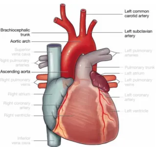
Three vessels arise from the upper part of the arch, supplying blood to the brain and upper parts of the body: the brachiocephalic trunk (innominate artery), the left common carotid artery and the left subclavian artery [6, 7]. A schematic representation of the heart with its main vessels, giving specific focus on the aortic arch and on the three supra-aortic vessels is shown in Figure 1.

The brachiocephalic trunk or innominate artery, IA, is the largest of the three supra- -aortic vessels, with a length of 4 - 5 cm [6]. It arises from the convexity of the arch, and divides itself into the right common carotid and right subclavian arteries at the level of the upper border of the right sternoclavicular [6]. The principal arteries of the head and neck are the two common carotids. The left common carotid artery, LCCA, springs from the higher part of the aortic arch, behind and to the left of the IA, ascending to the level of the left sternoclavicular joint [6]. Behind it is related to the left subclavian artery, LSCA, ascending to the root of the neck and then arching laterally [6].

(23)

Figure 1 – The heart and its main vessels, with focus on the ascending aorta, the aortic arch, the brachiocephalic trunk or innominate artery, IA, the left common carotid, LCCA, and the left

subclavian artery, LSCA.

As a response to the interaction between the blood flow and their walls, the arteries are able to remodel themselves over time, alteration that can lead to the development of diseases. The walls of the aorta consist of three thick, muscular and elastic layers: the tunica intima, tunica media and tunica adventitia, counting from the lumen [7]. Wall shear stress, WSS, has been reported as being intrinsically related to aortic pathologies [2, 7-9], with the biggest impact being seen on the intima layer that incorporates the endothelial cells in direct contact with blood.

Common diseases of the aortic arch include aneurysm and dissection. Aneurysms are local enlargements of the artery, causing thinning of the vessels wall [9]. The development of an aneurysm increases the risk of aortic dissection, which consists in the tear of the intima layer, causing blood to pass through this separation of layers of the aortic wall, producing a false lumen [10, 11]. The weakening of the aortic wall that occurs in this pathologies can lead to aortic rupture within minutes or hours of the acute event, after which the patient’s risk of death increases 1 % per hour [12]. This imminent risk of rupture underlies the necessity of emergency surgery in aortic arch pathologies.

2.2 Endovascular repair of the aortic arch

The conventional procedure for the treatment of aortic arch pathologies is open surgery, which has a reported 7 - 17 % mortality rate and a 4 – 12 % neurological injury rate [3]. In the last decade, endovascular aortic repair, EVAR, appeared as a successful less invasive technique, consisting in the introduction of a stent-graft through an exposed access

(24)

artery, excluding the aneurysm sac or the dissection’s false lumen from the mainstream blood circulation. Although EVAR has acceptable rates of mid-term mortality for the descending aorta, EVAR for the aortic arch is less developed due to the challenges that this anatomical site represents [3, 13].

A particularly important feature of EVAR techniques using stent-graft is the need for a sufficiently long length of healthy aorta to use as the landing site, with, according to Ishimaru et al. [13], at least 15 mm from an arch vessel to the margin of aneurysm being required. However, in the aortic arch, the curvature and proximity of the entrance of the three vessels (IA, LCCA and LSCA) makes it difficult to obtain a landing zone with sufficient length to ensure firm fixation of the device [13].

The need to maintain blood flow to the brain and upper extremities of the body must be assessed as well, and several alternatives to assure cerebral perfusion have been reported. Some of the currently available options for EVAR of the aortic arch include (I) hybrid repair – combining aortic arch bypass with stent-grafting, and the use of (II) branched or (III) fenestrated stent-grafts.

When considering EVAR that requires aortic arch landing, techniques are usually classified according to the proximal landing zone, 𝑍, as proposed by Balm et al.: 𝑍3 if landing is possible in the distal arch, 𝑍2 if only LSCA is occluded by the stent-graft, 𝑍1 if both LCCA and LSCA are occluded and 𝑍0 if all three supra-aortic vessels are occluded (Figure 2) [14].

Figure 2 - Anatomical landing zone map [13].

With aortic arch repair, at least 𝑍2 landing is usually required, thus a bypass of the LSCA through the LCCA to ensure blood perfusion to the upper left side of the body is

(25)

essential, since the entrance of the LSCA in the aortic arch will be occluded [14]. Hybrid procedures combine the use of endovascular devices with bypass for revascularization of the cervical vessels occluded by the stent-graft, being a less invasive technique than open surgery, with promising early- and long-term results. In 2014, Shirakawa et al. [3] reported on the efficacy and short-term results of combined supra-aortic bypass and stent-graft into the ascending aorta for 40 high-risk patients with aortic arch pathologies. The group achieved a 3 % 30-day mortality rate and 0 % incidence of stroke occurrence, with 85 % of the patients being able to recover at home and return to independent lifestyles. Hybrid techniques are an appealing option for high-risk patients since the aortic arch bypass creates a proximal landing zone of adequate length for stent-graft deployment, preventing migration of the device.

EVAR for the aortic arch using branched stent-graft (Figure 3.A) was first reported by Inoue et al., in 1997 [15], and later by Chuter and colleagues [16]. This type of devices consists of a main body stent-graft with fixed branches of specific dimensions that can be oriented into the arch’s vessels. Such characteristic makes them adaptable to a wide variety of anatomical geometries.

On their turn, fenestrated stent-grafts (Figure 3.B) are customized devices in which fenestrations in the main body are aligned with the entrance of the supra-aortic vessels and secured to these by covered stents [17]. These fenestrations will house supplemental stent- -grafts that protrude into the supra-aortic vessels. As these devices need to be tailor-made to ensure that the fenestrations are correctly aligned with the vessels, they require several weeks in the manufacturing, rendering their use expensive and unsuitable for urgent cases [4, 5, 17]. As mentioned by Finlay et al. [5], off-the-shelf branched stent-grafts would preclude this delay and reduce costs, ensuring democratization of the EVAR technique.

Figure 3 – (A) Schematic representation of a aortic arch branched stent-graft with a branch for the innominate artery and occlusion of both the left common carotid and left subclavian arteries [16]. (B) Precurved fenestrated stent-graft for the aortic arch with fenestration for the three supra-aortic

(26)

In 2012, Finlay et al. [5], performed a surgically relevant aortic arch mapping using Computed Tomography, CT, scans. After mapping the aortic arch diameters, branch orientations and centre line distances, the group proposed a prototype for a standard off-the--shelf stent-graft (Figure 4) that would obviate the need for customization in 60 to 75 % of cases, since its dimensions were based on the most common values obtained in CT scans [5].

Figure 4 – Schematic drawing of the stent-graft prototype suggested by Finlay et al. [5]. A to E2:

geometric parameters based on frequency measurements of the aortic arch mapping.

2.3 Modelling blood flow using Computational Fluid Dynamics

Studies on blood flow have shed significant light over its haemodynamic characteristics, leading to a better understanding of cardiovascular diseases and to the development of diagnosis tools and stent-grafts of improved performance.

Haemodynamic studies have been performed experimentally since the 1960s using both in vitro and in vivo methods. In recent years, the development of Computational Fluid Dynamics, CFD, enabled the analysis of patient-specific haemodynamic through three- -dimensional, 3D, numerical simulations. CFD simulations allow for the quantification of variables not measurable in vivo, and are appropriate for a combination with image-based measurements data [19]. CFD studies can be divided into four steps: problem identification, pre-processing, solving and post-processing.

2.3.1 Problem Identification

Vascular lesions tend to develop in regions of complex vessel geometry, as it is the case of the aortic arch. Several authors have used CFD simulations to study the

(27)

haemodynamic in this particular region [19-23]. In fact, the curvature and non-planarity of the arch, together with the tapering of the aorta from its ascending to descending portions, have been reported as responsible for the helical patterns and flow recirculations observed there [19-23].

2.3.2 Pre-processing

The first step when carrying out blood flow simulations is to define the geometry of the region under study. Simulations can be performed in idealized or image-based patient- -specified geometries.

Experimental and computational studies, conducted using both straight and curved tubes, provided a keen understanding on the influence of the arch’s curvature, documenting the skewness of the velocity profiles and the appearance of secondary flow patterns. They have also provided knowledge on the influence of the non-Newtonian blood behaviour, fluid- -structure interaction, mass transport phenomena, Reynolds and Dean dimensionless numbers, and Womersley parameter [19-21, 23]. The most common simplifications considered, when using idealized geometries for the aortic arch, include the assumption of circular cross-section of constant diameter, and negligence of both the curvature of the arch and the presence of the supra-aortic vessels.

Providing a realistic description of the anatomical region, image-based patient-specific geometries acquired via Magnetic Resonance Imaging, MRI, or CT scans have gain great popularity in the recent years. Using CT scans, high spatial resolution X-ray images are obtained with thin slice thickness and high contrast, allowing the distinct observation of different body parts through contrast adjustment. Nevertheless, CT scans are related to a certain degree of radiation, while the MRI technique, where contrast is achieved by exploiting differences in the magnetic spin relaxation properties of the body tissues and fluids using blood as the contrast agent, is thought to be benign [7, 19]. After image acquisition, it is necessary to reconstruct the geometry as a 3D model.

Once the 3D model is created, it is discretized into a mesh of finite number of smaller sub–domains over which the governing equations are solved. The smaller the number and distribution of these elements, the more accurate the simulation will be, at expense of computational costs, being essential the optimization of the ratio between solution accuracy and computational resources employed.

Meshes can be structured (hexahedral) or unstructured (tetrahedral). For the curved tubes or idealized geometries aforementioned, structured meshing has been usually used, since it can be easily automated, while unstructured meshes produced by commercial

(28)

meshing software are commonly used in patient-specific simulations due to its potential of effortless grid generation over complex geometries [19]. In the later approach, distributions of tetrahedral, prismatic and pyramid elements are generated using a variety of sophisticated algorithms requiring higher resolution to reach mesh independency. When the focus of the study is on wall shear stress, boundary layer mesh generation techniques with high resolution, i.e., higher mesh density near the artery wall, should be employed.

It is also essential to consider the accurate properties of the materials. Blood is a non--Newtonian fluid, since its viscosity decreases with the increase of the shear-rate, i.e., it is a shear-thinning fluid [7, 19]. Blood’s viscosity increases with the increase of the volume percentage of red blood cells and the decrease of body temperature [19]. The presence of red blood cells, measured in terms of their percentage, haematocrocit, gives some elasticity to the blood, which can be classified as a visco-elastic fluid. Nevertheless, the majority of the CFD studies assume blood as having a Newtonian behaviour, based on the premise that the mean shear-rate in the boundary layer exceeds 100 s-1, minimum value for which the viscosity is independent of the shear-rate [7]. Sustaining this assumption is the study by Fung et al. [24], reporting that blood viscosity has a milder impact on the shear forces acting in the vessels walls, compared to the effects of blood pressure and pressure waveforms.

The arteries are dynamic systems that adapt over time to the haemodynamic conditions to which they are subjected, in addition to expanding and relaxing throughout the cardiac cycle. The adaptation of the walls owes primarily to the long-term variations in the WSS, 𝜏!, sensed directly as a force onto the endothelial cells [2]. Equation 2.1 describes WSS

for a Newtonian fluid, where 𝑢 is the velocity, which is zero on the wall, 𝜇 the fluid’s dynamic viscosity, and 𝑎 the radius of the vessel. Blood pressure has also been reported as contributing for the dynamic response of the arteries, affecting primarily the cells on the tunica media layer [2].

𝜏!= − 𝜇

d𝑢

d𝑟 !!! (2.1)

Fluid-Structure Interaction, FSI, assigns the dynamic behaviour of the elastic walls as a response to the pulsatile blood flow and pressure. Modelling FSI is currently one of the major challenges in CFD haemodynamic simulations due to its dependence on blood flow and pressure, as well as on the tissues and organs outside the vessel, requiring extensive models of the arterial system as an all. Rigid wall assumption is commonly employed in CFD simulations, although FSI provide a more accurate description of the physiology of the site

(29)

under study. However, the latter requires complex numerical algorithms and patient-specific data, drastically increasing the need for computational resources.

In order to run CFD simulations and solve the governing equations it is essential to prescribe boundary conditions that match accurately clinical data.

Although the aorta is subjected to large deformations over time due to blood flow and pressures waveforms, and it is coupled with the surrounding organs and tissues, rigid, impermeable wall and no-slip conditions at the wall of the vessels are assumed in the majority of CFD studies [11, 19-29]. The effect of blood particles is also not considered as it is expected that such approximation would yield minor effects on the simulation results, according to Lam et al. [30].

In the human body, the majority of the studies assume laminar flow since, even in large arteries, the velocity has been reported to be low enough to yield relatively low Reynolds numbers [24, 26, 27]. Stein and Sabbah [31], in 1976, followed by Kilner et al. [32], in 1997, reported the flow through the aorta of a normal adult at rest as being laminar with possible disturbances, helical and disturbed flows patterns, in specific zones. The presence of abnormalities that change the widening of the blood vessel, e.g., atherosclerosis, aneurysms, dissections and stenosis, cause the flow inside the lumen to vary as well [7].

The Reynolds number, Re, given by Equation 2.2, where 𝑢 is the cross-sectional mean velocity of the fluid, 𝑑 the vessel’s diameter, 𝜌 the density of the fluid, 𝜇 the fluid’s dynamic viscosity and thus 𝜐 its kinematic viscosity, is a measure of the ratio between the inertial and viscous forces acting onto a fluid element [33].

Re = 𝑑!. 𝑢!. 𝜌 𝑑. 𝑢. 𝜇 = 𝑑. 𝑢. 𝜌 𝜇 = 𝑑. 𝑢 𝜐 (2.2)

For Re values smaller than the critical, Re!, the magnitude of the viscous forces

surpasses the one of the inertial forces, and the flow is said to be laminar, while a flow for which Re > Re_! is said to be turbulent. In the human aorta, the Re is approximately 4 000 and turbulent flow has been reported to be present when the peak Reynolds (Re at peak systole, Re) is between 5 000 and 6 000 [2, 19].

Kousera et al. [34], in their numerical study of aortic flow stability, presented a stability diagram, in Figure 5, showing in vivo disturbed and undisturbed flow data depending on the Re and the Womersley parameter.

(30)

Figure 5 – Stability diagram showing in vivo disturbed and undisturbed flow data [34].

The Womersley parameter, α, is a dimensionless frequency parameter governing the relationship between the unsteady and viscous forces acting onto to the fluid element. It is mathematically described by Equation 2.3, where 𝑎 is the characteristic dimension of the vessel, its radius, 𝜐 the kinematic viscosity and 𝜔 the cardiac frequency [7].

α = 𝑎 𝜔

𝜐 (2.3) For low α values, viscous forces dominate over unsteady ones, and velocity profile is parabolic with the centreline velocity oscillating in phase with the pressure gradient [2]. It is considered that for α > 10 the unsteady inertial forces predominate, and the velocity profile is almost flat due to a piston-like flow motion of the flow [2].

The most common inlet boundary condition in blood flow analyses consists in prescribing an idealized velocity profile (flat, parabolic or Womersley flow pattern) together with a pulsatile waveform. In 1955, Womersley reported data on the oscillatory motion of a viscous fluid in a thin-walled elastic tube, when subjected to a pressure gradient, proposing a mathematical solution for the blood flow rate in large arteries [35]. In this work, Womersley reported fare agreement when comparing the data with determinations made using high- -speed cinematography to study the motion through the translucent arterial wall [35]. Several in vivo studies using hot-film anemometry, such as those conducted by Seed and Wood [36], in 1971, and Nerem et al. [37], in 1972, have verified that the velocity profile is essentially flat in the beginning of the ascending aorta, then skews towards the inner wall in the aortic arch, with the development of a weak helical flow. The pulsatile waveform can be

(31)

obtained from patient-specific MRI, Phase-Contrast MRI, PC-MRI, or CT data, or extracted from literature, being the experimental data reported by Pedley [38] the most common reference [11, 19, 20, 29, 39].

Time-varying pressure waveforms are less frequently applied as inlet boundary condition since determination of the pressure using in vivo catheterization techniques are extremely invasive and may induce errors by disturbing the blood flow [19].

The intensity and magnitude of the pulsatile flow and pressure waveforms generated at the heart decrease towards the capillaries. Thus, outflow boundary conditions depending on the downstream vasculature have been the focus of several studies [19]. Being impossible to trace the complete vasculature in a simulation, the model must be truncated at some point, and the downstream system must be lumped in a way that allows for an exact description of the vasculature, ensuring realistic representation of the wave propagation.

The most common CFD outlet boundary conditions for large arteries include constant or pulsatile pressures, constant/zero traction, velocity profiles, pure resistance, 3-Element Windkessel, and Structure Tree models [19, 40]. Nevertheless, some of the aforementioned do not replicate accurately the system’s haemodynamic behaviour.

Since blood flow and pressure waveforms are coupled together - the pressure gradient along the arteries is the driving force of the blood flow - prescribing constant (zero) pressure at the outlet and pulsatile flow rate at the inlet seems to be a contradiction, even if the mean pressure difference between these boundaries is only a small fraction of the systolic- -diastolic pulse amplitude [19]. The popularity of this technique arises from the difficulty in obtaining experimental patient-specific data on pressure, as previously mentioned, although the constant pressure approach may only be valid at the capillary level [40].

Prescribing pure resistance, assuming that pressure, 𝑝, and flow, 𝑄, are directly proportional (𝑝 = 𝑅. 𝑄, where 𝑅 is the resistance), constrains 𝑝 and 𝑄 to be in phase and eliminates the effect of the truncated vasculature [40].

The 3-Element Windkessel Model, 3-EWM, is a lumped model relating 𝑃 and 𝑄 through a linear ordinary differential equation (Equation 2.4, where 𝑅! and 𝑅! are the proximal and

distal resistances, and 𝐶 the compliance), capturing the compliant and resistive effects of the vasculature, but falling short in capturing wave reflection throughout the vascular network [40]. d𝑝 d𝑡 = 𝑅! d𝑄 d𝑡 + 1 𝑅_!. 𝐶 𝑅!+ 𝑅! 𝑄 − 𝑝 (2.4)

(32)

The Structured Tree Model (impedance boundary condition) was developed by

Olufsen [41], in 2000, and modified by Vignon-Clementel et al. [25], in 2006. It relates 𝑝 and 𝑄 in the time domain through Equation 2.5, where 𝑘 is the inverse Fourier transform of the impedance in the frequency domain, 𝐾 (𝑥, 𝜔). Although the phase shift between 𝑝 and 𝑄 is considered, the periodicity assumption, given by the period, 𝛵, is not applicable for non- -periodic phenomena simulation [40].

𝑝 𝑥, 𝜔 = 1 𝑇 𝑘 𝑥, 𝑡 − 𝜉 . 𝑄 𝑥, 𝜉 d𝜉 !/! !!/! (2.5) In 2011, Pahlevan et al. [40] presented a new outflow model for FSI of blood flow in

cardiovascular systems. In the model, the computational domain is extended through an elastic tube connected to a rigid contraction, where user-defined geometrical and material properties allow the preservation of the desired resistance, compliance, and appropriate wave reflection of a truncated vasculature. The model, Figure 6, was applied to a 3D model of the aorta and the solutions correctly captured the physiological flow behaviour.

Figure 6 – Straight vessel with a rigid contraction tube [40].

For branched geometries, such as the one of the aortic arch, a widely used outlet boundary condition is to prescribe constant fractions of the inflow rate through each branch of the aorta [19, 27, 29]. This approach turns out to be unrealistic since the artery experiences considerable diameter variations throughout the cardiac cycle, as reported by van Prehn et al. [28], in 2007, and the assumption of constant flow through the branches states itself as inadequate. Although Pahlevan’s group [40] only presented results for single outlets, they claimed that multiple outlets can be incorporated into the model by applying the outflow boundary condition from Figure 6 to each individual outlet.

(33)

2.3.3 Solving

Blood flow in the aorta is typically sufficient for blood to be assumed as an incompressible, homogenous, Newtonian fluid with a time-dependent 3D flow. The governing principles of which can be described by the conservation laws of mass (continuity equation) and momentum, i.e., by the Navier-Stokes equations [24, 26, 27, 30].

The system of equations has an exact solution only for laminar flows of simple fluids. For more complex flows numerical methods implemented using CFD software are needed to solve the governing equations. Two of these methods are the finite element method, FEM, and the finite volume method, FVM.

To describe the variation of the unknown variables, the FEM makes use of approximate piecewise polynomial functions that are substituted into the governing equations. As the functions do not hold exactly during substitution, residuals are used to evaluate the errors. These errors must be minimized by multiplying them by a set of weighting function followed by integration [19]. This procedure yields a system of algebraic equations for the unknown variables.

The FVM uses an integral form of the governing equations directly into a finite number of sub-domains of smaller size – control volumes -, ensuring global conservation [19]. The terms of the integrated equation are then substituted by finite difference approximations yielding a system of algebraic equations that can be solved iteratively [19]. This methodology is valid for both structured and unstructured meshes. When using CFD software that employs FVM, attention must be taken when choosing the convergence criterion.

2.3.4 Post-processing

Once the governing equations are solved, i.e., the desired convergence criterion is reached, the simulation results can be visualized and must be analysed.

For the ascending aorta and aortic arch, WSS remains the parameter most commonly studied, and has been depicted by spatial maps or trends [19]. In the case of branched geometries, studies have showed that velocity iso-contours are ideal for visualizing or quantifying the regions of flow recirculation and of retrograde flow, common patterns in these anatomical sites [19].

The results from CFD simulations must be validated in order to determine the degree to which the model exactly represents the real case under study. Validation of CFD studies requires a combination of numerical results with experimental data, and is primarily done using in vitro models [19]. Few cases of validation with in vivo data have been reported [19].

(34)

Methodology 17

3 Methodology

3.1 Geometries

When performing CFD simulations, the first step is to select the fluid domain, Ω!, of

interest. As the focus of this work is on the aortic arch, this anatomical region was selected as Ω!, and artificially reconstructed with the physiological dimensions reported by

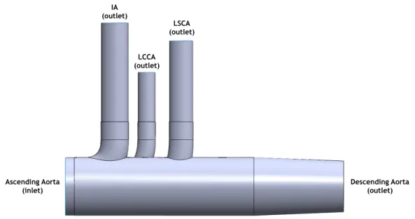
Finlay et al., in the group’s aortic arch mapping [5]. This idealized domain (Figure 7) encompasses part of the ascending aorta, the aortic arch with its three branches (innominate artery, IA, left common carotid artery, LCCA, and left subclavian artery, LSCA), and part of the descending aorta.

Figure 7 – Fluid domain. An artificially model of the aortic arch was selected as the fluid domain, 𝛺!.

The idealized geometry was reconstructed with the physiological dimensions reported by Finlay et al. [5].

Besides the geometry on Figure 7, CFD simulations were performed on three other modified geometries, which included a branched stent-graft consisting of a main body and two tunnel/branch stent-grafts for the IA and the LCCA. Such geometries were based on the prototype suggested by Finlay et al. [5], with the difference that, in the current work, occlusion of the LSCA and consequent bypass of this vessel through the LCCA, was considered. Such method was preferred since, for repair of aortic arch pathologies, at least 𝑍2 landing (Figure 2, in Chapter 2) is usually required, thus making necessary the bypass of the LSCA through the LCCA [14]. This hybrid technique has proven itself to be an appealing option for

Ascending Aorta (inlet) Descending Aorta (outlet) IA (outlet) LCCA (outlet) LSCA (outlet)

(35)

Methodology 18

high-risk patients since the occlusion of the vessel creates a proximal landing zone of adequate length for stent-graft deployment, preventing migration of the device.

As off-the-shelf branched stent-grafts are only manufactured in a small range of sizes, one of the aims of this work is to access the impact of the diameter of the tunnel stent-grafts for the supra-aortic vessels on the flow characteristics. This is the reason why three combinations for the diameter of the tunnel stent-grafts were tested:

- In the first geometry, the diameter of the tunnel stent-grafts matched the one of the vessels reported in the aortic arch mapping of Finlay et al. (15 mm for the IA, and 9.5 mm for the LCCA) – stent-graft 1;

- In the second (stent-graft 2) and third (stent-graft 3) geometries, the diameter of the tunnel stent-grafts was set equal to some of the most commonly manufactured diameters (8 mm and 10 mm, respectively for each geometry, for both IA and LCCA).

These new geometries are represented in Figure 8, where the difference in the diameters of the tunnel stent-grafts is made clear by the distance between their inlets, at the proximal (left) side of the models.

Figure 8 – Modified geometries for the fluid domain, 𝛺!, including a branched stent-graft consisting of a

main body and two tunnel stent-grafts for the innominate, IA, and the left common carotid, LCCA, arteries. (A) stent-graft 1; (B) stent-graft 2; (C) stent-graft 3.

Although the curvature and non-planarity of the arch have been reported to be responsible for helical and recirculating flow patterns observed in the anatomical region

A" B"

(36)

Methodology 19

under study [19-23], neglecting the curvature is expected not to have a significant impact on the results, particularly in a preliminary approach.

The outlet length of the three supra-aortic branches was extended by five times the respective diameter, in all geometries (Figures 7 and 8), to ensure fully developed flow at their outlet, as recommended by CFD software, ANSYS CFX 15.0 (ANSYS, Canonsburg, PA, USA) [34]. Also, a cylindrical extension of arbitrarily length (5 mm) was added to the inlet to provide developed flow at the entrance of the supra-aortic vessels [17].

The dimensions of the geometric parameters used to describe the geometries can be found in Table A.1, in the Appendix.

The 3D idealized geometries were constructed using commercially available software SolidWorks 2012 (Dessault Systemes, France).

3.2 Mathematical flow modelling

In all the simulations carried out in this work, blood was considered to be a Newtonian fluid, with a density, 𝜌, of 1 060 kg/m3_{and a constant dynamic viscosity, 𝜇, of 0.004 Pa.s [2,}

11], feasible assumptions for large arteries such as the aorta, as it is explained in Chapter 2. Effects of the blood particles were not considered since, according to Lam et al. [30], they would have a minor effect on the simulation results. Flow was assumed to be laminar, common assumption in the majority of the blood flow studies, and was modelled through the Navier-Stokes equations - continuity (Equation 3.1) and momentum (Equation 3.2) conservation equations, where 𝑢 represents the velocity, 𝑝 the pressure and 𝑡 the time.

∇. 𝑢 = 0 (3.1)

𝜌 𝜕𝑢

𝜕𝑡 + 𝑢. ∇. 𝑢 = −∇𝑝 + 𝜇∇!𝑢 (3.2)

The walls of the arteries and of the stent-graft were assumed to be solid, rigid, motionless and impermeable. For all simulations, a no-slip boundary condition was specified at the walls.

(37)

Methodology 20

3.3 Numerical flow modelling

Besides analysing blood flow in an idealized model of a branched stent-graft for EVAR of the aortic arch, a new, and easy to implement, methodology for a resistance type outflow boundary condition is also studied in this work. Resistance type outflow boundary conditions were implemented in all four outlets of the geometries tested, using the methodology described in the following section.

3.3.1 Resistance type outflow boundary condition

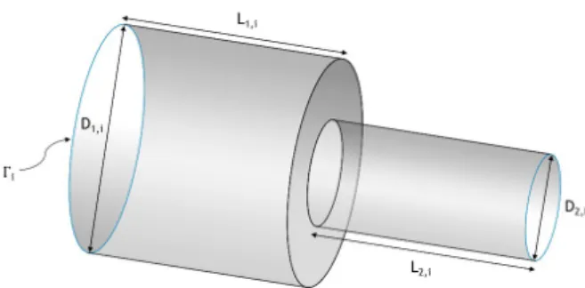
Resistance type boundary conditions were imposed at the outlet boundaries, Γ!, by

attaching a rigid constriction tube (Figure 9) at every outlet. These constriction tubes were calibrated so that they can accurately offer the resistance imposed by the downstream vasculature at every Γ!.

Figure 9 – Rigid constriction tube representing the resistance type outflow boundary model.

For the calibration of the constriction tubes, the first step was to determine the mean pressure values, 𝑝!, and volumetric flow rates, 𝑄!, at the four outlets of Ω! (𝑖 = IA, LCCA,

LSCA and descending aorta). This was done performing transient simulation on Ω! from

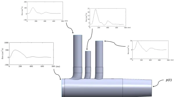
Figure 7, prescribing:

- At the inlet, a flat velocity profile combined with pulsatile flow rate waveform (Figure 10) extracted from PC-MRI data of a healthy 28 year-old male subject published by Nan Xiao [39];

- At the outlet of the three supra-aortic vessels, patient PC-MRI flow waveforms extracted from the same work (Figures 11 to 13);

- At the outlet of the descending aorta, a pressure waveform obtained by coupling the outlet with a 3-EWM, using an in-house Matlab R2015a (MathWorks, Natick, Massachusetts, USA) code. The parameters of the 3-EWM were obtained using the Nelder-Mead Simplex

(38)

Methodology 21

algorithm. Pressure was imposed to be in the physiological range, i.e., between the diastolic value of 80 mmHg and the systolic peak of 120 mmHg.

Figure 10 – Volumetric flow rate waveform at the ascending thoracic aorta. The flow waveform was extracted from Xiao [39], and corresponds to patient data acquired via Phase-Contrast MRI of a healthy

28 year-old male subject.

Figure 11 – Volumetric flow rate waveform at the innominate artery, IA. The flow waveform was extracted from Xiao [39], and corresponds to patient data acquired via Phase-Contrast MRI of a

healthy 28 year-old male subject.

Figure 12 - Volumetric flow rate waveform at the left common carotid artery, LCCA. The flow waveform was extracted from Xiao [39], and corresponds to patient data acquired via Phase-Contrast

(39)

Methodology 22

Figure 13 - Volumetric flow rate waveform at the left subclavian artery, LSCA. The flow waveform was extracted from Xiao [39], and corresponds to patient data acquired via Phase-Contrast MRI of a

healthy 28 year-old male subject.

Figure 14 shows a schematic representation of the boundary conditions prescribed in this calibration case.

Figure 14 – Schematic of the computational model adopted in this work in order to obtain the boundary conditions for the calibration of the constriction tubes. At the inlet and outlets of the

model, the boundary conditions prescribed are represented.

Four constriction tubes were constructed, one for each outlet of Ω!. These

constriction tubes constitute the outflow boundary models to be attached to the outlets of Ω!, similarly to method described by Pahlevan et al. [40].

(40)

Methodology 23

The main characteristic parameters required in order to fully define the constriction tubes are the ratio between the outlet and inlet diameters, 𝛾! = 𝐷!,! 𝐷!,!, and the lengths 𝐿!,!

and 𝐿!,!, along with the pressure at the outlet of the tubes, which will correspond to the one

of the downstream vasculature, 𝑝!,! (Figure 9). In order to represent accurately the pressure

at the capillaries, 𝑝!,! should be as close as possible to 0 Pa. To be attached to the outlets of

Ω_!, the inlet diameter of the constriction tubes, 𝐷_!,!, must be equal to the diameter of the respective outlet. 𝐿!,! and 𝐿!,! (Figure 9) were arbitrarily set equal to 𝐷!,!.

Three steady state simulations, for different values of 𝛾!, were performed for each

constriction tube. In these steady state simulations, the inlet and outlet boundary conditions were 𝑝! and 𝑄!, respectively, obtained during the transient simulations performed for

calibration. As a result, the pressure at the outlet of the constriction tubes, 𝑝_!,!, was obtained.

Afterwards, the relationship between 𝛾_! and 𝑝_!,! (outlet pressure) was quantified as it can be seen in Figure 15, and a value of 𝛾!, which would yield 𝑝!,! sufficiently close to 0 Pa,

was chosen, for the final constriction tube for each outlet. Attention should be paid to the fact that the second order polynomial trend depicted in the four charts of Figure 15 is only valid for the prescribed 𝑝! and 𝑄!, and should be used only in the domain presented there.

Figure 15 – Experimental relationship between the ratio of the outlet and inlet diameters, 𝛾!, and the

outlet pressure for the constriction tubes for: (A) innominate artery, (B) left common carotid artery, (C) left subclavian artery, and (D) descending aorta. A second order polynomial trend line (dashed

line) was used to establish the relationship between both variables.

0.0# 2.0# 4.0# 6.0# 0# 2000# 4000# 6000# 8000# 10000# 12000# 14000# !IA

Outlet pressure (Pa)

0.0# 10.0# 20.0# 30.0# *60000# *50000# *40000# *30000# *20000# *10000# 0# 10000# 20000# !LCCA !

Outlet pressure (Pa)!

0.0# 2.0# 4.0# 6.0# 8.0# 10.0# 6000# 7000# 8000# 9000# 10000# 11000# 12000# 13000# 14000# !LSCA !

0.0# 1.0# 2.0# 3.0# 4.0# 5.0# 6000# 7000# 8000# 9000# 10000# 11000# 12000# 13000# 14000# !Descen di n g Aorta !

A# B#

(41)

Methodology 24

After obtaining 𝑝! and 𝑄! from the transient simulations performed in the calibration,

and 𝑝! from the steady state simulations using the constriction tubes, the resistances, 𝑅!, at

all four outlets (𝑖 = IA, LCCA, LSCA and descending aorta) were quantified as:

𝑅! =

∆𝑝_! 𝑄_! =

𝑝_!− 𝑝_!,!

𝑄_! . (3.3)

These resistance values will serve as reference values on which the outflow boundary model will be built.

A constriction tube with the correct dimensions is attached to each outlet, and the respective 𝑝!,! is prescribed at the outlet of the constriction tube when the resistance type

boundary condition is imposed. Ω!, together with the constriction tubes attached to every

outlet, constitute the fully defined CFD model, Ω!,!"#$% (Figure 16).

Figure 16 – Schematic of the fully defined CFD model, 𝛺!,!"#$%, for all geometries: (A) the aortic arch

model, and the aortic arch model including the branched stent-graft: (B) stent-graft 1, (C) stent- -graft 2, and (D) stent-graft 3.The black boxes highlight the constriction tubes.

A" B"