A three-dimensional hydrodynamic model with generic vertical coordinate

A three-dimensional hydrodynamic model with generic vertical

coordinate

F.A. Martins

Escola Superior de Tecnologia, Universidade do Algarve, P

R.J. Neves

Instituto Superior Técnico, Universidade Técnica de Lisboa, P

P.C. Leitão

Instituto Superior Técnico, Universidade Técnica de Lisboa, P

ABSTRACT: A three-dimensional primitive equation model and its application to a tidal estuary is described. The model solves the primitive equations for incompressible fluids with Boussinesq and hydrostatic approximations. The discretization is based on the finite volume method and allows a general vertical coordinate. The computational code is implemented in such a way that different vertical coordinates can be used in different parts of the domain. The model was designed to be able to simulate the flow both in the open ocean and in coastal and estuarine zones and can be coupled in a simple way to ecological models. The model was implemented successfully in several estuarine and coastal areas. Results are show for the Sado estuary in Portugal to illustrate model accuracy and potential. Quantitative validation is based on field data (water levels and velocities) while qualitative verification is based on the analysis of secondary flows.

1 INTRODUCTION

During the last two decades advances achieved in both data acquisition and modeling enabled the identification of the principal 3D features present in marine environments. First-order effects are well understood and can be accurately modeled. Attention is nowadays moving to nonlinear interactions and to second-order effects such as higher order tides, internal and lateral variability, zero frequency components, etc. Simulation of these processes requires increasingly fine resolution both in horizontal and vertical directions. To maintain affordable simulation times, method's to describe vertical distributions and transport must be improved. In optimal discretizations dependent variables vary mainly along space coordinates (Deleersnijder & Wolanski, 1990).

In shallow areas topographic features play a major role controlling the flow, while in the deep ocean the density field is a major driving force. Sigma type coordinates (Phillips 1957) optimize topographic representation, allowing the same number of grid points whatever is the local depth. This discretization is quite advantageous for the simulation of barotropic flows. In this case the flow closely follows gridlines and vertical advective exchanges between cells are minimized, vertical advection being implicitly represented mostly by the grid deformation.

When a clear thermocline is present and a nearly horizontal mixing layer exists, the flow does not follow the bottom topography and the usual sigma coordinate produces ill-behaved results. Since in most situations the thermocline is close to horizontal some authors (e.g. Deleersnijder & Beckers 1992, Santos 1995) use a double sigma coordinate, splitting the water column into an upper nearly horizontal and a lower terrain following sub-domains.

Isopycnic coordinate models use the density as the vertical coordinate (Bleck & Boudra 1986, Oberhuber 1993). As a consequence, the mesh is aligned with constant density lines. Longitudinal transport plus a grid deformation represent most advection. These models can thus minimize numerical diffusion and preserve water mass properties when the flow is fully governed by density gradients, but are not adequate to study barotropic flows or whenever topography plays a major role in the flow.

Cartesian coordinate models are a compromise between former types. Layers are horizontal and have the same thickness whole over the domain (Bryan 1969). There is no optimization, but the model can be used in every domain if enough computational power is available. Few information is needed to represent the bathymetry and thus simpler codes can be generated.

In real domains the relative importance of topographical effect, density forcing, inertia and bed

shear stress is different from point to point and therefore there is no unique optimal vertical coordinate for the whole domain. Instead, different discretizations should be implemented for different regions.

Most circulation models are based on finite-difference or finite-element methods. A less popular method is the finite volume approximation, apparently introduced in three-dimensional fluid dynamics by Rizz and Inouye in 1973 (Hirsch 1992). This method possesses some characteristics of both the finite-differences and the finite-element methods (Vinokur 1989). In this approach the discrete form of the governing equations are applied macroscopically to the cell control volume in the form of flux divergence (Adcroft et al. 1997). As a consequence this method automatically guarantees the conservation of transported properties.

In this paper a new primitive equations model using the finite volume method is presented. The model solves the equations in the real domain without any space transformation. The geometry information is carried in the areas and volumes needed to calculate the fluxes. The cells can have any initial shape and suffer any time deformation allowing any vertical discretisation.

This flexible architecture is equivalent to a generic vertical coordinate. With this approach the same code can resolve any vertical discretization including the ability to use simultaneously different discretizations in different zones of the domain. 2 GOVERNING EQUATIONS

The model resolves the three-dimensional primitive equations in rectangular coordinates for incompressible flows. Hydrostatic equilibrium is assumed as well as Boussinesq approximation. The mass and momentum evolution equations are:

0 = + + z w y v x u ¶ ¶ ¶ ¶ ¶ ¶ ₍₁₎

( ) ( ) ( )

÷ ø ö ç è æ + ÷÷ø ö ççè æ + ÷ ø ö ç è æ + ¢ -= + + +

ò

z u A z y u A y x u A x dz x g x p x g fv z wu y vu x uu t u v h h z s ¶ ¶ ¶ ¶ ¶ ¶ ¶ ¶ ¶ ¶ ¶ ¶ ¶ r ¶ r ¶ ¶ r ¶ ¶h r r ¶ ¶ ¶ ¶ ¶ ¶ ¶ ¶ h h 0 0 0 1 (2)

( )

( )

( )

÷ ø ö ç è æ + ÷÷ø ö ççè æ + ÷ ø ö ç è æ + ¢ -= + + +

ò

z v A z y v A y x v A x dz y g y p y g fu z wv y vv x uv t v v h h z s ¶ ¶ ¶ ¶ ¶ ¶ ¶ ¶ ¶ ¶ ¶ ¶ ¶ r ¶ r ¶ ¶ r ¶ ¶h r r ¶ ¶ ¶ ¶ ¶ ¶ ¶ ¶ h h 0 0 0 1 (3) g z p r ¶ ¶ _{=- (4)}

Where u, v and w are the velocity vector

components in x, y and z directions respectively, h is the free surface elevation, ¦ the Coriolis parameter,

Ah and Av the turbulent viscosity in the horizontal and vertical directions and ps is the atmospheric pressure. r is the volumic mass and r’ its anomaly (r = r₀ + r’). The volumic mass is calculated as a function of temperature and salinity by the constitutive law (Leendertsee & Liu, 1978):

(

) ((

)

(

T

)

S

(

T T S

)

T T S T T 3 375 . 38 5890 698 . 01 . 8 . 3 0745 . 25 . 11 5 . 1779 3 375 . 38 5890 2 2 2 + -+ + + -+ + -+ =

)

r (5) The computed flow field transports salinity, temperature and any other tracer using the equation:

( ) ( ) ( )

ST v h h S z k z y k y x k x z w y v x u t + ÷ ø ö ç è æ + ÷÷ø ö ççè æ + ÷ ø ö ç è æ = + + + ¶ ¶a ¶ ¶ ¶ ¶a ¶ ¶ ¶ ¶a ¶ ¶ ¶ a ¶ ¶ a ¶ ¶ a ¶ ¶ ¶a (6) Where a stands for S, T or the tracer and S_ST is the source-sink term for the property in question. k_h and

k_v are the horizontal and vertical diffusivities respectively.

3 FINITE VOLUME DISCRETIZATION

Equations 1-4, 6 are solved by the finite volume method. In this approach the equations are solved in the real space integrated over each cell (Versteeg & Malalasekera 1995). The cell can have any shape since in integral form only the fluxes between adjacent cells are computed. In this way a complete separation between the physical variables and the geometry is accomplished for all mesh types (Hirsch 1992). This is not the case when finite differences are used because the mesh information is included in the equations via the Jacobean of the coordinate

transformation. In the finite volume method the geometry information is stored in the areas, volumes and faces normal directions. This information is actualized in each time step as a function of the mesh type. The computational effort necessary to do this is comparable to that used in solving the Jacobean of the transformation (Vinokur 1989) and the method is much more flexible.

In the present application the computational cells have some restrictions in their form and this fact is used to alleviate the storage and computational requirements of the model. The vertices possess only one degree of freedom: Along the vertical direction, being fixed in the horizontal plane as depicted in Figure 1. The u,v and w velocity cells are staggered in an Arakawa-C manner.

Figure 1. Cell geometry and nomenclature. 3.1 Time discretization

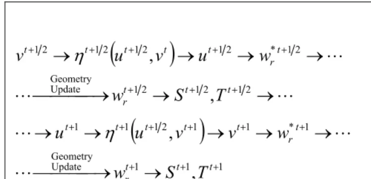
The model uses a semi-implicit ADI algorithm with two time levels per iteration. Two time schemes are currently implemented: the 4 equations S21 scheme (Abbott et al. 1973) and the 6 equations (Leendertse 1967). The time marching procedure for each discretization is depicted in figures 2-3. As usual in ADI schemes u (along x direction) is calculated implicitly in the first time level while in the second time level y becomes the implicit

direction for both elevation and velocity.

(

)

L L L ® ® ¾ ¾ ¾ ® ¾ ® ® ® + + + + + -+ + + 2 1 2 1 2 1 Update Geometry 2 1 * 1 2 1 2 1 1 2 1 , , , , t t t r t r t t t t t t T S w w u v v u u h

(

)

1 1 1 Update Geometry 1 * 2 3 2 1 2 3 1 1 , , , , + + + + + + + + + ® ¾ ¾ ¾ ® ¾ ® ® ® ® t t t r t r t t t t t t T S w w v v v u u L L L h

Figure 2. A.D.I. S21 4 equation Abbot scheme.

The free surface elevation is computed through integration of equation 1 over the water column. In each time step velocity components are used in the instant represented in figure 2. This means that in each time step one velocity component is eliminated in the free surface elevation equation, using its (discretized) evolution equation.

The Leendertse scheme is more efficient in the simulation of flows with intertidal regions because the boundary condition is calculated for both directions in each time step. The S21 scheme is more efficient in deep regions. In practice, for shallow domains, the larger time step admitted by the Leendertse scheme is almost lost due to its longer computational time.

(

)

L L L ® ® ¾ ¾ ¾ ® ¾ ® ® ® ® + + + + + + + + 2 1 2 1 2 1 Update Geometry 2 1 * 2 1 2 1 2 1 2 1 , , t t t r t r t t t t t T S w w u v u v h

(

)

1 1 1 Update Geometry 1 * 1 1 2 1 1 1 , , + + + + + + + + + ® ¾ ¾ ¾ ® ¾ ® ® ® ® ® t t t r t r t t t t t T S w w v v u u L L L h

Figure 3. A.D.I. 6 equation Leendertsee scheme. The vertical velocity component is also calculated by continuity. The integration is however performed over each cell volume. Since the grid lines are allowed to move along the vertical direction the computation of the vertical velocity field and the redefinition of the geometry are interrelated and are calculated in conjunction.

The ADI schemes produce tri-diagonal matrixes that can be efficiently solved by the Thomas algorithm. The two components of the horizontal velocity are globally centered in t+1/2 leading to a second order time accuracy.

In the finite volume method the natural choice of dependent variables are the water fluxes instead of the velocities. With this in mind the Uflux, Vflux, and Wflux will be used in the discretized form of equations 1-4, 6.

3.2 Sea level calculation

Using the finite volume approach, the discretized equations are obtained through integration on the water column of the continuity equation both in space and time. Considering a position i,j in the horizontal, the integration of equation 1 along the water column followed by integration in time from t to t+1/2 gives, with the aid of the divergence Gauss theorem:

0 2 1 2 1 = × =

_{ò ò}

ò ò

+ + t t sc t t V ijdt v ndsdt dV v ij r r r div (7)

ò

_¶ =_¶

Vij is the volume of the water column from the

surface to the bottom below position i,j, sc is the envelope surface of the water column and nr is the outward normal to sc. The surface integral computes the fluxes both in the horizontal and vertical surfaces of the envelope.

The absolute vertical velocity of the water on the free surface can be considered as the sum of the velocity of the surface and the relative velocity:

s r. Considering the water flux trough the

free surface null the vertical flux from equation 7 can be seen to represent the volume change of the water column between t and t+1/2. The discretized form of the continuity equation integrated over the water column becomes:

r r r w=w +w dt Vflux Vflux dt Uflux Uflux A dt t t k k k ij ijk t t k k k ij ijk H t ij t ij j i

ò å

ò å

+ = + + = + + ÷ ø ö ç è æ -+ ÷ ø ö ç è æ -= -2 1 _max 1 1 2 1 _max 1 1 2 1 , 1 2 h h (8)

AH = DUX ´ DVY is the projected area of the cell on the horizontal plane. The time integration is performed in conformity with the time discretization and the fluxes Uflux, Vflux are determined implicitly by the momentum equations.

3.3 Discretization of the momentum equation

The momentum equation 2 is now integrated for each cell volume i,j,k.

The time derivative term must be integrated over the control volume that is also variable in time. This can be easily done with the aid of the Leibnitz rule that, for volume integrals read:

( )

d dt f dV df dt dV f v n dS V V s S

ò

=

ò

+

ò

r r× (9)

where is the outward normal to the exterior surface S of the cell volume V and is the velocity of that surface relative to a fixed referential. The first term of equation 2 becomes:

r n _r v_s

(

)

(

)

(

)

(

) (

[

s H top s H bot

]

t ijk u t ijk u sc s V V j i j i ij ij A W U A W U t V U V U ds n v u dV u t dV t u , , 1 × × -× × - D × -× = × -+

ò

ò

r r ¶ ¶ (10)

)

where _u is the volume of the u-cell. In the last term

s represent the velocities of the top and bottom

cell faces and is determined by the vertical movement of the vertices as a function of the particular coordinate system in use. The other terms of the surface integral are not present since the cell adopted in this model do not admit horizontal movement of the lateral faces.

V W

The advective term of equation 2 is integrated with the aid of the Gauss theorem, applied to the volume in some instant of time between t and t+1:

( )

(

)

(

)

(

)

i j

(

)

ij

(

H

) (

_top H _bot ij ij Sc V ij ij ij UWA UWA Vflux U Vflux U Uflux U Uflux U dS n v u dV v u div -+ -+ + -= × = + +

ò

ò

1 1

)

r r r (11) The last term in 10 and 11 can be added producing:

(

)

[

]

[

(

)

]

(

H

) (

top H

)

bot bot H s top H s j i j i j i j i A Wr U A Wr U A W W U A W W U , , , , × × -× × = × -× -× -× (12) where Wr is the vertical velocity of the fluid measured relative to the top and bottom surfaces and

Wr´ Ah = Wflux is the water flux trough that surface. This term can be viewed as the advective fluxes entering the moving cell, the particular discretisation of this advective term depends on the scheme in use.

The other terms in equation 2 are discretized in a similar manner. The final form of the u momentum equation is:

(

)

(

)

÷÷ø ö ççè æ _{+ + + +} = × + D × -×

å

+ v difx h difx coriolx clin b x trop b x t ijk u t ijk u F F F F F flux U t V U V U . . . . 0 1 1 r (13)

Fx are the x components of the forces applied to the fluid mass due to barotropic, baroclinic, coriolis, horizontal and vertical diffusion effects.

For stability reasons the vertical transport and barotropic pressure must be implicit, all the other terms in equation 13 are calculated explicitly. Because The new level is computed before the

velocity the calculation of the barotropic term is in fact explicit in the equations without compromising stability properties.

3.4 Processes in the vertical direction

For some coordinate systems the volume Vut+1 is dependent on the hydrodynamic variables and is not known in the instant t+1 during the calculation of the horizontal velocities. For this reason the geometry changes are accounted during the computation of the vertical velocities.

The vertical velocity in each cell is calculated by continuity integrating equation 1 in the cell volume and in time as done for equation 7:

ò ò

+ + _{- =- ×} 2 1 2 1 t t sc r t ijk t ijk Vol v n ds dt Vol r r (14)

The surface integral extends to all exterior cell surfaces. The fluxes resulting from its discretization must be the same used in the momentum and elevation equations in order to ensure conservation.

The cell volume in time t+1/2 depends on the vertical coordinate in use: For sigma coordinate the volume is a function of time through _h and can be readily calculated. For isopycnic coordinate the mesh moves as a function of the density field that have not been calculated yet, finally for the lagrangean coordinate the mesh moves as a function of the vertical velocity itself and the procedure should be iterative.

In order to implement generic coordinates the vertical velocity is calculated in two steps. In the first step the value w*r is predicted assuming that the volume remains constant:

(

-

)

=-

_ò

× × × +₊ + sc h ijk ijk ij ij DVY Wr Wr v n ds DUX *t12 *t12 r r 1 (15)

The w*r value is then used, if needed, for the redefinition of the mesh geometry. The value of the vertical velocity is then corrected using the volume variation:

(

)

2 / 2 / 1 2 1 2 1 t Vol Vol ds n v Wr Wr DVY DUX t ijk t t ijk sc h ijk ijk ij ij t t D -× -= -× × D + +

ò

+ + r r (16) After evaluation of the hydrodynamic field the salinity and temperature variables are computed by integration of equation 6. In this equation the volume variation is now already known and can be used explicitly.

4 INITIAL AND BOUNDARY CONDITIONS Equations 1-4, 6 form an initial-boundary value problem requiring initial conditions in the whole domain and boundary conditions in the subsequent instants of time.

The initial conditions are of the Dirichlet type being easily implemented.

Five types of boundaries can be present in one application: free-surface, bottom, lateral closed boundary, lateral opened boundary and moving boundary.

4.1 Free surface condition

In the free-surface boundary the water flux across the surface is assumed null

0

sup =

Wflux (17)

and the wind stress is imposed n ¶ ¶ t v h W v z r _r sup = (18)

The first condition is imposed directly in the continuity equation. The wind stress is imposed explicitly in the momentum equation.

4.2 Bottom boundary condition

The conditions in the bottom boundary are similar to the free surface conditions. The water flux is also assumed null and a quadratic law is used to calculate the bottom stress:

n ¶ ¶ v h bot D h h v z C v v r r r = (19)

For stability reasons the bottom stress must be calculated implicitly in the momentum equation of the bottom cell. This is accomplished by a procedure proposed by Backhaus (1983), where the horizontal velocity of the bottom cell is used to compute vh and the stress on the top surface of the bottom cell is considered explicitly.

4.3 closed boundaries

In this boundaries the domain is limited by land. The area of that surface is much smaller than the bottom surface. Also, the horizontal resolution of this mesoscale model is larger than the characteristic dimension of the lateral boundary layer. For that

reasons a impermeable, free slip condition has been adopted in the lateral surfaces:

¶ ¶ r v n =0 (20) r r v n_{× = 0 (21)}

Using the finite volume method this is accomplished in a direct way specifying zero water fluxes and zero momentum diffusive fluxes for the cell faces in contact with land.

4.4 Lateral open boundaries

The open boundaries are introduced artificially in order to confine the computation domain to the region of interest. This procedure saves computation resources but must be used with care in order to limit the influence of the boundary condition on the domain results.

The condition to impose depends on the region where or the reason why the border has been set. In this model three types has been implemented: Imposed water flow, usually applied to rivers, Imposed free surface elevation, used in the boundaries influenced by the tide and Von Neumann boundary condition used to impose the values of salinity and temperature.

The values of S and T used in this last condition are computed as a function of the external imposed values and the interior domain values. If the flow is leaving the domain the external value is equal to the fluid property inside the domain. If the fluid, on the contrary, is entering the domain, the external value of the property is computed using a dilution length condition. In this formulation the outgoing fluid is considered to mix completely with the exterior fluid along a specified distance

If the flow is stationary this condition is equivalent to the usual restoring time condition where a restoring time after which complete mix occur is considered.

4.5 Moving boundaries

Moving boundaries are closed boundaries whose position varies with time. This type of situation arises in domains with inter-tidal zones, in this case the uncovered cells must be tracked and a condition similar to equations 20 and 21 is imposed to the surrounding covered cells. For computational reasons the condition h £ -h can not be used to decide if a cell is uncovered. Instead, a criteria based on figure 4 is used.

Figure 4. Conditions for uncovered cells

HMIN is the depth below which the cell is considered uncovered; thus conserving a thin sheet of water above the uncovered cell. The cells of position i,j are considered uncovered when at least one of the two situations is true:

and h (22) HMIN H_ij < _ij-1 <-h_ij +HMIN or and h (23) HMIN H_ij-1 < _ij <-h_ij-1 +HMIN

where H = h + h is the total depth. The second

condition of case 22 covers the cell with water when the wave propagates from the left to the right and the second condition of case 23 covers the cell when the wave propagates from the right to the left. The noise formed by the abrupt variations in velocity of the uncovered cells are controlled with a careful choice of HMIN (Leendertse 1970, Stelling 1983)

5 RESULTS

A major application of the model (MOHID3D) presented in this paper is in the Sado Estuary, Portugal. The Hydrodynamical results presented are the first phase of an environmental study, made by HIDROMOD Lda for the Setubal's Port Administration - APSS. The study's main objective is to predict the environmental effects of dredging works planned in the estuary.

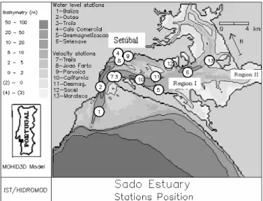
Sado Estuary, the second largest estuary in Portugal, is located some 50 Km south of Lisbon. The estuary comprises two main geographic regions as depicted in figure 5 (Rodrigues 1992):

1. The outer estuary - Region I - , with complex geometry, a surface area of about 140 km2 _{and a}

mean depth of 10 meters, and

2. The inner estuary - Region II - that comprise Alcácer's channel approximately 20 km long and about 1 meter deep.

Sado River flows into the estuary through the Alcácer channel. This river is characterized by

particularly high flow rates during very wet winters, when the discharge can reach 250 m3/s, while in dry season flow rates of 1-3 m3/s are usually recorded.

Figure 5 Sado's estuary bathymetry

5.1 Model validation

Tidal data and velocities measured in summer are available to validate the results. Because in Summer the river flow rate is small a barotropic simulation was carried out. A 120 ´ 158 points horizontal mesh with 200 meters constant horizontal step is used. Vertical discretization is based on a sigma coordinate with 6 layers.

The water level is imposed at the sea boundary using 22 harmon1ic constants from the Sesimbra tide gauge, out of the estuary (Sobral 1977). These values were obtained from 6 months data records and phases were corrected to represent correctly the values at the open boundary.

Model results are compared with field data at 6 water level stations (1 to 6 in figure 5) and 7 current meter stations (7 to 13). Each current meter station comprises a current meter located 1 meter below the surface and another one located about 3 meters above the bottom (Ribeiro & Neves 1982).

Values from July 1980 were used in the validation procedure because more data were available for that period.

In figure 6 the water level data of station 6, located in the interior of the estuary is compared with model results for the period 13 – 21 July 1980. As can be seen, the agreement is very good even for that location. Near the mouth of the estuary the agreement is even better, as should be expected.

Figure 6. Water level time series in station 6.

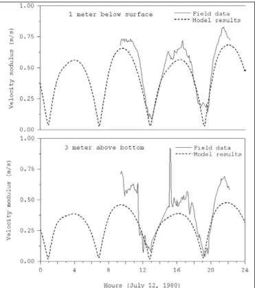
Velocity values from the model were also compared with field data. For this purpose model results were interpolated to obtain velocities at the same vertical positions as current meters.

The vertical velocity profile is of logarithmic shape for most of the tidal cycle. Tide reversion occurs earlier near the bottom putting into evidence inertial effects.

In figure 7 field data and model results are compared for station 11. Since only short period velocity records were available it was not possible to decompose the data into their constituents. Instead, the raw data were used in this comparison.

In stations located in the upper estuary where topography is more complex the agreement decreses. This fact can be explained by inaccuracies in the bathymetry, that is not measured as often as in the navigation areas.

As can be seen there is good agreement both for water slack instants and velocity values. A better agreement is obtained near the surface. This is because the bottom current meter was suspended from the boat and the measuring depth was not constant.

5.2 Qualitative verification

3D simulation of estuarine hydrodynamics opens new perspectives in the study of estuarine currents. Secondary flows in curves and slopes can be visualized, as well as the vertical structure of velocity profile and residual circulation.

The residual flow for a neap-spring half period is presented in figure 8.

Figure 7. Velocity modulus time series in station 11. Two residual circulation structures can be identified near the mouth. A clockwise eddy can be observed in the interior and a counterclockwise one on the outside. Along the main channel a strong transport towards the ocean can be identified. This pattern agrees with a physical model and field data for the region (LNEC 1989) and is a very valuable tool to explain the sediment dynamics near the estuarine mouth.

Figure 8. Residual circulation for a neap-spring cycle. As expected in a barotropic simulation, the larger vertical velocities are found in regions with strong flow curvature or with sharp topography gradients. In figure 9 a vertical cut through a region of large

bathymetry variation can be seen. The cut is located outside the estuary's mouth in a steep region adjacent to the ocean (white strip at the end of the navigation channel in the figure).

Figure 9. Vertical recirculation in a steep region. A recirculation zone behind the step can be identified in the ebb period. This recirculation must be responsible for the steepness of the slope, since during both flood and ebb in its lower part the flow tend to be slopeward.

6 FUTURE WORK

The model proved to simulate accuratly real barotropic flows. For this type of flow sigma coordinates are the most adequate since topography pays a major role.

In the next phase of this project the model will be run in baroclinic mode with different vertical discretizations and the influence of vertical discretization will be analyzed.

REFERENCES

Abbot, M. B., A. Damsgaardand & G.S Rodenhuis

1973. System 21, Jupiter, a design system for two-dimensional nearly-horizontal flows. J. Hyd. Res. 1:1-28. Adcroft, A.J., C.N. Hill & J. Marshall 1997. Representation

of Topography by Shaved Cells in a Height Coordinate Ocean Model. Mon. Weather Rev. 125:2293-2315

Backhaus, J.O. 1983. A semi-implicit scheme for the shallow water equations for application to shelf sea modelling. Continental Shelf Sea Res. 2:243-254.

Bleck, R. & D. Boudra 1986. Wind-driven spin-up in eddy-resolving ocean models formulated in isopycnic and isobaric coordinates. J. Geophys. Res. 91:7611-7621.

Bryan, K. 1969. A numerical method for the study of the circulation of the World Ocean. J. Comput. Phys. 4:347-376.

Deleersnijder, E. & E. Wolanski 1990. Du rôle de la dispersion horizontale de quantité de mouvement dans les modéles marins tridimensionnels. Proceedings of the

“Journées Numériques de Besançon - Courants Océaniques”: 39-50. Besançon: Crolet & Lesaint.

Deleersnijder, E. & J.M. Beckers 1992. On the use of the

s-coordinate system in regions of large bathymetric variations. J. Mar. Sys. 3:381-390.

Hirsch, C. 1992. Numerical computation of internal and

external flows. Numerical Methods in Engineering. Wiley

& Sons.

Leendertse, J. J. 1967. Aspects of a computational model for long water wave propagation. Rand Corporation,

Memorandum RH-5299-RR. Santa Monica.

Leendertse, J.J., 1970. A water quality simulation model for well mixed estuaries and coastal seas. Rand Corporation,

Memorandum RM-6230-RC. Santa Monica

Leendertsee, J.J. & S.K. Liu 1978. A three-dimensional turbulent energy model for non-homogeneous estuaries and coastal sea systems. In J.C.J. Nihoul (ed.),

Hydrodynamics of Estuaries and Fjords: 387-405.

Amsterdam: Elsevier.

LNEC 1989. Estudo da barra do Sado – Projecto do

Modelo Físico. Laboratório Nacional de Engenharia

Civil. Lisboa

Oberhuber, J.M. 1993. Simulation of the Atlantic circulation with a coupled Sea Ice – Mixed Layer – isopycnal General Circulation Model. Part I: Model description. J.

Phys. Oceanogr. 23(5):830-845.

Phillips, N.A. 1957. A coordinate system having some special advantages for numerical forecasting. J. Meteorol. 14:184-185.

Ribeiro, M.C. & R.J.J Neves 1982. Caracterização

hidrográfica do estuário do Sado. Departamento de

Engenharia Mecânica, IST. Lisboa.

Rodrigues, A.M.J. 1992. Environmental status of a multiple

use estuary, through the analysis of benthic communities: the Sado estuary, Portugal. PhD. Thesis. University of

Stirling.

Santos, A. 1985. Modelo hidrodinâmico tridimensional de

circulação oceânica e estuarina. PhD. Thesis. IST.UTL.

Lisboa.

Sobral, J.T. 1977. Estuário do Sado - Observação de

correntes de marés. Instituto Hidrográfico. Lisboa.

Stelling, G.S. 1983. On the construction of computational

methods for shallow water flow problems. Ph.D. Thesis,

Technische Hogeschool to Delft.

Versteeg, H. & W. Malalasekera 1995. An introduction to

computational fluid dynamics, the finite volume method.

New York: Longman Scientific & Technical.

Vinokur, M. 1989. An analysis of finite-difference and finite-volume formulations of conservation laws. J.