www.the-cryosphere.net/4/1/2010/
© Author(s) 2010. This work is distributed under the Creative Commons Attribution 3.0 License.
The Cryosphere
Interaction between ice sheet dynamics and subglacial lake
circulation: a coupled modelling approach
M. Thoma1,2, K. Grosfeld2, C. Mayer1, and F. Pattyn3
1Bavarian Academy and Sciences, Commission for Glaciology, Alfons-Goppel-Str. 11, 80539 Munich, Germany 2Alfred Wegener Institute for Polar and Marine Research, Bussestrasse 24, 27570 Bremerhaven, Germany
3Laboratoire de Glaciologie, D´epartement des Sciences de la Terre et de l’Environnement (DSTE), Universit´e Libre de
Bruxelles (ULB), CP 160/03, Avenue F.D. Roosevelt, 1050 Bruxelles, Belgium
Received: 15 September 2009 – Published in The Cryosphere Discuss.: 29 September 2009 Revised: 15 December 2009 – Accepted: 15 December 2009 – Published: 8 January 2010
Abstract.Subglacial lakes in Antarctica influence to a large
extent the flow of the ice sheet. In this study we use an ide-alised lake geometry to study this impact. We employ a) an improved three-dimensional full-Stokes ice flow model with a nonlinear rheology, b) a three-dimensional fluid dynamics model with eddy diffusion to simulate the basal mass bal-ance at the lake-ice interface, and c) a newly developed cou-pler to exchange boundary conditions between the two in-dividual models. Different boundary conditions are applied over grounded ice and floating ice. This results in signif-icantly increased temperatures within the ice on top of the lake, compared to ice at the same depth outside the lake area. Basal melting of the ice sheet increases this lateral tempera-ture gradient. Upstream the ice flow converges towards the lake and accelerates by about 10% whenever basal melting at the ice-lake boundary is present. Above and downstream of the lake, where the ice flow diverges, a velocity decrease of about 10% is simulated.
1 Introduction
During the last decades our knowledge on subglacial lake systems has greatly increased. Since the discovery of the largest subglacial lake, Lake Vostok (Oswald and Robin, 1973; Robin et al., 1977), more than 270 other lakes have been identified so far (Siegert et al., 2005; Carter et al., 2007; Bell, 2008; Smith et al., 2009). Plenty of efforts have been undertaken to reveal partial secrets subglacial lakes may hold, mostly referring to Lake Vostok. For instance the spec-ulation that extremophiles in subglacial lakes may be en-countered (e.g., Duxbury et al., 2001; Siegert et al., 2003) has
Correspondence to:M. Thoma ([email protected])
been nurtured by microorganisms discovered in ice core sam-ples (Karl et al., 1999; Lavire et al., 2006). These samsam-ples originate from the at least 200 m thick accreted ice, drilled at the Russian research station Vostok (Jouzel et al., 1999). Discussions about the origin and history of the lake (Duxbury et al., 2001; Siegert, 2004; Pattyn, 2004; Siegert, 2005) are still ongoing. It is still unknown whether Subglacial Lake Vostok existed prior to the Antarctic glaciation and if it could have survived glaciation, or whether it formed subglacially after the onset of glaciation. The impact of subglacial lakes on the flow of the overlying ice sheet has been analysed (Kwok et al., 2000; Tikku et al., 2004, e.g.,) and modelled (Mayer and Siegert, 2000; Pattyn, 2003; Pattyn et al., 2004; Pattyn, 2008), but self-consistent numerical models, which include the modelling of the basal mass balance, are lacking at present. Several numerical estimates and models (West and Carmack, 2000; Williams, 2001; Walsh, 2002; Mayer et al., 2003; Thoma et al., 2007, 2008b; Filina et al., 2008) as well as laboratory analogues (Wells and Wettlaufer, 2008) of water flow within the lake have been carried out, permit-ting insights into the water circulation, energy budget and basal processes at the lake-ice interface. Finally, observa-tions (Bell et al., 2002; Tikku et al., 2004) and numerical modelling (Thoma et al., 2008a) of accreted ice at the lake-ice interface gave insights about its thickness and distribution over subglacial lakes.
However, current knowledge about the interaction be-tween subglacial lakes and the overlying ice sheet is lack-ing. The most important parameter exchanged between ice and water is heat. The exchange of latent heat associated with melting and freezing dominates heat conduction, but the latter process has also be accounted for in subglacial lake modelling (Thoma et al., 2008b). Melting and freezing is closely related to the ice draft which varies spatially over subglacial lakes (Siegert et al., 2000; Studinger et al., 2004; Tikku et al., 2005; Thoma et al., 2007, 2008a, 2009a). The ice draft, and hence the water circulation within the lake, is maintained by the ice flow across lakes. Without this flow, lake surfaces would even out (Lewis and Perkin, 1986). On the other hand, a spatially varying melting/freezing pattern will have an impact on the overlying ice sheet as well. In or-der to get an insight in the complex interaction processes be-tween the Antarctic ice sheet and subglacial lakes, this study for the first time couples a numerical ice-flow and a lake-flow model with a simple asynchronous time-stepping scheme to overcome the problem of different adjustment time scales.
We describe the applied ice-flow model RIMBAYand lake-flow model ROMBAXin the first two Sections, respectively. Each section starts with a general description of the partic-ular model, describes the applied boundary conditions, and the results of the uncoupled model runs. The newly devel-oped RIMBAY–ROMBAX–coupler RIROCOis introduced in Sect. 4, where we also discuss the impact of a coupled ice-lake system on the ice flow and ice-lake geometry.
2 Ice model RIMBAY
2.1 General description
The ice sheet model RIMBAY (Revised Ice sheet Model Based on frAnk pattYn) is based on the work of Pattyn (2003), Pattyn et al. (2004) and Pattyn (2008). Within this thermomechanically coupled, three-dimensional, full-Stokes ice model, a subglacial lake is represented numerically by a vanishing bottom-friction coefficient ofβ2=0, while high friction in grounded areas is represented by a large coeffi-cient; in this study we useβ2=106. The choice of the latter parameter has no influence on the model results as long as it is much larger than zero.
The constitutive equation, governing the creep of poly-crystalline ice and relating the deviatoric stressesτ to the strain ratesε˙, is given by Glen’s flow law: ε˙=Aτn (e.g., Pattyn, 2003), with a temperature dependent rate factorA=
A(T ). Here we apply the so-called Hooke’s rate factor
(Hooke, 1981). Experimental values of the exponent n in Glen’s flow law vary from 1.5 to 4.2 with a mean of about 3 (Weertman, 1973; Paterson, 1994); ice models traditionally assumen=3. However, a simplified viscous rheology with
n=1 stabilises and accelerates the convergence behaviour
of the implemented numerical solvers. Therefore, previous subglacial lake simulations within ice models were limited to viscous rheologies (Pattyn, 2008).
2.2 Model setup and boundary conditions
The model domain used in this study is a slightly enlarged version of the one presented in Pattyn (2003): It consists of a rectangular 168 100 km2large domain with a model resolu-tion of 5 km (resoluresolu-tions of 2.5 km and 10 km are also used for comparison) and 41 terrain-following vertical layers. The surface of the initially 4000 m thick ice sheet has an initial slope of 2% (similar to Lake Vostok, Tikku et al., 2004) from left (upstream) to right (downstream). An idealized circu-lar lake with a radius of about 48 km and an area of about 7200 km2 is located in the center of the domain, where a 1000 m deep cavity modulates the otherwise smoothly sloped bedrock (similar to Pattyn, 2008). The lake’s maximum wa-ter depth of about 600 m, resulting in a volume of about 1840 km3(the lake’s geometry is also indicated in Figs. 3, 4). We apply a constant surface temperature of−50◦C at the ice’s surface, a typical value for central Antarctica (Comiso, 2000). The bottom layer boundary temperature depends on the basal condition: above bedrock a Neumann boundary condition is applied, based on a geothermal heat flux of 54 mW/m2 (a value suggested for the Lake Vostok region by Maule et al., 2005). Assuming isostasy above the sub-glacial lake, the bottom layer temperature is at the pressure-depended freezing point. This temperature, prescribing a Dirichlet boundary condition, depends on the local ice sheet thickness (Tb= −H×8.7×10⁻⁴◦C/m ,e.g., Paterson, 1994). Accumulation and basal melting/freezing are ignored during the initial experiments in this Sect., where no coupling is ap-plied. In the subsequent coupling-experiments, basal melting and freezing at the lake’s interface, as modelled by the lake flow model, is accounted for (Sect. 4).
The lateral boundary conditions are periodic, hence values of ice thicknesses, velocities, and stresses are copied from the upstream (left) side to the downstream (right) side of the model domain and vice versa. The same applies to the lateral borders along the flow. The initial integration starts from an isothermal state. The basal melt rate is set to zero over bedrock as well as over the lake.
2.3 Model improvements
Compared to Pattyn (2008) we improved the model RIMBAY
0.0 0.2 0.4 0.6 0.8 1.0
Scaled friction coefficient
β
2
0 50 100 150 200 250 300 350 400
X−distance (km)
(3/2) Smoothed β2
(1/0) Smoothed β2
(0/0) Unsmoothed β2
a)
Weight factor
400
0.0 0.2 0.4 0.6 0.8
Weight factor
−5 −4 −3 −2 −1 0 1 2 3 4 5
Node distance
b)
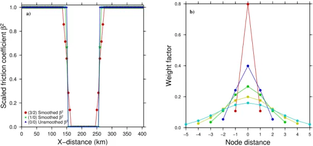
Fig. 1. (a)Friction coefficientβ2(scaled to the maximum of 106) along the central x-axis for an unsmoothed and two test-smoothed cases.
The smoothing coefficient (x/y) represents the number of nodes smoothed outside and inside of the lake’s border, respectively. (b)Weight
factors for a Gaussian-type filter with different width from one (red) to five (cyan) depending on the distance to the central node located at zero.
0 50
100 150
200 250
300 350
400
Y (km)
0 50 100 150
200 250 300
350 400
X (km)
Smooth β2:
Gaussian filter:(0/0)0
a)
0 50
100 150
200 250
300 350
400
Y (km)
0 50 100 150
200 250 300
350 400
X (km)
Smooth β2:
Gaussian filter:(1/0)2
b)
0 50
100 150
200 250
300 350
400
Y (km)
0 50 100 150
200 250 300
350 400
X (km)
Smooth β2:
Gaussian filter:(3/2)5
c)
0 2 4 6 8 10
105β
19 20 21 22 23 24
log(η)
Fig. 2. Logarithm of viscosityηof the surface layer and bedrock-friction parameter β2for an idealized model. (a)Noβ2-smoothing
or Gaussian filtering. (b)Slightβ2-smoothing (1/0) and Gaussian filtering with a filter width of two. (c)Strongβ2-smoothing (3/2) and
Gaussian filtering with a filter width of five. Note that the Figs. represent the initial conditions for a FS-model with the applied filter and
β2-smoothing.
coefficient of(1/0)is suited to decrease the integration time significantly and stabilises the numerical results. In this no-tation, (1) indicates one lubricated node on the bedrock side of the boundary and (0) indicates no stiffed (debris) node on the lake side. If the number of lubricated nodes is reduced to zero, the model’s integration time increases without a sig-nificant impact on the velocity field. If the number of stiffed nodes over the lake is increased, lower velocities over the lake are achieved. However, for higher model resolutions than used in this study, higherβ-values should be considered to make the transition more realistic.
(a) (b)
0 100 200 300 400
y (km)
0 100 200 300 400
x (km) −80
−80
−20 −20
1.2m/a
0 300 600
Lake Depth (m)
0 100 200 300 400
y (km)
0 100 200 300 400
x (km) −80
−80
−20 −20
1.2m/a
0 300 600
Lake Depth (m)
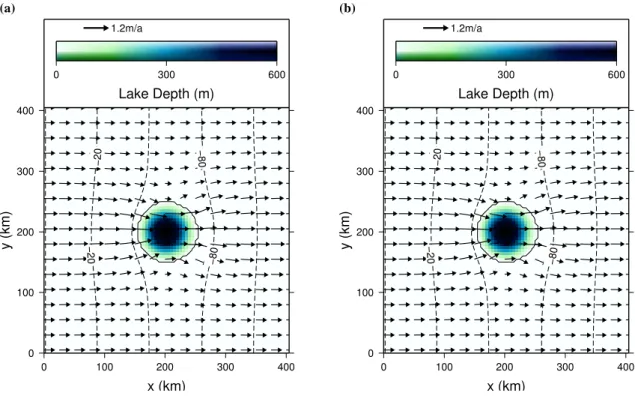
Fig. 3.Results for a full-Stokes ice dynamic model with a horizontal resolution of 5 km. (a)Lake depth (color), ice sheet surface elevation
(dashed contours), and ice-flow velocity (black arrows).(b)Vertically averaged horizontal velocity of the standard full-Stokes experiment.
2.4 Results
The standard experiment is a thermomechanically coupled full-Stokes (FS) model with a horizontal resolution of 5 km. A quasi-steady state is reached after 300 000 years. Figure 3a shows the lake’s position and depth in the center of the model domain. The frictionless boundary condition over the lake results in an increased velocity, not only above the lake, but also in it’s vicinity (Fig. 3b). From mass conservation it fol-lows, that the (vertically averaged) horizontal velocity con-verges towards the lake from upstream and dicon-verges down-stream. The flattened ice sheet surface over the lake is a con-sequence of the isostatic adjustment. This effect is also visi-ble in the geometry of the profiles in Fig. 4 and in particular in Fig. 5. The inclined lake-ice interface is maintained by the constant ice flow over the lake and hence, independent of a possible basal mass exchange.
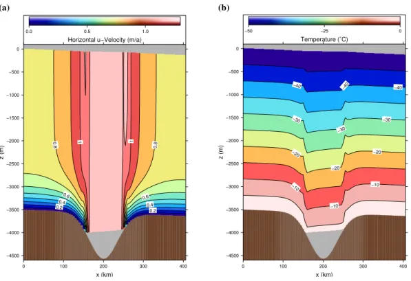
Figure 3b shows the vertically averaged horizontal veloc-ity and Fig. 4a a vertical cross section of the velocveloc-ity along the flow at the lake’s center aty=200 km. Over the lake, the ice sheet behaves like an ice shelf, featuring a verti-cally constant velocity. Towards the lake, the surface veloc-ity increases by more than 70% from about 0.7 m/a to about 1.2 m/a. The largest velocity gradients occur in the vicinity of the grounding line (Figs. 3b, 4a, 5). Convergence of ice towards the lake results in an accelerated ice flow which un-dulates at the lake’s edges because of significant changes in
the ice thickness and ice sheet surface gradients (yellow and red line in Fig. 5, respectively). The surface velocity (green line in Fig. 5) accelerates towards the lake until the ice sheet surface flattens. The velocity increase in deeper layers close to the bedrock (blue line in Fig. 5) is suspended just before the frictionless lake interface is reached, because of a strong increase of the ice thickness filling the trough. The maximum velocity is reached across the lake (Figs. 3b, 4a, 5), where the basal friction is zero. The vertical temperature profile (Fig. 4b) is nearly linear, as accumulation and basal melting are neglected. Geothermal heat flux is not sufficient to melt the bottom of the grounded ice, but over the lake the freezing point is maintained by the boundary condition. This results in submerging isotherms. At the downstream grounding line a slight overshoot of the upwelling isotherm is observed.
2.5 Robustness of the results
(a) (b)
0.2
0.2
0.4
0.4
0.6
0.6 0.8
0.8
1
1
0.0 0.5 1.0
Horizontal u−Velocity (m/a)
−4500 −4000 −3500 −3000 −2500 −2000 −1500 −1000 −500 0
z (m)
0 100 200 300 400
x (km)
−40
−40 −40
−30
−30
−30
−20
−20
−20
−10
−10
−10
−50 −25 0
Temperature (˚C)
−4500 −4000 −3500 −3000 −2500 −2000 −1500 −1000 −500 0
z (m)
0 100 200 300 400
x (km)
Fig. 4.Results for a full-Stokes ice dynamic model with a horizontal resolution of 5 km. (a)Lake depth (color), ice sheet surface elevation
(dashed contours), and ice-flow velocity (black arrows).(b)Horizontal downstream velocity (in x-direction).(c)Temperature profile.
0.0 0.5 1.0
0 50 100 150 200 250 300 350 400
x (km)
Ice Sheet Surface Ice Thickness Bedrock Friction 0.0
0.5 1.0
Surface Velocity Bedrock Velocity
Fig. 5.Cross sections alongy=200 km across the lake’s center. Shown are the normalized variables bedrock friction, ice sheet surface, and ice thickness (lower panal) as well as the corresponding velocities at the surface and close to the bedrock (upper panal).
velocity maximum at the grounding line (Fig. 5) cannot be resolved with the 10 km resolution. The finer 2.5 km model resolution needs a much longer integration time, without pro-ducing significant differences in the results compared to the intermediate 5 km grid resolution.
(a) (b)
25
25
26
26
27 27
0 40 80
20 25 30 35
Heat Cond.
mW/m2
N
−1
−0.6
−0.2 0.2
0.6 1
0 40 80
−1 0 1
Stream Function
mSv
N
(c) (d)
−1.2 −0.9
−0.9
−0.6 −0.6
−0.6 −0.3
−0.3
−1 0 1
Meridional Overturning
mSv −60
60
60
120 120
180 180
240
−300 0 300
Zonal Overturning
µSv
−12
−10
−8
−6
−4
0 40 80
−12 0 12
Basal Mass Balance
mm/a
N
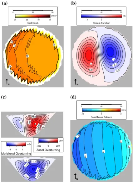
Fig. 6. (a)Heat conduction into the ice (QIce).(b)Vertically integrated mass transport stream function, positive values indicate a clockwise
circulation, negative values an anticlockwise circulation.(c)Zonal (from west to east) and meridional (from south to north) overturning.
(d)Basal mass balance.
geometry as well as the parametrization are kept identical. Our experiments indicate a moderate impact on the ice flow: calculated velocities across the subglacial lake are about 5% lower compared to the full-Stokes model. In the vicinity of the lake, the impact of the full-Stokes terms decreased, but is still enhanced along the flowlines. Although the FS-model implements more mathematics in the numercial code it con-verges faster than the higher order model, hence all further studies are performed with the full-Stokes model.
3 Lake flow model ROMBAX
3.1 General description
8 M. Thoma et al.: Coupled ice- and lake-flow
R
O
M
B
A
X
R
I
R
O
C
O
R
IM
B
A
Y
Initial Ice thickness Bedrock height Lake Geometry
RIMBAY
Restart Ice geometry Ice temperature Ice flow
Output/Input Ice thickness Water column thickness Temperature gradient
Initial
Geothermal heat ROMBAX
Out-/Input Freezing rate Melting rate
Restart Water temperature
RIMBAY
(restart)
extrap. melt/freeze
rates
ROMBAX
(restart) extrap.
tracer Output/Input Ice thickness Water column thickness Temperature gradient
Fig. 7.Couple scheme schematics. The upper part represents the ice-flow model RIMBAY, the lower part the lake-flow model ROMBAX. In
the middle the parameters exchanged by the coupler RIROCOare shown. The gray lines in the left part of the Fig. represent the initial start-up
sequence (the two initial model runs), dashed loops indicate cycles (successive model runs) that may repeat an apriori unspecified number of times. Two additional yellow ovals indicate the individual model needs regarding successive restarts/coupling: The ice flow calculated by RIMBAYmay result in new lake nodes. For these nodes the basal mass balance is calculated by averaging adjacent nodes. For ROMBAX a modified geometry desires the extrapolation of temperatures (and other tracers) from a previous model run to skip the time-consuming spin-up process.
3.2 Model setup and boundary conditions
The bedrock topography and the ice draft, needed for the lake-flow model ROMBAX, is obtained from the output (Sect. 2.4) of the ice-flow model RIMBAY (see Sect. 4 for further details). The horizontal resolution (0.025◦×0.0125◦, about 0.7×1.4 km), the number of vertical layers (16), as well as the horizontal and vertical eddy diffusivities (5 m2/s and 0.025 cm2/s, respectively) are adopted from a model of subglacial Lake Concordia (Thoma et al., 2009a). In a model domain of about 170×88×16 grid cells the circula-tion within the lake as well as the melting and freezing rates at the lake-ice interface are calculated. At the bottom of the lake a geothermal heat flux of 54 mW/m2, consistent with the ice-flow model’s boundary condition, is applied. Pre-vious subglacial lake simulations of Lake Vostok (Thoma et al., 2007, 2008a; Filina et al., 2008), Lake Concordia (Thoma et al., 2009a), or Lake Ellsworth (Woodward et al., 2009) used a prescribed average heat conduction into the ice (QIce=dT /dz×2.1 W/(K m)), based on borehole
tempera-ture measurements and thickness temperatempera-ture-gradient esti-mates. The availability of the results of the thermomechani-cal ice-sheet model RIMBAYpermits a spatially varyingQIce
(Fig. 6a). Across the lake’s center, a general draft-following
gradient from about 27 mW/m2 on the upstream side of ice flow to about 24 mW/m2on the downstream side results from the modelled temperature distribution in the ice (Fig. 4b) and is used as input for the lake-flow model.
3.3 Results
4 Coupling
4.1 General description
The bedrock topography and the ice draft, necessary to set up the geometry for the lake-flow model ROMBAX (Sect. 3.2), was obtained from the modelled output geometry of the ice-flow model RIMBAY (Sect. 2.4). In addition, the thermo-dynamic boundary condition of the heat conduction into the ice was calculated from the temperature gradient at the ice sheet’s bottom. The left part of Fig. 7 (gray lines) shows schematically the performed operations. A coordinate con-version is necessary as RIMBAY uses Cartesian coordinates while ROMBAXis based on spherical coordinates.
The modelled melting and freezing rates (Fig. 6d) are considered to replace the previously zero-constrained lower boundary condition in the ice-flow model RIMBAY (indi-cated by the central triangle within the yellow area in Fig. 7). Again a coordinate transformation is necessary. To speed up the integration time, ice geometry, ice flow, and ice temper-ature from the initial model run are reused (indicated by the black-lined triangle within the blue area within Fig. 7). An additional process has to be considered since the lake’s area may change during an ice-model run. As the basal mass bal-ance (melting/freezing) depends on the former lake-model results and cannot be calculated during a specific model run, extrapolation of neighbouring values may be necessary (indi-cated by the embedded yellow oval in the blue area of Fig. 7). In each coupling cycle, successive initialisations of the lake-flow model ROMBAX are performed with the slightly changed ice draft and water column thickness (indicated by the right triangle in the yellow area of Fig. 7), as well as the temperature field of the previous model-run (indicated by the central triangle in the orange area of Fig. 7). Because the lake flow model does not permit dynamically changing geometry, temperatures of emerging nodes have to be extrapolated from neighbouring nodes (indicated by the embedded yellow oval in the orange area of Fig. 7). It is not necessary to reuse (and possibly extrapolate) the water circulation, as this value is based on the tracer (density) distribution and converges quickly.
The coupling mechanism, including initial starts of the individual models, parameter exchanges, coordinate trans-formations, and restart-initialisations are embedded into and controlled by the RIMBAY–ROMBAX–Coupler RIROCO.
In Sect. 2.4 and Sect. 3.3 the results of the initial runs of the individual models have been described. So far the only parameter exchange beween both models was the uni-lateral initilisation of the lake flow model ROMBAXwith the modelled geometry and temperature gradient of the ice flow model RIMBAY(indicated by the gray lines in Fig. 7). The real coupling procedure starts, when the results of ROMBAX
are reinserted into RIMBAY(indicated by the black lines in Fig. 7).
4.2 Results
From ROMBAXthe basal mass balance at the ice sheet-lake interface is considered for subsequent initialisations of RIM
-BAY. Melting dominates freezing (which is negligible) and hence the ice sheet is loosing mass. Note that the molten ice does not affect the lake’s volume, neither in the ice-sheet model nor in the lake-flow model, as this is constant per defi-nition. This mass imbalance can be interpreted as a virtual constant water flow out of the lake without any feedback to the ice sheet. The coupler RIROCOapplies restarts from previous model runs. Consequently the models reach their new quasi-steady state after a significant shorter integration time. Ice sheet volume in the model domain is decreasing by about 600 km3per 100 000 years, equivalent to about 3.5 m
thickness. Ice draft reduction in the lake-flow model within 100 000 years is shown in Fig. 8a. Most ice is lost in the cen-ter of the lake (up to 8 m), and the area of maximum mass loss is slightly shifted to the upstream side of the lake. Con-sequently, the water column thickness increases where most ice is molten and decreases where less ice is molten (Fig. 8b). However, the ice-thickness reduction and slope adjustment is too small to change the surface pressure on the lake water, and hence the water flow, significantly. Just a few iteration cycles are needed to bring this coupled lake-water system into a quasi-steady state.
(a)
(b)
−7
−3
0 40 80
−10 −5 0
Ice Thickness
m
N
−2.8 −1.2
−1.2
0.2
1
0 40 80
−4 −2 0 2
Water Column
m
N
(c)
(d)
−0.3
−0.3
−0.3
−0.3
0 40 80
−1.0 −0.5 0.0 0.5 1.0
Basal Mass Balance
mm/a
N
25 25
26 26
27 27
28
28
29
29
30
30
31
31
32
32
33 33 33
33
0 40 80
20 25 30 35
Heat Cond.
mW/m2
N
Fig. 8.Impact of melting after 100 000 years on(a)the ice draft,(b)the water column thickness, and(c)the basal mass balance. Shown is
the geometry difference between the lake-flow model restart and the initial geometry.(d)Indicates the heat conduction into the ice (QIce).
5 Summary
Observations from space show that large subglacial lakes have a significant impact on the shape and dynamics of the Antarctic Ice Sheet as they flatten the ice sheets surface (Siegert et al., 2000; Kwok et al., 2000; Leonard et al., 2004; Tikku et al., 2004; Siegert, 2005). These regions depict a change in surface slope due to the isostatic adjustment of the ice sheet. This, combined with the lacking bottom friction, results in an observable redirection of ice flow. In this study, we apply a newly coupled ice sheet-lake flow model on an idealized ice sheet-lake configuration to investigate the feed-backs between the individual systems. The full-Stokes ice sheet model (Pattyn, 2008) is improved to handle a more re-alistic non-linear rheology. The lake-flow model is based on
a three dimensional fluid dynamics model with eddy diffu-sivity and simulates the lake flow as well as the mass bal-ance at the lake-ice interface. This model, previously only applied to lake-exclusive studies with a prescribed ice thick-ness and bedrock, now receives its geometry directly from the ice flow model. In addition, heat flux from the lake into the ice sheet is an exchange parameter. Besides other exter-nal forcing fields, the ice-flow model receives the basal mass balance at the interface from the dynamic lake-flow model.
In order to stabilise the ice-flow model numerically with a nonlinear rheology, a slight Gaussian filtering of the ice viscosity is necessary.
(a) (b)
−0.05
−0.05
−0.05
−0.01
−0.01
−0.01
−0.01
−0.01
−0.01
−0.10 −0.05 0.00 0.05 0.10 Horizontal u−Velocity (m/a)
−4500 −4000 −3500 −3000 −2500 −2000 −1500 −1000 −500 0
z (m)
0 100 200 300 400
x (km)
−1.1
−1.1
−1.1
−1.1
−1.1 −1.1 −0.22
−0.22
−0.22
−0.22
−0.22
−0.22
−0.22
−0.22
−0.22
−0.22
−0.22
−0.22
−2 −1 0 1 2
Temperature (˚C)
−4500 −4000 −3500 −3000 −2500 −2000 −1500 −1000 −500 0
z (m)
0 100 200 300 400
x (km)
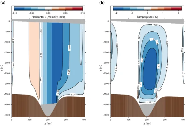
Fig. 9.Differences between coupled-model result and initial model (Fig. 4) for(a)horizontal downstream velocity and(b)temperature.
of the deceleration when the flow reaches the bedrock again. Melting at the lake-ice interface increases the ice flow accel-eration upstream and decreases the ice flow on top of the lake as well as downstream, because of the reduced surface slope. This impacts on the velocity can be traced about 75 km up-and downstream of the lake in this specific setting, which corresponds to about 20 times the ice sheet thickness. The temperature at the ice sheet bottom on top of the lake is at the pressure melting point, and hence warmer than the bedrock-based ice in the vicinity. According to our simulation, melt-ing at the lake-ice interface reduces the temperature on top of the lake. Advection transports the relatively colder ice down-stream, and hence the temperature dependent rheology will have impacts on the ice flow beyond the lake.
Our idealised configuration of an ice-lake system indicates an important impact of the interaction between both systems on the ice sheet’s dynamics. Next applications of this new coupled model will focus on realistic configurations, such as Lake Vostok and its glacial drainage system. In order to in-vestigate the flow dynamical impact which can be compared with observations.
Acknowledgements. This work was funded by the DFG through
grant MA3347/2-1. The authors wish to thank Saito Fuyuki,
Povl Christoffersen, and an anonymous reviewer for helpful comments as well as Andrea Bleyer for proof reading.
Edited by: I. M. Howat
References
Bell, R. E.: The role of subglacial water in ice-sheet mass balance, Nat. Geosci., 1, 297–304, doi:10.1038/ngeo186, 2008.
Bell, R. E., Studinger, M., Tikku, A. A., Clarke, G. K. C., Gutner, M. M., and Meertens, C.: Origin and fate of Lake Vostok water frozen to the base of the East Antarctic ice sheet, Nature, 416, 307–310, 2002.
Carter, S. P., Blankenship, D. D., Peters, M. E., Young, D. A., Holt, J. W., and Morse, D. L.: Radar-based subglacial lake classification in Antarctica, Geochem. Geophys. Geosyst., 8, doi:10.1029/2006GC001408, 2007.
Comiso, J. C.: Variability and trends in Antarctic surface tempera-tures from in situ and satellite infrared measurements, J. Climate, 13, 1674–1696, 2000.
Duxbury, N. S., Zotikov, I. A., Nealson, K. H., Romanovsky, V. E., and Carsey, F. D.: A numerical model for an alternative origin of Lake Vostok and its exobiological implications for Mars, J. Geophys. Res., 106, 1453–1462, 2001.
Filina, I. Y., Blankenship, D. D., Thoma, M., Lukin, V. V., Masolov, V. N., and Sen, M. K.: New 3D bathymetry and sediment distri-bution in Lake Vostok: Implication for pre-glacial origin and nu-merical modeling of the internal processes within the lake, Earth Pla. Sci. Let., 276, 106–114, doi:10.1016/j.epsl.2008.09.012, 2008.
Fricker, H. A., Scambos, T., Bindschadler, R., and Padman, L.: An active subglacial water system in west Antarctica mapped from space, Science, 315, 1544–1548, doi:10.1126/science.1136897, 2007.
R., and Jezek, K.: Evidence for subglacial water transport in the West Antarctic Ice Sheet through three-dimensional satellite radar interferometry, Geophys. Res. Lett., 32, 3, doi:10.1029/2004GL021387, 2005.
Griffies, S. M.: Fundamentals of ocean climate models, Princeton University Press, Princeton, 2004.
Grosfeld, K., Gerdes, R., and Determann, J.: Thermohaline circu-lation and interaction beneath ice shelf cavities and the adjacent open ocean, J. Geophys. Res., 102, 15595–15610, 1997. Holland, M. D. and Jenkins, A.: Modeling Thermodynamic
Ice-Ocean Interaction at the Base of an Ice Shelf, J. Phys. Ice-Oceanogr., 29, 1787–1800, 1999.
Hooke, R. L.: Flow law for polycrystalline ice in glaciers: Com-parison of theoretical predictions, laboratory data, and field mea-surements, Rev. Geophys. Space Phys., 19, 664–672, 1981. Inman, M.: Antarctic drilling: The plan to unlock Lake Vostok,
Sci-ence, 310, 611–612, doi:10.1126/science.310.5748.611, 2005. Jouzel, J., Petit, J. R., Souchez, R., Barkov, N. I., Lipenkov,
V. Y., Raynaud, D., Stievenard, M., Vassiliev, N. I., Verbeke, V., and Vimeux, F.: More than 200 meters of lake ice above subglacial Lake Vostok, Antarctica, Science, 286, 2138–2141, doi:10.1126/science.286.5447.2138, 1999.
Karl, D. M., Bird, D. F., Bjrkman, K., Houlihan, T., Shack-elford, R., and Tupas, L.: Microorganisms in the accreted ice of Lake Vostok, Antarctica, Science, 286, 5447, 2144–2147, doi:10.1126/science.286.5447.2144, 1999.
Kwok, R., Siegert, M. J., and Carsey, F. D.: Ice motion over Lake Vostok, Antarctica: constraints on inferences regarding the ac-creted ice, J. Glaciol., 46, 689–694, 2000.
Lavire, C., Normand, P., Alekhina, I., Bulat, S., Prieur, D., Bir-rien, J., Fournier, P., Hnni, C., and Petit, J.: Presence of Hy-drogenophilus thermoluteolus DNA in accretion ice in the sub-glacial Lake Vostok, Antarctica, assessed using rrs, cbb and hox., Environ. Microbiol., 8, 2106–2114, doi:10.1111/j.1462-2920.2006.01087.x, 2006.
Leonard, K., Bell, R. E., Studinger, M., and Tremblay, B.: Anomalous accumulation rates in the Vostok ice-core resulting from ice flow over Lake Vostok, Geophys. Res. Lett., 31, 24, doi:10.1029/2004GL021102, 2004.
Lewis, E. L. and Perkin, R. G.: Ice pumps and their rates, J. Geo-phys. Res., 91, 11756–11762, 1986.
Marshall, S. J.: Recent advances in understanding ice sheet dynam-ics, Earth Pla. Sci. Let., 240, 191–204, 2005.
Maule, C. F., Purucker, M. E., Olsen, N., and Mosegaard, K.: Heat Flux Anomalies in Antarctica Revealed by Satellite Magnetic Data, Science, 309, 464–467, doi:10.1126/science.1106888, 2005.
Mayer, C. and Siegert, M. J.: Numerical modelling of ice-sheet dy-namics across the Vostok subglacial lake, central East Antarctica, J. Glaciol., 46, 197–205, doi:10.3189/172756500781832981, 2000.
Mayer, C., Grosfeld, K., and Siegert, M.: Salinity impact on wa-ter flow and lake ice in Lake Vostok, Antarctica, Geophys. Res. Lett., 30, 1767, doi:10.1029/2003GL017380, 2003.
Oswald, G. K. A. and Robin, G. d. Q.: Lakes Beneath the Antarctic Ice Sheet, Nature, 245, 251–254, doi:10.1038/245251a0, 1973. Paterson, W. S. B.: The Physics of Glaciers, Butterworth
Heine-mann, Oxford, 3 Edn., 1994.
Pattyn, F.: A new three-dimensional higher-order
thermomechan-ical ice sheet model: Basic sensitivity, ice stream development, and ice flow across subglacial lakes, J. Geophys. Res., 108, 1–15, doi:10.1029/2002JB002329, 2003.
Pattyn, F.: Comment on the comment by M. J. Siegert on “A nu-merical model for an alternative origin of Lake Vostok and its exobiological implications for Mars” by N. S. Duxbury et al., J. Geophys. Res., 109, E11004, doi:10.1029/2004JE002329, 2004. Pattyn, F.: Investigating the stability of subglacial lakes with a full Stokes ice-sheet model, J. Glaciol., 54, 353–361, doi:10.3189/002214308784886171, 2008.
Pattyn, F., de Smedt, B., and Souchez, R.: Influence of subglacial Vostok lake on the regional ice dynamics of the Antarctic ice sheet: a model study, J. Glaciol., 50, 583–589, 2004.
Robin, G. D. Q., Drewry, D. J., and Meldrum, D. T.: International Studies of Ice Sheet and Bedrock, Philos. Tr. R. Soc., 279, 185– 196, 1977.
Saito, F., Abe-Ouchi, A., and Blatter, H.: Effects of first-order stress gradients in an ice sheet evaluated by a three-dimensional thermomechanical coupled model, Ann. Glaciol., 37, 166–172, doi:10.3189/172756403781815645, 2003.
Schiermeier, Q.: Russia delays Lake Vostok drill, Antarctica’s hid-den water will keep its secrets for another year, Nature, 454, 258– 259, doi:10.1038/454258a, 2008.
Siegert, M. J.: Comment on “A numerical model for an alterna-tive origin of Lake Vostok and its exobiological implications for Mars” edited by: Duxbury, N. S., Zotikov, I. A., Nealson, K. H., Romanovsky, V. E., and Carsey, F. D., J. Geophys. Res., 109, 1–3, doi:10.1029/2003JE002176, 2004.
Siegert, M. J.: Reviewing the origin of subglacial Lake Vostok and its sensitivity to ice sheet changes, Prog. Phys. Geog., 29, 156– 170, doi:10.1191/0309133305pp441ra, 2005.
Siegert, M. J., Kwok, R., Mayer, C., and Hubbard, B.: Water ex-change between the subglacial Lake Vostok and the overlying ice sheet, Nature, 403, 643–646, doi:10.1038/35001049, 2000. Siegert, M. J., Tranter, M., Ellis-Evans, J. C., Priscu, J. C., and
Lyons, W. B.: The hydrochemistry of Lake Vostok and the po-tential for life in Antarctic subglacial lakes, Hydr. Proc., 17, 795– 814, 2003.
Siegert, M. J., Hindmarsh, R., Corr, H., Smith, A., Woodward, J., King, E. C., Payne, A. J., and Joughin, I.: Subglacial Lake Ellsworth: A candidate for in situ exploration in West Antarc-tica, Geophys. Res. Lett., 31, 1–4, doi:10.1029/2004GL021477, 2004.
Siegert, M. J., Carter, S., Tabacco, I. E., Popov, S., and Blanken-ship, D. D.: A revised inventory of Antarctic subglacial lakes, Anatarct. Sci., 17, 453–460, doi:10.1017/S0954102005002889, 2005.
Smith, B. E., Fricher, H. A., Joughin, I. R., and Tulaczyk, S.: An in-ventory of active subglacial lakes in Antarctica detected by ICE-Sat (2003–2008), J. Glaciol., 55, 573–595, 2009.
Studinger, M., Bell, R. E., and Tikku, A. A.:
Estimat-ing the depth and shape of subglacial Lake Vostok’s water cavity from aerogravity data, Geophys. Res. Lett., 31, 12, doi:10.1029/2004GL019801, 2004.
Thoma, M., Grosfeld, K., and Lange, M. A.: Impact of the Eastern Weddell Ice Shelves on water masses in the eastern Weddell Sea, J. Geophys. Res., 111, doi:10.1029/2005JC003212, 2006. Thoma, M., Grosfeld, K., and Mayer, C.: Modelling mixing and
cir-culation in subglacial Lake Vostok, Antarctica, Ocean Dynamics, 57, 531–540, doi:10.1007/s10236-007-0110-9, 2007.
Thoma, M., Grosfeld, K., and Mayer, C.: Modelling accreted ice in subglacial Lake Vostok, Antarctica, Geophys. Res. Lett., 35, 1–6, doi:10.1029/2008GL033607, 2008a.
Thoma, M., Mayer, C., and Grosfeld, K.: Sensitivity of Lake Vos-tok’s flow regime on environmental parameters, Earth Pla. Sci. Let., 269, 242–247, doi:10.1016/j.epsl.2008.02.023, 2008b. Thoma, M., Filina, I., Grosfeld, K., and Mayer, C.: Modelling flow
and accreted ice in subglacial Lake Concordia, Antarctica, Earth Pla. Sci. Let., 286, 278–284, doi:10.1016/j.epsl.2009.06.037, 2009a.
Thoma, M., Grosfeld, K., and Lange, M. A.: Modelling the im-pact of ocean warming on Eastern Weddell Ice Shelf melting and water masses in their vicinity, Ocean Dynamics, re-submitted, 2009b.
Thoma, M., Grosfeld, K., Smith, A. M., and Mayer, C.: A com-ment on the equation of state and the freezing point equation with respect to subglacial lake modelling, Earth Pla. Sci. Let., submitted, 2009c.
Tikku, A. A., Bell, R. E., Studinger, M., and Clarke, G. K. C.: Ice flow field over Lake Vostok, East Antarctica in-ferred by structure tracking, Earth Pla. Sci. Let., 227, 249–261, doi:10.1016/j.epsl.2004.09.021, 2004.
Tikku, A. A., Bell, R. E., Studinger, M., Clarke, G. K. C., Tabacco, I., and Ferraccioli, F.: Influx of meltwater to subglacial Lake Concordia, east Antarctica, J. Glaciol., 51, 96–104, 2005. Walsh, D.: A note on eastern-boundary intensification of flow in
Lake Vostok, Ocean Modelling, 4, 207–218, 2002.
Weertman, J.: Creep of ice, in: Physics and Chemistry of Ice, edited by Whalley, E., Jones, S. J., and Gold, L. W., pp. 320–337, Royal Society of Canada, Ottawa, 1973.
Wells, M. G. and Wettlaufer, J. S.: Circulation in Lake Vostok: A laboratory analogue study, Geophys. Res. Lett., 35, 1–5, doi:10.1029/2007GL032162, 2008.
Williams, M. J. M.: Application of a three-dimensional numerical model to Lake Vostok: An Antarctic subglacial lake, Geophys. Res. Lett., 28, 531–534, 2001.
Williams, M. J. M., Grosfeld, K., Warner, R. C., Gerdes, R., and Determann, J.: Ocean circulation and ice-ocean interaction be-neath the Amery Ice Shelf, Antarctica, J. Geophys. Res., 106, 22383–22400, 2001.
Wingham, D. J., Siegert, M. J., Shepherd, A., and Muir, A. S.: Rapid discharge connects Antarctic subglacial lakes, Nature, 440, 1033–1036, doi:10.1038/nature04660, 2006.
Woodward, J., Smith, A. M., Ross, N., Thoma, M., Siegert, M. J., King, M. A., Corr, H. F. J., King, E. C., and Grosfeld, K.: Bathymetry of Subglacial Lake Ellsworth, West Antarctica and implications for lake access, Geophys. Res. Lett., in preparation, 2009.