Collective coordinate analysis for double sine-Gordon model
Samira Nazifkar∗ and Kurosh Javidan† Department of physics, Ferdowsi university of Mashhad
91775-1436 Mashhad Iran
(Received on 6 December, 2009)
Collective coordinate analysis for adding a space dependent potential to the double sine-Gordon model is presented. Interaction of solitons with a delta function potential barrier and also delta function potential well is investigated. Most of the features of interaction are derived analytically. We will find that the behaviour of a solitonic solution is like a point particle which moves under the influence of a complicated effective potential. The effective potential is a function of the field initial conditions and also parameters of added external potential.
Keywords: Topological solitons; Double sine-Gordon; Collective coordinate
1. INTRODUCTION
Topological solitons are important objects in various areas of physics and mathematics. Solitons widely appear in non-linear classical field theories as stable, particle-like objects, with finite mass and smooth structures. They are localized in space as the energy density of these objects is nonzero only in a finite region; i.e. it is significantly nonzero in a small region and goes to zero, exponentially or as an inverse power, as one moves away from this region. They are stable due to nontrivial topological properties of the vacuum mani-fold. These coherent nonperturbative excitations are distinct from the perturbative excitation objects which correspond to localized small field oscillations around the vacuum [1, 2]. Solitonic picture of baryons in high energy physics and also Skyrme solitons in nuclear physics are examples of particle-like bahaviour of topological solitons [3, 4] Finding suitable methods for the point representation of soliton solutions of the hierarchies of non-linear evolution equations is an inter-esting subject in nonlinear field theory (for example see [5]). In this paper we will deal with on of these models.
The sine-Gordon model is probably the most studied inte-grable model. This model describes a large variety of physical systems ranging from the Josephson effects, particle physics, information transport in microtubules [6], nonlinear optics [7], crystal dislocations [8], and ferromagnets [9]. Double sine-Gordon (DSG) model arises as a sine-Gordon type field theory bearing solitonic solutions with important applications and also attractive mathematical properties. DSG model has been used in describing a multibaryon system. So their solu-tions appear in the multiflaver spectrum and some resonances inQCD2[10]. There is a very near Relation between DSG model and deformed quantum AshkinTeller model which de-scribes quantum Ising spin chain system [11]. Interacting pair of resistively shunted Josephson junctions and fluxon dynam-ics in long Josephson junctions are modeled using a DSG for-mulation [12–14]. Quantum noise of ferromagneticπ-Bloch Domain Walls also describes using a model with DSG theory [15].
In the inhomogeneous version of the sine-Gordon model, the coefficient in front of the potential becomes a function of space. Recently, there has been an increasing interest in
∗Electronic address:[email protected]
†Electronic address:[email protected]
the scattering of solitons from defects or impurities, which generally come from medium properties. It is very interesting to examine the methods of adding the potential to the model on the DSG as a non-integrable model.
Interaction of solitons with defects mainly investigates us-ing numerical analysis and numerical simulations. Some an-alytical models have been presented which are constructed with using suitable collective coordinate variables. Collec-tive coordinate analysis for point representation of solitons of single sine-Gordon model has been studied before [16, 17]. In this paper collective coordinate system for DSG model is presented for the first time. The results are more interesting than the single sine-Gordon model, because of very attrac-tive shape of the field potential of DSG model. This system is constructed base on the method of adding the defects by mak-ing some parameters of the equation of motion to be function of space.
2. SOLITONS OF DOUBLE SINE-GORDON EQUATION
Lagrangian of the double sine-Gordon model in (1+1) di-mensions is defined by
L
=12∂µφ∂
µφ
−λ(2−cosφ−cos 2φ) (1)
where µ=0,1. The field equation of motion from the La-grangian (1) is:
∂µ∂µφ+λ(sinφ+2 sin 2φ) =0 (2)
One soliton solution for the DSG equation can be written as [18, 19].
φ(x,X(t)) =kπ−2tan−1
1
√
5sinh
√
5
√
λ(x−X(t))
1−X˙2
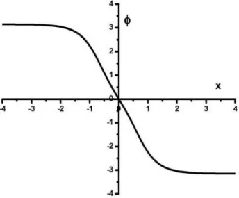
(3) whereX(t) =x0−Xt˙ .x0and ˙Xare soliton initial position and its velocity respectively. It is a kink-like solution as figure 1 shows.
FIG. 1: Kink-like solution of DSG equation (2) as a function of position
found by subtracting usual value ofλ=1 fromλ(x). Param-eterλ(x)has been used in [2] as follows
λ(x) =
1+λ0 |x| ≤p 1 |x|>p
(4)
This means that potential V(x) is a rectangular function with the width of ’p’ and the heightλ0. Solution (3) withλ=1 can be used as initial condition for solving (2) when the potential V(x) is small.
By inserting the solution (3) (withλ=1) in the Lagrangian (1), using adiabatic approximation [22] we have
L
=X˙2−1−λ(x)50 cosh2√5(x−X(t))
5+sinh2√5(x−X(t)) 2 (5)
3. COLLECTIVE COORDINATE VARIABLE
The center of a soliton can be considered as a particle, if we look at this variable as a collective coordinate. The col-lective coordinate could be related to the potential by using the Lagrangian (5). This model is able to give us an analytic solution for most of the features of the soliton-potential sys-tem. X(t) remains as a collective coordinate if we integrate Lagrangian (5) over the variable x. If we take the potential V(x) =εδ(x)(λ(x) =1+εδx) then (5) becomes
L=
L
dx=M02
˙
X2−2−
50εcosh2√5X
5+sinh2√5X 2
(6)
where
M0 = ∞
−∞
100 cosh2√5(x−X(t))
5+sinh2√5(x−X(t)) 2 dx
= ln
5+2√5 5−2√5
+4√5 (7)
The equation of motion for the variable X(t) is derived from (6) as
M0X¨−100ε√5
× ⎛
⎜ ⎝
cosh
√
5X sinh
√
5X
3−sinh2
√
5X
5+sinh2√5X 3
⎞
⎟ ⎠=0
(8) The above equation shows that the peak of the soliton moves under the influence of a complicated force which is a function of external potentialV(x)and soliton position. Ifε>0 we have a barrier andε<0 creates a potential well. Figure 2 shows effective force as a function of position forε=0.1. Fortunately equation (8) has an exact solution as follows
FIG. 2: Effective force acted on the collective particle as a function of position withε=0.1.
1 2M0
˙
X2−X˙02+50ε
× ⎛
⎜ ⎝
cosh2√5X
5+sinh2√5X 2
− cosh
2√ 5X0
5+sinh2√5X0 2
⎞
⎟ ⎠=0
(6) as follows
E=1 2M0X˙
2+M0+50ε cosh 2√5X
5+sinh2√5X 2
(10)
It is the energy of a particle with the mass ofM0and velocity ˙
X which is moved under the influence of external effective potential. ThereforeM0is indeed the rest mass of one soliton solution (3) of DSG. Figure 3 presents effective potential en-ergy density of a static soliton as a function of its position un-der the influence of the potentialV(x) =εδ(x)withε=0.1. Thus the effective force is a conservative force and can be described using the effective potential. Equation (10) shows that the effective potential isEP=50ε
cosh2(√5X)
(5+sinh2(√5X))2 . From
the marginal behaviour of hyperbolic functions at infinity, one can show that the potential decays to zero exponentially when X goes to infinity. Potential energy has two absolute maxima and one local minimum which can be found by finding the ze-ros of the effective force. As figure 2 presents, effective force become zero at the origin (center of the external potential) which is the local minimum of the potential.Potential energy reaches its maximum values atXmax=±cosh
−1(2)
√
(5) . Maximum energy of the soliton isEmax=12M0X˙2+M0+5016ε. Because
of the extended nature of the soliton, the effective potential is not an exact delta function. By substituting ˙X from (9) into
FIG. 3: Collective energy density as a function of position for a static soliton in a delta-like external potential withε=0.1.
(10) one can show that the energy is a function of soliton ini-tial conditionsX0and ˙X0only. Therefore the energy of the system is conserved.
Topological charge is [23]
Q= 1 2π
−∞
+∞
∂φ
∂XdX (11)
where ∂∂φX is topological charge density. For the solution (3)
we have
∂φ ∂X =
10 cosh√5X 5+sinh2√5X
(12)
Collective topological charge Q can be calculated by Integrat-ing (12) over the variable X. A simple calculation shows that topological charge of one soliton solution isQ=1 which is constant and independent of X.
Some features of soliton-potential dynamics can be inves-tigated using equations (9) and (10) analytically which are discussed in the next sections.
4. POTENTIAL BARRIER
Suppose that a delta-like potential barrier with the height εis located at the origin. There are two different kinds of behaviour for the soliton, during the interaction with the ef-fective potential barrier. It depends on its initial location and its initial velocity. If the soliton is far away from the potential (|X0|>Xmax) the soliton reflects back or passes over the
bar-rier depends on its initial velocity. Also there is an interesting situation which has not been observed before. If soliton initial position is near to the center of the potential (say|X0|<Xmax)
the soliton is trapped by the barrier and oscillate around the center of the potential, if it has low initial velocity. These situations have been explained in detail in the following.
When the soliton is far from the center of the potential (X→∞) (10) reduces toE=1
2M0X˙02+M0, where ˙X0 is its initial velocity at infinity. It is the energy of a particle with the rest massM0and the velocity of ˙X0. A soliton with a low velocity reflects back from the barrier and a high energy soli-ton climbs over the barrier and passes through it. So we have a critical value for the velocity of the soliton which separates these two situations. The energy of a soliton at theXmax is E(X =Xmax) =12M0X˙2+M0+5016ε. The minimum energy for a soliton in this position isE=M0+5016ε. On the other hand, a soliton which comes from infinity with initial veloc-ityvc has the energy of E(X=∞) = 21M0v2c+M0. There-fore the minimum velocity for the soliton to pass the barrier isvc= 52
ε
M0. The same result is derived by substituting
˙
X=0, ˙X0=vc,X0=∞andX=0 in (10).
If the soliton is located at some position likeX0(which is not necessary infinity) the critical velocity will not be52Mε
0.
Soliton passes over the barrier if the soliton energy is greater than the energy of a static soliton at Xmax. So a soliton at
the initial positionX0with initial velocity ˙X0has the critical initial velocity if its velocity becomes zero atX=Xmax.
Con-sider a soliton with initial conditions ofX0and ˙X0. If we set X=Xmaxand ˙X=0 in equation (9) thenvc=X0˙ . Therefore
we have
vc=
100ε M0
⎛
⎜ ⎝
1 16−
cosh2√5X0
5+sinh2√5X0 2
⎞
⎟
⎠ (13)
po-sition far away from the external potential has critical velocity of 52Mε
0.
FIG. 4: Critical velocity as a function of initial positionX0 with ε=0.1M0.
If soliton at infinity has initial velocity less than thevcthen
there exists a return point in which the velocity of the soliton is zero. For this situation we have
cosh2√5Xstop
5+sinh2√5Xstop 2=
M0 100εX˙
2
0 (14)
Therefore this model predicts linear relation between poten-tial strengthεand ˙X02. Equation (14) shows that complicated term cosh
2(√5X
stop)
(5+sinh2(√5Xstop))2
has linear relation with ˙X02and also 1
ε.
A soliton with initial conditionsX0and ˙X0 will go to in-finity after the interaction with a potential barrier. The final velocity of the soliton at infinity after the interaction is
˙ X= ˙ X2 0+ 100ε M0
cosh2√5X0
5+sinh2√5X0
2 (15)
which is greater than the initial velocity ˙X0.
Equations (9) and (10) show that the soliton finds its initial velocity after the interaction when it reaches its initial posi-tion. This means that the interaction is completely elastic.
5. SOLITON-WELL SYSTEM
The soliton-well system is very interesting problem. Sup-pose a particle moves toward a frictionless potential well. It
falls in the well with an increasing velocity and reaches the bottom of the well with its maximum speed. After that, it will climb the well with decreasing velocity and finally pass through the well. Its final velocity after the interaction is equal to its initial speed. But there are some differences be-tween point particle and a soliton in a potential well. Our an-alytic model explains several features of soliton-well system correctly.
Changingεto−εin (6) changes potential barrier to poten-tial well. The solution for the system is
1 2M0
˙
X2−X˙02−50ε
× ⎛
⎜ ⎝
cosh2√5X
5+sinh2√5X 2
− cosh
2√5X 0
5+sinh2√5X0 2
⎞
⎟ ⎠=0
(16) There is not a critical velocity for a soliton-well system, but we can define an escape velocity. A soliton with initial po-sitionX0reaches the infinity with a zero final velocity if its initial velocity is
˙ Xescape=
100ε M0
cosh2√5X0
5+sinh2√5X0
2 (17)
In other words, a soliton which is located at the initial position X0can escape to infinity if its initial velocity ˙X0is greater than the escape velocity ˙Xescape.
The X(t), trajectory of a soliton during the interaction with the potential well follows from (16) as
t= X(t)
X(t=0)
⎛ ⎜ ⎜ ⎝ ˙
X02+100ε M0
cosh2√5X0
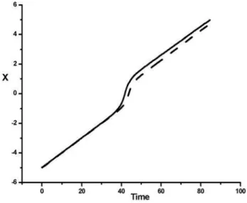
5+sinh2√5X0 2 ⎞ ⎟ ⎟ ⎠ −1 dx (18) The above integral has been evaluated numerically by us-ing Rumberg’s method and X(t) was plotted versus t. This result was compared with direct simulation using equation (2). Figure 4 shows the result for a system withX0=−5,
˙
X0=−0.1 andε=−0.2. There is a little difference between
the predicted final velocities from different models after the interaction. The difference is reduced when the height of the potential(ε) reduces. The difference is due to the approxima-tion which is used for deriving (5) from (1).
Consider a potential well with the depth ofεand a soliton at the initial positionX0which moves toward the well with initial velocity ˙X0smaller than the ˙Xescape. The soliton
inter-acts with the potential and reaches a maximum distanceXmax
from the center of the potential with a zero velocity and then come back toward the well. The soliton oscillates around the well with the amplitudeXmax. The required initial velocity to
FIG. 5: Soliton trajectory during the interaction with potential well. Potential depthε=−0.2 has been chosen for direct simulation using (2) (solid line) and(ε=−0.134)using analytic model (dash line). Initial conditions areX0=−5 and ˙X0=0.1
˙ X0=
100ε M0
⎛
⎜ ⎝
cosh2√5X0
5+sinh2√5X0 2−
cosh2√5Xmax
5+sinh2√5X
max 2
⎞
⎟
⎠ (19)
If the initial velocity is lower than the escape velocity the soliton oscillates around the well. The period of oscillation can be calculated numerically using equation (16).
6. CONCLUSION AND REMARKS
An analytical model for the scattering of double sine-Gordon solitons from delta function potential barriers and also potential wells has been presented. Several features of soliton-potential characters were calculated using this model. A critical velocity for the soliton during the interaction with a potential barrier as a function of its initial conditions and the potential characters has been found. The model predicts specific relations between some functions of initial conditions and other functions of final state of the soliton after the
inter-action . An escape velocity has been derived for the soliton-well system. Oscillation period of a soliton in a potential soliton-well also has been discussed using this model.
Presented collective coordinate method is able to explain most of the features of double sin-Gordon soliton system dur-ing the interaction with an external potential. But this model (like analytical model for single sine-Gordon model in Ref. [16] or presented analytical model forφ4in Ref.[21]) is not able to explain fine structure of the islands of trapping in soliton-well system. This phenomenon is a very interesting features of soliton-potential systems. It is expected to find an acceptable explanation for this behaviour using a better model with suitable collective coordinate method. On the other hand using this method for investigation of other nonlinear models in potentials is an interesting subject.
[1] Manton N. and Sutcliffe P. ’Topological Solitons’ Cambridge university press UK. 2004
[2] Al-Alawi Jassem H. , Zakrzewski W.J. (2007) J. Phys. A40, 11319
[3] Christova C.V.,Blotza A.,Kim H.C.,Pobylitsaa P.,Watabea T.,Meissnerd Th.,Ruiz Arriolae E. and Goeke K. 1996 Prog.Part.Nucl.Phys. 37
[4] Panico G.,Wulzer A. 2009 Nuclear Physics A82591114
[5] Biaszak M. 1987 J. Phys. A: Math. Gen.20L1253-L1255 [6] Abdalla E.,Maroufia B.,Melgara B. C. and Sedrab M. B. 2001
Physica A301, 169
[7] McCall S. and Hahn E. L. 1969 Phys. Rev.183, 457 [8] Frenkel J. and Kontorova T., 1939 J. Phys. [Moscow]1137 [9] Wysin G., Bishop A. R. and Kumar P.,1984 J. Phys. C17, 5975 [10] Harold B., 2007 J. High Energy Phys. JHEP03,055
Physics B580[FS], 647687
[12] Werner P, Refael G and Troyer M 2005 J. Stat. Mech. P12003 [13] Hatakenaka N.,Takayanagi H., Kasai Y. and Tanda S. 2000
Physica B284-288563-564
[14] Giuliano1 D. and Sodano P., 2009 arXiv: 0908.0913 [15] Crompton P.R., 2008 arXiv:0810.2087
[16] Javidan K. 2008 PHYS. REV. E78, 046607 [17] Ghahraman A., Javidan K. 2008 Arxiv:0809.0210 [18] Wazwaz A. 2006 Phys. Lett. A350367370
[19] Mussardo G., Riva V., Sotkovc G., 2004 Nuclear Physics B687
[FS] (2004) 189219
[20] Piette B., Zakrzewski W.J. 2007 J. Phys. A: Math. Theor.40No 2, 329-346
[21] Hakimi E. and Javidan K., 2009 PHYS. REV. E80, 016606 [22] Kivshar Y. S. , Fei Z. and Vasquez L. 1991 Phys. Rev. Lett67
1177