Abstract—This paper coordinates pricing and inventory replenishment decisions in a multi-level supply chain composed of multiple suppliers, one manufacturer and multiple retailers. We model this problem as a three-level nested Nash game where all the suppliers formulate the bottom-level Nash game, the whole supplier sector play the middle-level Nash game with the manufacturer, and both sectors as a group player formulate the top-level Nash game with the retailers. Analytical method and solution algorithm are developed to determine the equilibrium of the game. A numerical study is conducted to understand the influence of different parameters on the decisions and profits of the supply chain and its constituent members. Several interesting research findings have been obtained.
Index Terms—pricing, replenishment, multi-level supply chain, Nash game.
I. INTRODUCTION
In the decentralized supply chain, inconsistence and incoordination existed between local objectives and the total system objectives make the supply chain lose its competitiveness increasingly ([10]). Many researchers have recommended organizational coordination for managing supply chain efficiently ([1, 3, 5, 12]). Integrating pricing with inventory decisions is an important aspect to manufacturing and retail industries.
Coordinating pricing and inventory decisions of supply chain (CPISC) has been studied by researchers at about fifty years ago. Weng and Wong [15] and Weng [14] propose a model of supplier-retailer relationship and confirm that coordinated decisions on pricing and inventory benefit both the individual chain members and the entire system. Reference [2] analyzes the problem of coordinating pricing and inventory replenishment policies in a supply chain consisting of a wholesaler, one or more geographically dispersed retailers. They show that optimally coordinated policy could be implemented cooperatively by an inventory-consignment agreement. Prafulla et al. [11] present a set of models of coordination for pricing and order quantity decisions in a one manufacturer and one retailer supply chain. They also discuss the advantages and disadvantages of various coordination possibilities. The research we have discussed above, mainly focus on coordination of individual entities or two-stage channels. In reality, a supply chain usually consists of multiple firms (suppliers, manufacturers, retailers, etc). Jabber and Goyal [6] consider coordination of order quantity in a multiple suppliers, a single vendor and
Manuscript received September 6, 2010.
Yun Huang is with the Department of Industrial and Manufacturing Systems Engineering, University or Hong Kong, Hong Kong (phone: (00852) 64851458; e-mail: [email protected]).
George Q. Huang is with the Department of Industrial and Manufacturing Systems Engineering, University or Hong Kong, Hong Kong (e-mail: [email protected])
multiple buyers supply chain. Their study focuses on coordination of inventory policies in three-level supply chains with multiple firms at each stage.
Recently, Game Theory has been used as an alternative to analyze the marketing and inventory policies in supply chain wide. Weng [13] study a supply chain with one manufacturer and multiple identical retailers. He shows that the Stackelberg game guaranteed perfect coordination considering quantity discounts and franchise fees. Yu et al. [17] simultaneously consider pricing and order intervals as decisions variable using Stackelberg game in a supply chain with one manufacturer and multiple retailers. Esmaeili et al. [4] propose several game models of seller-buyer relationship to optimize pricing and lot sizing decisions. Game-theoretic approaches are employed to coordinate pricing and inventory policies in the above research, but the authors still focus on the two-stage supply chain.
In this paper, we investigate the CPISC problem in a multi-level supply chain consisting of multiple suppliers, a single manufacturer and multiple retailers. The manufacturer purchases different types of raw materials from his suppliers. Single sourcing strategy is adopted between the manufacturer and the suppliers. Then the manufacturer uses the raw materials to produce different products for different independent retailers with limited production capacity. In this supply chain, all the chain members are rational and determine their pricing and replenishment decisions to maximize their own profits non-cooperatively.
We describe the CPISC problem as a three-level nested Nash game with respect to the overall supply chain. The suppliers formulate the bottom-level Nash game and as a whole play the middle-level Nash game with the manufacturer. Last, the suppliers and the manufacturer being a group formulate the top-level Nash game with the retailers. The three-level nested Nash game settles an equilibrium solution such that any chain member cannot improve his profits by acting unilaterally without degrading the performance of other players. We propose both analytical and computational methods to solve this nested Nash game.
This paper is organized as follows. The next section gives the CPISC problem description and notations to be used. Section 3 develops the three-level nested Nash game model for the CPISC problem. Section 4 proposes the analytical and computational methods used to solve the CPISC problem in Section 3. In section 5, a numerical study and corresponding sensitivity analysis for some selected parameters have been presented. Finally, this paper concludes in Section 6 with some suggestions for further work.
Joint Pricing and Inventory Replenishment
Decisions in a Multi-level Supply Chain
II. PROBLEM STATEMENT AND NOTATIONS A. Problem description and assumptions
In the three-level supply chain, we consider the retailers facing the customer demands of different products, which can be produced by the manufacturer with different raw materials purchased from the suppliers. These non-cooperative suppliers reach an equilibrium and as a whole negotiate with the manufacturer on their pricing and inventory decisions to maximize their own profits. After the suppliers and the manufacturer reach an agreement, the manufacturer will purchase these raw materials to produce different products for the retailers. Negotiation will also be conducted between the manufacturer and the retailers on their pricing and inventory decisions. When an agreement is achieved between them, the retailers will purchase these products and then distribute to their customers. We then give the following assumptions of this paper:
(1) Each retailer only sells one type of product. The retailers’ markets are assumed to be independent of each other. The annual demand function for each retailer is the decreasing and convex function with respect to his own retail price.
(2) Solo sourcing strategy is adopted between supplies and manufacturer. That is to say, each supplier provides one type of raw materials to the manufacturer and the manufacturer purchases one type of raw material from only one supplier.
(3) The integer multipliers mechanism [9] for replenishment is adopted. That is, each supplier’s cycle time is an integer multiplier of the cycle time of the manufacturer and the manufacturer’s replenishment time is the integer multipliers of all the retailers.
(4) The inventory of the raw materials for the manufacturer only occurs when production is set up.
(5) Shortage are not permitted, hence the annual production capacity is greater than or equal to the total annual market demand ([4]).
B. Notations
All the input parameters and variables used in our models will be stated as follow. Assume the following relevant parameters for the retailer:
L: Total number of retailers
l
r
: Index of retailer l lr
A
: A constant in the demand function of retailer l, which represents his market scalel
r
e
: Coefficient of the product’s demand elasticity for retailer ll
r
p
: Retail price charged to the customer by retailer ll
r
D
: Retailer l’s annual demandl
r
R
: Retailer l’s annual fixed costs for the facilities and organization to carry this productl
r
X
: Decision vectors set of retailer l.l l
r r
x
X
is his decision vector.l
r
Z
: Objective (payoff) function of retailer lThe retailer’s decision variables are:
l
r
G
: Retailer l’s profit marginl
r
k
: The integer divisor used to determine the replenishment cycle of retailer lThe manufacturer’s relevant parameters are:
m: Index of manufacturer
l
mp
h
: Holding costs per unit of product l inventorysv
mr
h
: Holding costs per unit of raw material purchased from supplier vm
S
: Setup cost per productionm
O
: Ordering processing cost per order of raw materialsl
P
: Annual production capacity product l, which is a known constantm
R
: Manufacturer’s annual fixed costs for the facilities and organization for the production of this productl
m
p
: Wholesale price charged by the manufacturer to the retailer ll
m
c
: Production cost per unit product l for the manufacturerm
X
: Decision vectors set of the manufacturer.m m
x
X
is his decision vector.m
Z
: Objective (payoff) function of the manufacturer The manufacturer’s decision variables are:l
m
G
: Manufacturer’s profit margin for product lT
: Manufacturer’s setup time interval The relevant parameters for the supplier are:V: Total number of suppliers
v
s
: Index of supplier v, v=1,2,…,V vs
h
: Holding costs per unit of raw material inventory for supplier vv
s
c
: Raw material cost paid by supplier v vs
R
: Supplier v’s annual fixed costs for the facilities and organization to carry the raw materialv
s
O
: Order processing cost for supplier v per orderv
s
: Usage of supplier v’s raw material to produce a unit product lv
s
p
: Raw material price charged by supplier v to the manufacturerv
s
X
: Decision vectors set of supplier v.v v
s s
x
X
is his decision vector.v
s
Z
: Objective (payoff) function of supplier vThe supplier’s decision variables are:
v
s
G
: Supplier v’s profit marginv
s
III. MODEL FORMULATION A. The three-level nest Nash game scheme
We model the CPISC problem as a three-level nested Nash game with V+ L+1 players, i.e., V suppliers, one manufacturer and L retailers. Each supplier controls decision vectors set
v
s
X
(v=1,2,…,V) to maximize his payoff functionv
s
Z
. A decision vectorv v
s s
x
X
includes profit marginv
s
G
and replenishment decisionsv
s
K
. Themanufacturer controls the decision vectors set
X
m to maximize his payoff functionZ
m . His decision vectorm m
x
X
consists of profit marginl
m
G
for different product l (l=1,2,…L) and setup time interval T. Each retailer controls the decision vectors setl
r
X
, whose decision vectorl l
r r
x
X
is composed of profit marginl
r
G
and replenishment decisionsl
r
k
, to maximize his payoff functionl
r
Z
.In our game framework, firstly, the V suppliers formulate the bottom-level Nash game. Given the manufacturer’s and the retailers’ decision vectors, each supplier’s decision vector
v v s s
x X varies with the change of the other suppliers’ decision vectors to maximize his payoff function
v
s
Z
. When none of them would like to alter their decisions, the bottom-level Nash equilibrium is obtained. Secondly, the suppliers in equilibrium being a player formulate the middle-level Nash game with the manufacturer. In this game, given the retailers’ decision vectors, the suppliers adjust theirdecision vectors
1,..., V
s s s
x x x with the change of the manufacturer’s decisions, while the manufacturer varies his decision vector xmXm as the suppliers’ decisions changing until none of them could improve his payoff function by unilaterally altering his decisions. Thus, the middle-level Nash equilibrium achieves. Lastly, the top-level Nash game is played between the suppliers and the manufacturer in equilibrium and all the retailers. Each retailer’s decision vector
l l
r r
x
X
varies with the change of the suppliers’ and the manufacturer’s decisions and the other retailers’ decisions. The suppliers and the manufacturer also adjust their equilibrium decision vectors
x x
s,
m
with the change of the retailers’ decisions. The process continues until the suppliers, the manufacturer and the retailers cannot increase their payoffs by changing their decisions. That is the top-level Nash equilibrium reaches.B. The retailers’ model
We first consider the objective (payoff) function
l
r
Z
for the retailers. The retailer’s objective is to maximize his net profit by optimizing his profit marginl
r
G
and replenishment decisionl
r
k
.As indicated in the fourth point of the assumption in section 2.1, the integer multipliers mechanism is employed
between the manufacturer and the retailers. Since the setup time interval for the manufacturer is assumed to be T, the replenishment cycle for retailer l is
/
l
r
T k
.l
r
k
should be a positive integer. Thus, the annual holding cost is/ 2
l l l
r r r
h TD
k
(see Fig. 1(a)) and the ordering process cost is/
l lr r
O k
T
.lv l sTDr
lu l
sTDr
l
l r
r
TD k
v lv l s s r
l
KT
DThe retailer l faces the holding cost, the ordering cost and an annual fixed cost. Therefore, the retailer l’s objective function is given by the following equation:
, 2
max l l l
l l l l l
l
rl rl
r r r
r r r r r
r
k G
TD O k
Z G D h R
k T
, (1) Subject to
{1, 2, 3,...}
l
r
k , (2)
l l l
r r m
G p p , (3)
l l l l r r r r
D A e p , (4)
Grl0, (5)
0 l r l
D P
. (6) Constraint (2) shows the demand function. Constraint (3) gives the value of the divisor used to determine the retailer l’s replenishment cycle time. Constraint (4) indicates the relationship between the prices (the retail price and the wholesale price) and retailer l’s profit margin. Constraint (5) ensures that the value of
l
r
C. The manufacturer’s model
The manufacturer’s objective is to determine his decision vector
x
m, composed of the profit margins for all the productsl
m
G and the setup time interval for production T, to
maximize his net profit.
The manufacturer faces annual holding costs, setup and ordering costs, and an annual fixed cost. The annual holding cost for the manufacturer is composed of two parts: the cost of holding raw materials used to convert to products, the cost of holding products. During the production portion, the average inventory of raw material v used for product l is
/ 2
lv ls
TD
r
. The production time in a year is/
lr l
D
P
.During the non-production portion of the cycle, the raw materials inventory drops to zero and the holding cost is zero according to our assumption. Hence, the annual holding cost for raw material v is
2
/ 2
sv lv l
mr s r l
h
T D
P
. The annualinventory for product l’s is given by 1 1 2
l l
l r r
r l
D T
D
k P
(as suggested by [8]). The behavior of the inventory level for the manufacturer is illustrated as Fig. 1(b). The setup cost
m
S
and ordering costO
moccur at the beginning of each production. Thus, we can easily derive the manufacturer’s objective (payoff) functionZ
m:
1,..., ,..., ,
2
1 1 2
2
max l
l l l l
l L
l
lv l
sv
m m m
r
m m r r mp
l l r l
s r m m
mr m
l v l
G G G T
D T
Z G D D h
k P
T D S O
h R
P T
(7)
Subject to
l l lv v l
m m s s m
v
G p
p c , for each l=1,2,…L (8)0
l
m
G , for each l=1,2,…L (9)
0
T . (10) Constraint (8) gives the relationship between the price (the wholesale price and the raw material price) and the manufacturer’s profit margin. Constraint (9) and (10) ensure that the values of
l m
G and T are nonnegative.
D. The suppliers’ model
Each supplier’s problem is to determine an optimal decision vector
v
s
x
(including replenishment decisionsv
s
K and profit margin
v
s
G ) to maximize his net profit.
According to the fourth point of the assumption in section 2.1, the integer multipliers mechanism is adopted between the suppliers and the manufacturer. So the replenishment cycle time for supplier v is
v s
K T. The raw material inventory
drops every T year by
lv l s r l
T
D starting from( 1)
v lv l
s s r
l
K T
D as Fig. 1(c) shows. Therefore, the holding cost is( 1) ( ) ( 2) ( ) ... ( )
v lv l v v lv l v lv l v
s s r s s s r s s r s
l l l
K T
D Th K T
D Th T
D Thwhich is equal to
( 1)
2
v lv l
v
s s r
l
s
K T D
h
. The supplier faces holding costs, ordering costs, and an annual fixed cost. Thus, the supplier v’s objective (payoff) function
v
s
Z
is:,
( 1)
2
max
v lv l
v
v v lv l v v
v
sv sv
s s r
s l
s s s r s s
l s
K G
K T D
O
Z G D h R
K T
(11)Subject to
1, 2, 3,...
vs
K , (12) v v v
s s s
G p c , (13) Gsv 0. (14)
Constraint (12) gives the value of supplier’s multiplier used to determine his replenishment cycle time. Constraint (13) indicates the relationship between the raw material price and the supplier’s profit margin. Constraint (14) ensures the non-negativeness of
v s
G .
IV. SOLUTION ALGORITHM
In this paper, we mainly based on analytical theory used by [7] to compute Nash equilibrium. In order to determine the three-level nested Nash equilibrium, we first use analytic method to calculate the best reaction functions of each player and employ algorithm procedure to build the Nash equilibrium.
A. Reaction functions
1) The retailers’ reactions
We express the retailer l’s demand function by the corresponding profit margins. Substituting (3), (8), (13), we can rewrite (5) as:
l l l l l lv v v l
r r r r m s s s m
v
D A e G G G c c
(15)Now suppose that the decision variables for suppliers and manufacturer are fixed. Then the retailer’s problem of finding the optimal replenishment cycle becomes:
min
2
l l l
l l
rl
l
r r r
r r
k
r
TD k O
U h
k T
. (16)
The value of
l
r
k
that minimizel
r
U
is by the smallest *l
r
k
that satisfies:
2
* * * *
1
1
2
l l
l l l l
l
r r
r r r r
r
T h D
k
k
k
k
O
. (17)The best reaction
l
r
k
can be expressed as [13]:2
* 1 1 2 l l / 2
l
l r r r
r T h D k
O
. (18)
Here, we define
a
as the largest integer no larger thana.
We then consider the optimal value of
l
r
G . From
constraints (6) and (7), we can obtain lower bound and the upper bound of
l r
max 0, l
l l lv v v l
l r l
r m s s s m
v r
A P
G G G c c
e
(19)
ll l lv v v l
l r
r m s s s m
v r
A
G G G c c
e
(20)Substituted (16) into (2), we can see that
l
r
Z
is a quadratic function ofl
r
G
. Because the second derivative ofl
r
Z
with respect tol
r
G
is negative, we have: 22
2
0
l l l r r r
Z
e
G
. (21) Thus,l
r
Z
is a concave function ofl
r
G
.Set the first derivative of
l
r
Z
with respect tol
r
G
equal to zero. Thenl
r
G
can be obtained as:2
4
l l l l r l r r rh T
C
G
e
k
, (22)where
l l l lv v v l
l r r m s s s m
v
C
A
e
G
G
c
c
.If
l
r
G
obtained from (22) is in the interval of , l l r rG G
, it
is obviously the optimal reaction *
l r
G
of the retailer. Otherwise, we have to substitute the bounds (19) and (20) into (2), the bound that provides higher profit is the best reaction *l
r
G
.2) The manufacturer’s reactions
Assume that the decision variables for the suppliers and the retailers are fixed. The manufacturer’s problem of finding the optimal setup interval in this case becomes:
21
min 1
2 2
lv l
l
l l sv
l
s r
r m m
m r mp mr
T
l r l l v l
T D
D S O
T
U D h h
k P P T
(23) Since the second derivation of (23),
2 2 3 2 0 m mm S O
U
T T
, the optimal T for the minimum
of
U
m can be derived from:
22 1 1 1 0 2 2 lv l l
l l sv
l
s r
r
m m m
r mp mr
l r l l v l
D D
U S O
D h h
T k P P T
(24) or
* 2 1 1 1 2 2 lv l ll l sv
l
m m
s r r
r mp mr
l r l l v l
S O
T
D D
D h h
k P P
. (25) Obviously, the optimalT
* obtained from (25) satisfies constraint (11).The net profit
Z
m is the quadratic function aboutl
m
G
.From constraints (7) and (10), we can obtain lower and the upper bounds of
l
m
G
:
max 0, l
l l lv v v l
l r l
m r s s s m
v r
A P
G G G c c
e
, (26)
ll l lv v v l
l r
m r s s s m
v r
A
G
G
G
c
c
e
. (27)m
Z
’s second derivation aboutl
m
G
is2 2
2
1
2 1 l
l l l lv sv
l l
r m
r r mp s mr
v
m r l
e T Z
e e T h h
G k P
(28) If 2 2 0 l m m Z G , (29)
the optimal
l
m
G
can be obtained from the first order condition ofZ
m:0 l m m Z G
(30)
Substitute (16) into (30), we have: 1 1 2 2 1 2 1 2 l l l l l
l l l
lv sv l mp m r m m
mp r r
s mr v
r l l
h T W
k
G W
h T e e T
h
k P P
(31)where
1 l
l l lv v v
l r
m r s s s m
v r
A
W
G
G
c
c
e
. If l mG
obtained from (31) is in the interval of,
l l
m m
G
G
, it is the optimal reaction Gml* of the manufacturer. Otherwise,Z
m reaches its maximal value whenl
m
G
is at its upper bound or lower bound. The bound that provides higher profit is the optimal reaction *l m
G
. If 2 20
l m mZ
G
, we also have to find the bound thatprovides maximal value of
Z
m. That is the best reaction *l
m
G
.3) The suppliers’ reactions
( 1) min
2
v lv l
v
v v
sv
v
s s r
s l
s s
K
s
K T D
O
U h
K T
. (32)The optimal
v
s
K
that minimizev
s
U
can be expressed as follows:*
2
8
1 1 v / 2
v
v lv l s s
s s r
l O K
T h
D
. (33)
We then consider supplier v’s optimal reaction for
v
s
G
.The second order condition for
v
s
Z
,2
2
2 2 0
v lv l v s s r l s Z e G
. (34)Thus the necessary condition to maximize the supplier’s net profit
v
s
Z
is:2
2
( 1)
0 2
v lv l
v
lv l v lv l v
v
s s r
s l
s r s s r s
l l
s
K T e
Z
D G e h
G
. (35) Substitute (16) into (35), we can obtain:
1,...,
2
( 1)
2 4
lv l lu u lv
v
v v
lv l
s r s s s l
l u V l
s u v
s s
s r l
e G E
K T G h e
, (36) wherel l l l lv v l
l r r r m s s m
v
E
A
e
G
G
c
c
.From constraints (7) and (15), we can obtain the upper bound and lower bound of
v
s
G
:
1 max 0, l
v l l lu u u lv v l
l lv lv
r l
s r m s s s s s m
u v
r s s
A P
G G G G c c c
e
, (37)
1 l
v l l lu u u lv v l
l lv lv r
s r m s s s s s m
u v r s s
A
G G G G c c c
e
. (38) If
v s
G obtained from (36) is in the interval of , v v s s
G G
,
it is the best reaction *
v s
G of supplier v. Otherwise, we have to substitute the bounds (37) and (38) into (12), the bound that provides higher profit is the optimal reaction *
v
s
G
.B. Algorithm
We denote
,
l l l
r r r
X G k , Xm
Gm1,Gm2,...,GmL,T
and
,
v v v
s s s
X G K as the sets of decision vectors of retailer l,
manufacturer and supplier v, respectively.
1 ... V
s s s
X X X , 1 ... L
r r r
X X X , XmsXsXm and XXmsXr are the strategy profile sets of the suppliers, the retailers, the suppliers and the manufacturer, and all the chain members.
We present the following algorithm for solving the three-level nested Nash game model:
Step 0. Initialize (0)
(0) (0)
(0)
, ,
s m r
x x x x in strategy set.
Step 1. Denote (0)
l r
x as the strategy profile of all the chain members in
x
(0) except for retailer l. For each retailer l, fixed (0)l
r
x , find out the optimal reaction xrl*
Grl*,krl*
to optimize the retailer l’s payoff functionl
r
Z
in its strategy setl
r
I
.Step 2. Denote
x
m(0) as the strategy profile of all the chain members inx
(0) except for the manufacturer. Fixedx
m(0),find out the optimal reaction
1 2
* * * * *
, ,..., ,
L
m m m m
x G G G T , to
optimize the profit function Zm in its strategy set
I
m. Step 3. Denote (0)v
s
x as the strategy profile of all the chain
members in x(0) except for supplier v. For each supplier v, fixed (0)
v
s
x , find out the optimal reaction *
* *
,
v v v
s s s
x G K to
optimize the profit function
v
s
Z
in its strategy setv
s
I
. If* (0)
0 s s
x x , the bottom level Nash Equilibrium
x
s*obtained, Go step 4. Otherwise,
x
s(0)
x
s*, repeat step 3. Step 4. *
*, *
ms s m
x x x . If xms*xms(0) 0, the middle level Nash Equilibrium
x
ms* obtained, Go step 5. Otherwise,(0) *
ms ms
x
x
, go step 2. Step 5. *
* *
,
ms r
x x x . If * (0)
0
x x , the above level Nash
Equilibrium
x
* obtained. Output the optimal results and stop. Otherwise, (0) *x x , go step 1.
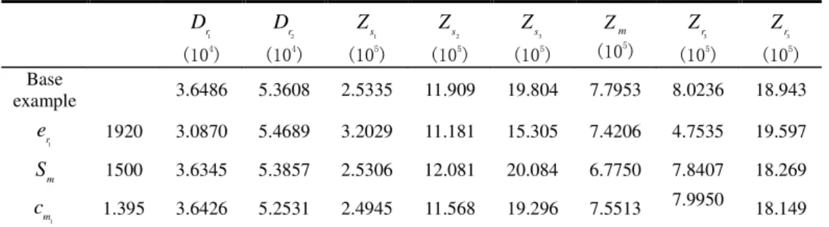
V. NUMERICAL EXAMPLE AND SENSITIVE ANALYSIS
In this section, we present a simple numerical example to demonstrate the applicability of the proposed solution procedure to our game model. We consider a supply chain consisting of three suppliers, one single manufacturer and two retailers. The manufacturer procures three kinds of raw materials from the three suppliers. Then the manufacturer uses them to produce two different products and distributes them to two retailers. The related input parameters for the base example are based on the suggestions from other researchers ([7, 11, 16]). For example, the holding cost per unit final product at any retailer should be higher than the manufacturer’s. The manufacturer’s setup cost should be much larger than any ordering cost. These parameters for the based example are given as:
1 0.01 s
h ,
2 0.008 s
h ,
3 0.002 s
h ,Os1 12, Os223
,
2 13
s
O ,
1 0.93 s
c ,
2 2
s
c ,
3 6 s
c ,
1
0.05
s mr
h ,
2 0.02 s mr
h ,
3 0.04
s
mr
h ,
1 0.5 mp
h ,
2 1 mp
h , cm115,
2 25
m
c , 11 1 s , 12 2 s , 13 3 s , 21 5 s , 22 4 s , 23 2 s
, Sm1000, Om50, P1500000, P2300000,
1 1 r
h , hr22 ,
1 200000 r
A , Ar2 250000 , er11600 , 2 1400
r
e , 1 40
r
O , 2 30
r
O . And the fixed cost for all the
conduct some sensitive analysis on some parameters, including the market related parameter, the production related parameter and the raw material related parameter.
Through the three-level nested Nash game model and the numerical example, some meaningful managerial implications can be drawn:
(1) The increase of market parameter
1
r
e
will reduce the retailer 1’s profit, but benefit the other retailer. When1
r
e
increases, the change of the retailer 1’s demand is more sensitive to the change of his retail price compared with the base example. The retailer 1’s profit can be less reduced by lowering down his retail price. But his market demand cannot be increased, which makes the manufacturer seek for higher profit from other product to fill up the loss deduced by this product / retail market. It is good news to the other product / retailer, because the manufacturer will lower down his wholesale price to stimulate this market demand.
(2) When the manufacturer’s setup cost
S
m increases, themanufacturer’s profit decreases more significantly than the retailers’, while some suppliers’ profits increase. The increase of
S
m makes the manufacturer produce moreproduct with higher profit margin (product 2) and reduce the production of lower profitable product (product 1). The usage of raw materials increases as the change of the manufacturer’s production strategy. At the same time, some suppliers bump up their prices, thus bringing higher profits to them.
(3) The impact of the increase of supplier 1’s raw material cost
1
s
c
on his own profit may not as significant as that on the other suppliers’. The increase of1
s
c
makes the supplier 1 raise his raw material price and result in an increase cost in final products, as well as the decrease in market demands. Hence, the other suppliers will reduce their prices to keep the market and optimize their individual profits. Supplier 1 has the much lower profit margin than other suppliers, so he will not reduce his profit margin. Hence, the supplier 1’s profit decreases least.(4) When the market parameter
1
r
e
, the manufacturer’s setup costS
m, or the supplier’s raw material cost1
s
c
increase, the manufacturer’s setup time interval will be lengthened. A higher1
r
e
or1
s
c
results in the total market demands decrease, as well as a lower inventory consumption rate. The increase ofS
m makes the manufacturer’s cost per production hike up. Hence, the manufacturer has to conduct his production less frequently.VI. CONCLUSION
In this paper, we have considered coordination of pricing and replenishment cycle in a multi-level supply chain composed of multiple suppliers, one single manufacturer and multiple retailers. Sensitive analysis has been conducted on market parameter, production parameter and raw material parameter. The results of the numerical example also show that: (a) when one retailer’s market becomes more sensitive to their price, his profit will be decreased, while the other retailer’s profit will increase; (b) the increase of the
manufacturer’s production setup cost will bring losses to himself and the retailers, but may increase the profits of some suppliers; (c) the increase of raw material cost causes losses to all the supply chain members. Surprisingly, the profit of this raw material’s supplier may not decrease as significant as the other suppliers’; (d) the setup time interval for the manufacture will be lengthened as the increase of the retailer’s price sensitivity, the manufacturer’s setup cost or the supplier’s raw material cost.
However, this paper has the following limitations, which can be extended in the further research. Although this paper considers multiple products and multiple retailers, the competition among them is not covered. Under this competition, the demand of one product / retailer is not only the function of his own price, but also the other products’ / retailers’ prices. Secondly, the suppliers are assumed to be selected and single sourcing strategy is adopted. In fact, either supplier selection or multiple sourcing is an inevitable part of supply chain management. Also, we assume that the production rate is greater than or equal to the demand rate to avoid shortage cost. Without this assumption, the extra cost should be incorporated into the future work.
REFERENCES
[1] Adams, D. 1995. Category management – A marketing concept for
changing times, in: J. Heilbrunn ed. Marketing Encyclopedia: Issues and trends shaping the future.
[2] Boyaci, T., G. Gallego, “Coordinating pricing and inventory
replenishment policies for one wholesaler and one or more geographically dispersed retailers,” International Journal of Production Economics, 77(2), 95-111, 2002.
[3] Curran, T. A., A. Ladd. 2000. SAP/R3 business blueprint:
understanding enterprise supply chain management. Upper Saddle River: Prentice Hall.
[4] Esmaeili, M., Mir-Bahador Aryanezhad, P. Zeephongsekul, “A game
theory approach in seller-buyer supply chain,” European Journal of Operations Research, 191(2), 442-448. 2008.
[5] Huang, Yun, G.Q. Huang, “Game-theoretic coordination of marketing
and inventory policies in a multi-level supply chain,” Lecture Notes in Engineering and Computer Science: Proceedings of The World Congress on Engineering 2010, WCE 2010, 30 June - 2 July, 2010, London, U.K., pp2033-2038.
[6] Jaber, M. Y., S. K. Goyal, “Coordinating a three-level supply chain
with multiple suppliers, a vendor and multiple buyer,” International Journal of Production Economics, 11(6), 95-103, 2008.
[7] Liu, Baoding, “Stackelberg-Nash Equilibrium for multilevel
programming with multiple followers using genetic algorithms,” Computer Math. Application, 36(7), 79-89, 1998.
[8] Lu, L., “A one-vendor multi-buyer integrated inventory model,”
European Journal of Operational Research, 81(2), 312-323, 1995
[9] Moutaz Khouja, “Optimizing inventory decisions in a multi-stage
multi-customer supply chain,” Transportation Research Part E, 39, 193-208, 2003.
[10] Porter M., 1985, Competitive advantage: creating and sustaining
superior performance, New York: The Free Press.1985
[11] Prafulla Joglekar, Madjid Tavana, Jack Rappaport, “A comprehensive
set of Models of intra and inter-organizational coordination for marketing and inventory decisions in a supply chain,” International Journal of Integrated Supply Management, 2006.
[12] Sandoe, K., G. Corbitt, R. Boykin. 2001. Enterprise integration. New
York: John Wiley and Sons.
[13] Viswanathan S., Q. Wang, 2003, Discount pricing decisions in
distribution channels with price-sensitive demand, European Journal of Operational Research, 149, 571-587.
[14] Weng, Z.K, “Channel coordination and quantity discounts,”
Management Science, 41(9), 1509-1522, 1995.
[15] Weng, Z.K, R.T. Wong, “General models for the supplier’s all-unit
quantity discount policy,” Naval Research Logistics, 40(7), 971-991,
1993.
[16] Woo Y. Y., Shu-Lu Hsu, Soushan Wu, “An integrated inventory model
for a single vendor and multiple buyers with ordering cost reduction,”
[17] Yu Yugang, Liang Liang, George Q. Huang, “Leader-follower game in vendor-managed inventory system with limited production capacity
considering wholesale and retail prices,” International Journal of
Logistics: Research and Applications, 9(4), 335-350, 2006.
Table 1. Results for suppliers, manufacturer and retailers under different parameters (a) Product demand and profits for suppliers, manufacturer and retailers
(b) Pricing and replenishment decisions for suppliers, manufacturer and retailers
1 s p
2 s p
3 s p
1
m p
2 m p
3 r p
3 r p
1 s K
2 s K
3 s K
1 r k
2 r
k T
1.77 6.15 15.15 79.37 101.96 102.20 140.28 1 1 2 6 11 0.2691 1.99 5.99 13.58 71.98 100.42 88.09 139.51 1 1 2 6 11 0.2695 1.76 6.20 15.27 79.55 101.61 102.28 140.10 1 1 1 7 14 0.3252
2.23 6.09 15.01 79.44 103.50 102.23 141.05 1 1 2 6 11 0.2707
1 r D (104
) 2 r D (104
)
1 s Z (105
)
2 s Z (105
) 3 s Z (105
)
m Z (105
) 3 r Z (105
) 3 r Z (105
)
Base
example 3.6486 5.3608 2.5335 11.909 19.804 7.7953 8.0236 18.943
1 r
e 1920 3.0870 5.4689 3.2029 11.181 15.305 7.4206 4.7535 19.597
m
S 1500 3.6345 5.3857 2.5306 12.081 20.084 6.7750 7.8407 18.269
1 m
c 1.395 3.6426 5.2531 2.4945 11.568 19.296 7.5513 7.9950 18.149