The Ecological Dynamics of Fecal
Contamination and
Salmonella
Typhi and
Salmonella
Paratyphi A in Municipal
Kathmandu Drinking Water
Abhilasha Karkey1☯, Thibaut Jombart2☯, Alan W. Walker3,4, Corinne N. Thompson5,6,
Andres Torres7, Sabina Dongol1, Nga Tran Vu Thieu5, Duy Pham Thanh5, Dung Tran Thi Ngoc5, Phat Voong Vinh5, Andrew C. Singer8, Julian Parkhill3, Guy Thwaites5,6,
Buddha Basnyat1, Neil Ferguson2, Stephen Baker5,6,9*
1Oxford University Clinical Research Unit, Patan Academy of Health Sciences, Kathmandu, Nepal,2MRC Centre for Outbreak Analysis and Modelling, Department of Infectious Disease Epidemiology, School of Public Health, Imperial College London, London, United Kingdom,3The Wellcome Trust Sanger Institute, Hinxton, Cambridgeshire, United Kingdom,4Microbiology Group, The Rowett Institute of Nutrition and Health, University of Aberdeen, Aberdeen, United Kingdom,5The Hospital for Tropical Diseases, Wellcome Trust Major Overseas Programme, Oxford University Clinical Research Unit, Ho Chi Minh City, Vietnam, 6Centre for Tropical Medicine, Oxford University, Oxford, United Kingdom,7Grupo de Investigación Ciencia e Ingeniería del Agua y el Ambiente, Facultad de Ingeniería, Pontificia Universidad Javeriana, Bogotá, Colombia,8NERC Centre for Ecology and Hydrology, Wallingford, Oxfordshire, United Kingdom, 9The London School of Hygiene and Tropical Medicine, London, United Kingdom
☯These authors contributed equally to this work. *sbaker@oucru.org
Abstract
One of the UN sustainable development goals is to achieve universal access to safe and affordable drinking water by 2030. It is locations like Kathmandu, Nepal, a densely popu-lated city in South Asia with endemic typhoid fever, where this goal is most pertinent. Aiming to understand the public health implications of water quality in Kathmandu we subjected weekly water samples from 10 sources for one year to a range of chemical and bacteriologi-cal analyses. We additionally aimed to detect the etiologibacteriologi-cal agents of typhoid fever and longitudinally assess microbial diversity by 16S rRNA gene surveying. We found that the majority of water sources exhibited chemical and bacterial contamination exceeding WHO guidelines. Further analysis of the chemical and bacterial data indicated site-specific pollu-tion, symptomatic of highly localized fecal contamination. Rainfall was found to be a key driver of this fecal contamination, correlating with nitrates and evidence ofS. Typhi andS. Paratyphi A, for which DNA was detectable in 333 (77%) and 303 (70%) of 432 water sam-ples, respectively. 16S rRNA gene surveying outlined a spectrum of fecal bacteria in the contaminated water, forming complex communities again displaying location-specific tem-poral signatures. Our data signify that the municipal water in Kathmandu is a predominant vehicle for the transmission ofS. Typhi andS. Paratyphi A. This study represents the first extensive spatiotemporal investigation of water pollution in an endemic typhoid fever setting
OPEN ACCESS
Citation:Karkey A, Jombart T, Walker AW, Thompson CN, Torres A, Dongol S, et al. (2016) The Ecological Dynamics of Fecal Contamination and SalmonellaTyphi andSalmonellaParatyphi A in
Municipal Kathmandu Drinking Water. PLoS Negl Trop Dis 10(1): e0004346. doi:10.1371/journal. pntd.0004346
Editor:John A. Crump, University of Otago, NEW ZEALAND
Received:June 29, 2015
Accepted:December 9, 2015
Published:January 6, 2016
Copyright:© 2016 Karkey et al. This is an open access article distributed under the terms of the Creative Commons Attribution License, which permits unrestricted use, distribution, and reproduction in any medium, provided the original author and source are credited.
Data Availability Statement:All relevant data for this study are available within its supporting information files, and the sequence data is available at the European Nucleotide Archive under Study Accession Number ERP004371/Sample Accession number ERS373486.
and implicates highly localized human waste as the major contributor to poor water quality in the Kathmandu Valley.
Author Summary
Aiming to understand the ecology of municipal drinking water and measure the potential exposure to pathogens that cause typhoid fever (SalmonellaTyphi andSalmonella Paraty-phi A) in Kathmandu, Nepal, we collected water samples from 10 water sources weekly for one year and subjected them to comprehensive chemical, bacteriological and molecular analyses. We found that Kathmandu drinking water exhibits longitudinal fecal contamina-tion in excess of WHO guidelines. The chemical composicontamina-tion of water indicated site-spe-cific pollution profiles, which were likely driven by localized contamination with human fecal material. We additionally found thatSalmonellaTyphi andSalmonella Paratyphi A could be detected throughout the year in every water sampling location, but specifically peaked after the monsoons. A microbiota analysis (a method for studying bacterial diver-sity in biological samples) revealed the water to be contaminated by complex populations of fecal bacteria, which again exhibited a unique profile by both location and time. This study shows thatSalmonellaTyphi andSalmonella Paratyphi A can be longitudinally detected in drinking water in Kathmandu and represents the first major investigation of the spatiotemporal dynamics of drinking water pollution in an endemic typhoid setting.
Introduction
Enteric (typhoid) fever is a severe systemic infection and a common cause of community acquired febrile disease in many low-income countries in Asia and Africa [1]. The infection is triggered by the ingestion of the bacteriaSalmonellaTyphi (S. Typhi) andSalmonellaParatyphi A (S. Paratyphi A). BothS. Typhi andS. Paratyphi A are human restricted pathogens (they have no known animal reservoir) and is it acknowledged that they are transmitted through contaminated food and water or via contact with fecal matter from acute or chronically infected individuals [1]. However, the predominant route of infection has never been rigor-ously investigated in an endemic setting outside a conventional case/control study design [2,3].
Typhoid fever is a common infection in Kathmandu (the capital city of Nepal) and our pre-viously generated serological data implies that the local population has longitudinal exposure to both of these endemic pathogens [3,4]. Further studies, generated through investigating the spatiotemporal dynamics of typhoid fever in Kathmandu predicted that bothS. Typhi andS. Paratyphi A are more likely to be transmitted through contaminated water than via human-to-human transmission in this setting [5,6]. Significantly, we found that typhoid fever cases cluster in areas with a high density of urban water sources, which are gravity driven and, therefore, rationally located at lower elevations. The various urban water sources in Kathmandu are most commonly in the form of sunken wells (as found in many urban and rural settings in lower-income countries), piped supplies into large communal holding tanks or the more traditional stone waterspouts (hitis/dhunge dharas) [7]. The iconic stone spouts are common across the Nepalese capital and the water flow into these sacred locations is gravity-dependent (Fig 1a), replenished by rainfall and snowmelt from the surrounding Himalayan Mountains. Natural soft-rock aquifers act as reservoirs for ground water and ultimately the untreated water enters the stone spouts from the aquifers through a series of ancient porous underground channels.
pyrosequencing was provided by the Wellcome Trust (098051). AWW and The Rowett Institute of Nutrition and Health, University of Aberdeen, receive core-funding support from the Scottish Government Rural and Environmental Science and Analysis Service (RESAS). SB is a Sir Henry Dale Fellow, jointly funded by the Wellcome Trust and the Royal Society (100087/Z/12/Z). The funders had no role in study design, data collection and analysis, decision to publish, or preparation of the manuscript.
Competing Interests:The authors have declared
Our previous analysis specifically identified locations around these stone spouts are hotspots forS. Typhi andS. Paratyphi A infections [5,6].
Hypothesizing that the local water, particularly the water accessed via the stone spouts, is a substantial public health risk for typhoid fever and other enteric infections in Kathmandu, we aimed to longitudinally assess bacterial contamination, the chemical composition and the eco-logical dynamics of enteric bacteria in the water supply in this location. To address this hypoth-esis, and focusing on water sources accessed by the local population, weekly water samples were collected over a one-year sampling period from ten locations and subjected to various physical, chemical, microbiological and molecular analyses.
Methods
Water sampling locations
The water sources for this study were the ten most commonly used water sources (identified by questionnaire) lying within a previously identified typhoid fever hotspot in Lalitpur,
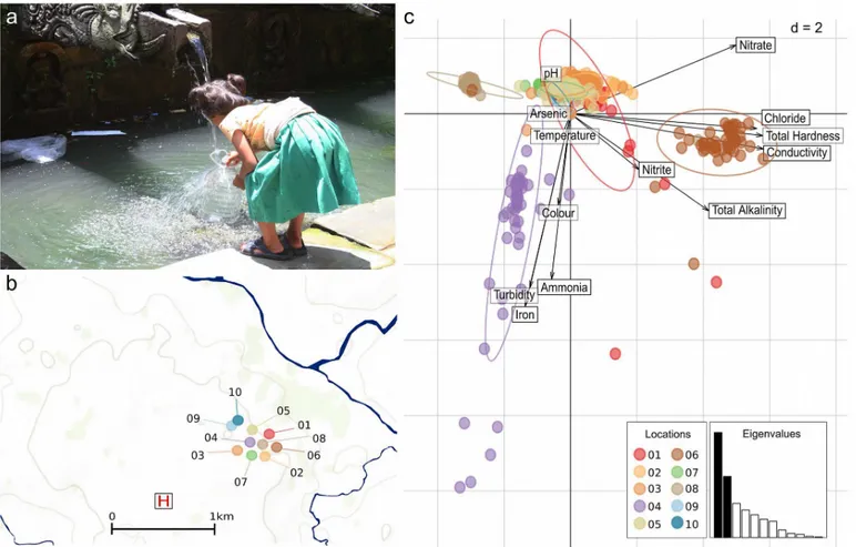
Fig 1. The physical and chemical properties of water from ten sampling locations in Kathmandu, Nepal.a) Photograph of child collecting water from a traditional stone waterspout (dhunge dhara) in Kathmandu. b) A map showing the location of the ten sampling locations in Kathmandu. The locations are color-coded corresponding to other figures and the site of Patan hospital (the healthcare facility for those with typhoid fever) is highlighted by the H symbol. (SeeTable 1and Bakeret al. [6] for more details regarding the sampling locations and the mapped area). c) Scaled principal components analysis of the physical and chemical properties of water samples from the ten sampled locations, showing the first two principal components (PC1-2). Individual water sample are identified by dots colored according to their sampling location (see Fig 1a). Inertia ellipses indicate the overall distribution of each water source. Labeled arrows indicate the relative contributions of the variables to the principal components, with longer arrows reflecting larger contributions. The screeplot of eigenvalues (inset) indicates the amount of variation contained in the different principal components, with PC1 and PC2 indicated in black.
Kathmandu [6]. The selected locations were GPS located using an eTrex legend (Garmin) and consisted of five stone spouts, three sunken wells and two piped supplies. The location of these water sources are shown inFig 1band described in detail inTable 1. Daily rainfall data from Kathmandu Airport was provided by the Nepalese Department of Hydrology and Mete-orology (http://www.dhm.gov.np/) and aggregated into weeks for the purposes of the analysis presented here.
Collection of water samples for analysis
Water was collected (when permitted by water flow), from all of the 10 locations once per week over one year from May 2009 to April 2010. From each of the sources mid-flow water samples were collected in two sterile bottles in volumes of 1 L and 500 ml. From the stone spouts and the piped supply, the stopper was aseptically removed and free flowing water was allowed to flow directly into the sterile bottle. For wells, a sterilized steel bucket (bleached and washed with autoclaved water prior to use) was lowered into the well until it was partially submerged, the bucket was then removed and the water was poured into the bottles. All the bottles were labeled with the source code, date and time of collection of the samples. After recording the water temperature the bottles were transported to the laboratory at ambient temperature and were processed within one hour for physical, chemical and microbiological analysis.
Physical and chemical analysis of water samples
The Kathmandu Water Engineering Laboratory (
http://www.sodhpuch.com/water-engineering-training-centre-p.) performed all chemical and physical analyses following their standard operating procedures for international water quality. The measured variables were pH (Hanna pH meter, calibrated with pH4, pH7 and pH9 buffers), temperature (Hanna digital thermometer with probe), conductivity (Hanna conductivity meter), color (Perkin Elmer’s LAMDA 650 UV spectrophotometer at 270 nm) turbidity (NEPHELOstar Plus nephlometer), hardness (EDTA titration), total alkalinity as CaCO3(methyl orange), chloride (argentometric
titration), ammonia (nesslerisation), total nitrate (Perkin Elmer’s LAMBDA 650 UV spectro-photometer at 275 nm), total nitrite (Perkin Elmer’s LAMDA 650 UV spectrophotometer at 275 nm), and trace elements and heavy metals (Atomic Absorption Spectrophotometric (AAS) method). All variables were recorded on the day of sampling and compared to WHO guide-lines for water quality [8].
Most Probable Number (MPN) method for measuring thermotolerant
coliforms
A modified most probable number (MPN) method was used to assess the microbiological qual-ity of the water, specifically coliform contamination [9,10]. Briefly, five ten-fold serial dilutions were made from each water sample by inoculating 1 ml of undiluted water sample into 9 ml of MacConkey broth (Oxoid, UK). This was continued until a dilution of 1 x 10⁻⁵. A total of 30
Direct and enrichment plating for enteric bacteria in water
To detect the presence of enteric bacteria with pathogenic potential (e.g.Salmonellae,Shigellae,
Vibrionaceae, andE.coli) 10, 20, 50, 100 and 500μl of undiluted water was directly plated onto
Xylose lysine deoxycholate (XLD) and MacConkey agar plates. The plates were incubated at 37°C overnight and then observed for growth. To increase the likelihood of culturing Salmonel-laeandShigellae, 100 ml of undiluted water was filtered through a membrane filter with a pore size 0.45μm (Whatman, GE Life Sciences, PA, USA) using a sterile syringe. The filter paper
was removed using sterile forceps and placed in 90 ml of typtic soya broth (Oxoid, UK). The soya broth bottles were agitated using a vortex to displace the organisms on the membrane and incubated for 18 hours at 37°C. After overnight incubation 1 ml of the pre-enrichment culture was transferred to 10 ml of selenite broth. Further, 1 ml of the pre-enrichment culture was transferred to 10 ml of Rappaport-Vassiliadis Broth (RVB). The incubated overnight broth was then plated onto XLD and MacConkey agar plates. The plates were incubated overnight at 37°C and then observed for growth. For the detection ofVibrionaceae, 1 ml of the undiluted water sample was diluted in 9 ml of alkaline peptone water. The suspension was then incubated overnight at 37°C and then plated on to MacConkey, XLD and thiosulphate-citrate-bile salts sucrose (TCBS) agar.
Bacterial identification
The colony morphologies including the form, size, surface appearance, texture, color, elevation and margin of all individual colonies were recorded from MacConkey and XLD plates. Of spe-cial interest were colonies that were circular, with an entire margin and slightly raised elevation that were non-lactose fermenting on both plates, with or without the production of hydrogen sulphide on the XLD plate. Individual colonies with the aforementioned characteristics were isolated and plated on nutrient agar and incubated at 37°C for 24 hours. Isolated colonies
Table 1. Water sampling locations in this study.
Location Source type
Latitude Longitude Depth to water (m)
Source Treatment Additional protection Samples collected/weeks 16S rRNA gene analysis 1 Stone spout N 27° 40.482 E 85° 19.693
Ground level Shallow aquifer
Untreated None 40/53 No
2 Stone spout N 27° 40.461 E 85° 19.693
Ground level Shallow aquifer
Untreated None 38/53 Yes
3 Stone
spout
N 27° 40.426
E 85°19.51 Ground level Shallow aquifer
Untreated None 51/53 No
4 Sunken well N 27° 40.454 E 85° 19.665 8.4 Shallow aquifer
Untreated Mesh covered 51/53 No
5 Sunken well N 27° 40.503 E 85° 19.660 7.1 Shallow aquifer
Untreated Mesh covered 50/53 Yes
6 Sunken well N 27° 40.545 E 85° 19.719 8.1 Shallow aquifer
Untreated Mesh covered 50/53 No
7 Piped supply N 27° 40.422 E 85° 19.645
Ground level Delivery truck Irregular chlorination Locked container 51/53 No 8 Piped supply N 27° 40.457 E 85° 19.698
Ground level Delivery truck Irregular chlorination Locked container 50/53 No 9 Stone spout N 27° 40.607 E 085° 19.540
Ground level Shallow aquifer
Untreated None 21/53 No
10 Stone spout N 27° 40.607 E 085° 19.540
Ground level Shallow aquifer
Untreated None 30/53 No
obtained on the nutrient agar plates were then subject to API20E testing to identify Enterobac-teriaceaeand other non-fastidious Gram-negative rods.
Total DNA extraction from water samples
Total DNA from all water samples was extracted using the Metagenomic DNA Isolation Kit for Water (Epicentre Biotechnologies, WI, USA). Water samples were centrifuged at 1,000 rpm (Hettich Zentrifugen, EBA 21, Germany) for 5 minutes to remove large debris and then decanted into sterile containers. After centrifugation, 100 ml of the centrifuged water was fil-tered through a pre-sterilized filter with a pore size of 0.45μm (Whatman, GE Life Sciences,
PA, USA). Using sterile forceps and scissors the membrane was removed from the filter appa-ratus and cut into four pieces. The cut filters were then placed in a 50 ml sterile conical tube with the upper surface of the filter facing inwards. One milliliter of filter wash buffer containing 0.2% Tween-20 was added to the filter pieces in the tubes to remove organisms on the filter sur-face. The tube was agitated at high speed for approximately 2 minutes with intermittent breaks. The cell suspension was transferred to a clean micro-centrifuge tube and centrifuged at 14,000 X g (Thermo Fischer Scientific, IEC Micro CL17, Germany) for 2 minutes to pellet the cells. The supernatant was discarded. The cell pellet was re-suspended in 300μl of TE buffer, and
2μl of ready-lyse lysozyme solution and 1μl of RNAse A were added and mixed thoroughly.
The tube was incubated at 37°C for 30 minutes and then 300μl of 2 X meta-lysis solutions and
1μl of Proteinase K were added to the tube and thoroughly mixed by vortexing. To ensure that
all the solution was at the bottom of the tube, the tube was pulse centrifuged. The tubes were then incubated at 65°C for 15 minutes. The solution was cooled to ambient temperature and placed on ice for 5 minutes. 350μl of MPC protein precipitation reagent was added to the tube
and mixed thoroughly by vortexing vigorously for 10 seconds. The debris was pelleted by cen-trifugation for 10 minutes at 14,000 X g (Thermo Fischer Scientific, IEC Micro CL17, Ger-many) at 4°C. The supernatant was transferred to a clean micro-centrifuge tube and the pellet was discarded. To the supernatant, 570μl of isopropanol was added and mixed by inverting
the tube multiple times. The DNA was pelleted by centrifugation for 10 minutes at 14,000 X g (Thermo Fischer Scientific, IEC Micro CL17, Germany) at 4°C. The isopropanol was removed and the sample was briefly pulse centrifuged and any residual liquid was removed without dis-turbing the pellet. To the pellet 500μl of 70% ethanol was added without disturbing the pellet.
The tube was then centrifuged for 10 minutes at 14000 X g (Thermo Fischer Scientific, IEC Micro CL17, Germany) at 4°C. Ethanol was removed without dislodging the DNA pellet and the sample was briefly pulse centrifuged and any residual fluid was removed without disturbing the pellet. The pellet was then air dried for 8 minutes at ambient temperature before being resuspended in 100μl of nucleic acid free sterile water (Epicentre Biotechnologies, WI, USA).
Real-time polymerase chain reaction to detect
S
. Typhi and
S
. Paratyphi
A in water samples
Quantitative Real-time PCR was performed on all extracted DNA to detect DNA sequences specific forS. Typhi andS. Paratyphi A as previously described [11]. Primer and probe sequences were as follows;S. Typhi; ST-Frt 5' CGCGAAGTCAGAGTCGACATAG 3', ST-Rrt 5' AAGACCTCAACGCCGATCAC 3', ST- Probe 5' FAM-CATTTGTTCTGGAGCAGGCT GACGG-TAMRA 3';S. Paratyphi A; Frt 5'ACGATGATGACTGATTTATCGAAC 3', Pa-Rrt 5' TGAAAAGATATCTCTCAGAGCTGG 3', Pa-Probe 5' Cy5-CCCATACAATTTCA TTCTTATTGAGAATGCGC-BHQ5 3'. Briefly, 5μl of environmental DNA extractions (as
above from 100 ml of water and resuspended in 100μl of nucleic acid free sterile water)
Quantification was performed using standard curves where plasmid DNA carrying the target sequences were diluted in 10-fold serial dilutions ranging from 100to 105plasmid copies perμl; standard curves for assessingS. Typhi andS. Paratyphi A copy number were
con-structed by plotting theCtvalue against the plasmid DNA copy number.
16S rRNA gene amplification and sequencing
For the 16S rRNA gene surveying, variable regions 3 to 5 (V3–V5) of the 16S rRNA gene were PCR amplified from the water DNA extractions. The primers used were as described previously [12], seeS1 Tablefor the full barcode and primer sequences (30 nucleotides for 454 adaptor, 12 nucleotides for unique recognition (tag) and 18 nucleotides to amplify the specific V3–V5 region) used for each sample in the present study. The conditions of PCR were as follows: 1U of AccuPrime Taq DNA Polymerase High Fidelity (Invitrogen, Carlsbad, CA USA), 200 mM of forward and reverse primer, 2μl of template environmental DNA in a 20μl reaction. The
reaction was cycled for 1 x 94°C for 2 minutes, and then 20x (94°C for 30 seconds, 53°C for 30 seconds and 68°C for 2 minutes). Each sample was PCR amplified on four occasions, the result-ing amplicons were pooled and then ethanol precipitated before resuspension in 20μl of TE.
The 16S rRNA gene amplicons were shipped to The Wellcome Trust Sanger Institute and pooled together into an equimolar mastermix, as measured by a Qubit fluorometer (Invitrogen, Carlsbad, CA, USA), prior to sequencing on a GS FLX Titanium 454 machine (Roche Diagnos-tics, Oakland, CA USA) using the Lib-L kit. The resulting sequence data is available at the European Nucleotide Archive under Study Accession Number ERP004371/Sample Accession number ERS373486. Sequence data was processed using the mothur software package (http:// www.mothur.org/), following a previously described protocol [12]. This removed poor quality reads, and generated taxonomic classifications for each Operational Taxonomic Unit (OTU). Following these filtering steps 326,155 sequences remained (range of 1 to 7,396 sequences per sample).
Statistical analysis of bacterial contamination data
We first tested for geographic differences in bacterial assays, using the non-parametric MAN-OVA implemented in the packageade4 [13] for the R software suite [14]. 9,999 random per-mutations of the data were used to assess statistical significance of Pillai’s statistic [15] and compute the associatedp-value. After ruling out the presence of geographic differences between samples, data were aggregated across locations by computing average weekly profiles, from which temporal trends were more straightforward to investigate. As bacterial assays may each capture different aspects of water contamination, these data were subjected to a centered Principal Component Analysis (PCA) [13], which we used to derive a latent variable (the first principal component, PC1) as correlated as possible to all the different assays [16] and there-fore reflecting the extent of bacterial contamination. PCA is ideally suited to derive synthetic variables, which capture the essential trends of variation in quantitative or binary data, and is thus readily applicable to water quality data including physical chemical properties, bacterial assays and meta-genomic variation.
Statistical analysis of chemical pollution data
As for bacterial assays, the various chemical properties measured captured potentially different aspects of water pollution. PCA was used to identify the main trends of variation amongst water samples [18,19]. Because measurements were made using different units and had inher-ently different scales of variation, a centered and scaled PCA was used [20]. Missing data were replaced by the average of the corresponding variables, as is customary in PCA [20]. Results of this first PCA were driven by an outlier, which turned out to be a sample of exceptionally poor water quality. In such cases, because PCA finds linear combinations of variables with maxi-mum variance, the presence of an outlier may conceal other interesting structures [20]. As a consequence, this sample was removed in a second PCA, the results of which are shown inFig 2. Differences in water chemistry of the water sources were tested using the same MANOVA procedure used in bacterial assays analysis.
Spatiotemporal dynamics of bacterial composition from 16S rRNA gene
data
16S rRNA gene survey data consisting of 93 samples and 11,212 OTUs were first transformed into compositional data [21], so that each sample was transformed into a composition of OTUs frequencies summing to 1. This transformation ensures that further analysis will only reflect differences in taxa composition, and not in absolute quantities of sequenced DNA. The Gini-Simpson index was computed for every sample as1P
ip2i wherepiis the relative
fre-quency of OTUiin the sample. A centered PCA was used to analyze the metagenomic profiles, retaining thefirstfive principal axes as they expressed most of the structured variation in the data (Fig 3a). The proportion of the total variation represented by thejthprincipal axis was computed asλ
j/∑jλj(Fig 3b). The contribution of an OTUito a principal axisUdefined by a
vector of loadings [u1,u2,. . .,u11,212] was computed asui2, which is justified by the fact thatU
has a norm of 1 (thus_U_2=∑iui2= 1). The OTUs contributing most to the retained
princi-pal axes were defined as OTUs with contributions greater than a given threshold (Fig 3c). Dif-ferent sets of OTUs were defined using thresholds of 1%, 2%, 5%, 10%, 20%, 30%, 40%, and 50%, which resulted in retention of between 4 and 14 OTUs. A threshold of 10% was retained as it allowed for conserving essentially all of the variation of the 7 principal axes with only 10 OTUs, which still represented 80% of the total variation in the data.
Discriminant Analysis of Principal Components (DAPC, [22,23]) was applied to the 16S rRNA gene data to identify combinations of OTUs that differed most between stone spouts and well. While originally developed for genetic markers data, this method has since been applied to various other types of data, including 16S rRNA (e.g. [24,25]). Cross-validation was used to assess the optimal number of PCA axes to retain in the preliminary dimension-reduc-tion step, using 100 independent replicates for each number of retained PCA axes and 70% of the samples as training set. The same analyses were repeated to investigate possible differences across the three locations.
Results and Discussion
The chemical and physical properties of Kathmandu drinking water
but notably, only nitrate levels and turbidity consistently exceeded WHO recommendations in all locations. These finding, with respect to nitrate were broadly consistent with previous single time point observations in this location [26,27]. Further investigation identified significant differences in the chemical profiles of the water from the various locations (non-parametric MANOVA:Λ
pillai= 0.250,p= 1×10
−4with 9,999 permutations). These disparities in chemical
compositions could be summarized using a PCA, with water from two of the sunken wells (locations 4 and 6 (Table 1andFig 1b)) forming distinct clusters with independent chemical signatures (Fig 1c). These profiles were characterized by consistently high concentrations of iron and ammonia and greater turbidity at location 4 and greater conductivity, hardness, chlo-rides and nitrates at location 6 (Fig 1c). Distinctively, one of the piped water supplies (location 8) had consistently lower chemical contamination indices than all other sources (Fig 1cand
Table 2). The differences in chemical composition between locations, confirmed by pairwise comparisons between the sampling locations (Wilcoxon rank test, allp-values<0.05 with
Fig 2. The quantification of coliforms and DNA fromSalmonellaserovars Typhi and Paratyphi A in water samples from ten locations in
Kathmandu, Nepal.a) Boxplots of the MPN counts (log10 CFU/ml) aggregated by water sources type (SS, stone spout; SW, sunken well; PS, piped supply) and within each individual location (numbered on x-axis). Boxes and horizontal lines represent the interquartile ranges and medians, respectively and whiskers represent 90% of data range. The median MPN measurements in water from stone spouts; sunken wells and piped supplies were significantly different; as determined by Kruskal Wallis test (p<0.001; shown by the asterisk). b) Scatterplots showing the number of copies ofS. Typhi (red circles) andS.
Paratyphi A (blue circles) gene targets calculated to be in each water sample (by realtime PCR amplification and quantification using a standard curve) against the week of sampling. The red and blue shaded lines show the best fit through time of gene copy quantification trends forS. Typhi andS. Paratyphi A, respectively. c) Principal components analysis of the weekly presence/absence profiles ofS. Typhi andS. Paratyphi A gene targets in water samples, shaded by weekly rainfall (see key). Time is represented on the x-axis. The first principal component, representing fluctuations inS. Typhi andS. Paratyphi A DNA relative abundance, is plotted on the y-axis.
Bonferroni correction), suggest water mineralization and implicate contaminants such as vehi-cle exhaust gases [28,29] and poor waste handling systems as the key drivers of poor water quality in these locations [30].
Of the different chemical pollutants observed in Kathmandu drinking water, the sustained contamination of water by nitrites and nitrates was the most alarming. Nitrites and nitrates can be introduced into the water through a range of processes including surface water infiltra-tion, industrial polluinfiltra-tion, agricultural fertilizer run-off and the leakage of sewerage systems [26,31]. Sustained exposure to nitrates can lead to a range of non-communicable diseases including methemoglobinemia, gastrointestinal cancer, bladder and ovarian cancers, and may expedite type II diabetes, thyroid hypertrophy and respiratory tract infections [32]. Nitrate
Fig 3. 16S rRNA gene surveying of gastrointestinal bacterial taxa found in stone spout and well water samples in Kathmandu, Nepal.a) Screeplot showing the eigenvalues of the PCA of 16S rRNA gene data, with retained axes in blue corresponding to 80% of the variation in 519 identified OTUs from fecal bacterial families (Bacteroidaceae,Clostridiaceae,Enterobacteriaceae,Erysipelotrichaceae,Lachnospiraceae,Lactobacillaceae,Prevotellaceae, RuminococcaceaeandVeillonellaceae) identified in 93 water samples from location 2 (stone spout) and location 5 (sunken well). The main graph only represents the first 30 eigenvalues (full graph provided in inset). b) Diversity represented by the OTUs with large contributions to the retained PCA axes. PCA axes are represented on the x-axis, with a width proportional to the corresponding diversity (eigenvalue). The y-axis represents the amount of diversity retained by retaining only OTUs with contributions of at least 1% (6 taxa), 5% (5 taxa), 50% (4 taxa) or 75% (2 taxa), indicated by differing shades of blue. The total surface of a given color is proportional to the fraction of the total diversity represented by this set of taxa. The red dashed line identifies the set of 6 retained taxa plotted in Fig 3c, representing 76% of the total variation in the entire data. c) OTU composition of the water samples, showing the relative frequencies of the six most structuring fecal bacterial taxa identified in Fig 3b (Enterobacteriaceae(OTUs 00024, 00185 and 01479),Bacteroidaceae (OTU00979),Clostridiaceae(OTU00263), andPrevotellaceae(OTU 2149)). Their relative abundance (y-axis) is represented through time in location 2 (stone spout) and location 5 (sunken well), the two locations with the greatest estimated coliform contamination by MPN. Empty bars correspond to missing or failed samples. d) A Discriminant Analysis of Principal Components (DAPC) of the 16S rRNA gene identifying combinations of the 519 gastrointestinal OTUs differing the most between the stone spout (blue) and the sunken well (red). The OTUs exhibiting the greatest variation between these locations were OTU00263;Clostridium, OTU00185;Enterobacteriaceae, OTU00979;Bacteroidesand OTU00024,Enterobacteriaceae).
excess is also a notable marker of fecal contamination, and we found nitrites and nitrates corre-lated positively with coliform concentration (see below) and weekly rainfall (p<0.001;
Spear-man’s rho). Consistently, the concentration of chloride, again a marker of sewage and manure contamination [33], also increased with the onset of seasonal rainfall (p<0.001; Spearman’s
rho). More generally, several other chemical properties were also associated with weekly rain-fall; positive correlations were observed for rainfall against turbidity, ammonia and hardness (Spearman’s rho,p-values<0.05 in six locations), and negative correlations were observed
with rainfall against pH and alkalinity (Spearman’s rho,p-values<0.05 in four locations).
Taken together, these results suggest that chemical pollution of drinking water in this setting is likely driven by a combination of rainfall runoff and localized contamination with human fecal waste.
Water contamination with coliforms and
Salmonella
serovars Typhi and
Paratyphi A
To determine the extent of potential fecal contamination in the water samples, we estimated the concentration of fecal indicator thermotolerant coliforms using the minimal probable number (MPN) method. The WHO guidelines state that no water directly intended for drink-ing, or in the distribution system should contain thermotolerant coliforms (in a 100ml sample) [8]. We found that majority of the cultured water samples were contaminated with thermoto-lerant coliforms, suggesting that all the sampled water sources are prone to fecal contamination (Table 2). The concentrations of cultured coliforms across the samples ranged from 0.1 to 2.5 x 10⁸CFU/100 ml, these figures are again largely consistent with prior investigations of drinking
Table 2. Summary of the chemical and bacterial contamination of the water sampling locations.
Source Turbidity (NTU) Chloride (mg/L) Ammonia (mg/L) Iron (mg/L) Nitrite (mg/L as NaNO2)
Nitrate (mg/L as NaNO2)
MPN CFU/ 100ml
S. Paratyphi PCR positive (%)
S. Typhi PCR positive (%)
WHO* 0.5 250 1.5 0.3 3 50 0 -
-1 0.5 (0.5, 2) 90.1 (82.2, 112)
0.2 (0.1, 0.4) 0.1 (0, 0.2) 0.04 (0.01, 0.15) 112.9 (98.3, 116.8) 33 (5, 3850)
25/40 (63) 30/40 (75)
2 0.5 (0.5, 1) 109.9 (89.1, 129.7) 0.2 (0.1, 0.33) 0.1 (0, 0.2) 0.02 (0.01, 0.06) 136.2 (119.6, 157.1) 1300 (207, 16750)
28/38 (74) 31/38 (82)
3 0.5 (0.5, 0.5)
83.2 (78.2, 88.1)
0.1 (0.1, 0.1) 0.1 (0, 0.2)
0.01 (0.01, 0.01)
142.7 (135.3, 158.5)
2 (1, 87) 38/51 (75) 40/51 (78)
4 58 (24.5, 115) 57.4 (55.4, 59.4) 10.5 (9.8, 11.2) 11.3 (8.7. 15.1) 0.06 (0.03, 0.13)
3.3 (1.25. 7.6) 1 (1, 2) 36/51 (71) 42/51 (82)
5 4 (2, 7.8) 87.1 (82.4, 94.1)
0.2 (0.1, 0.3) 0.2 (0.1, 0.3) 0.02 (0.01, 0.05) 117.7 (107.3, 127.2) 182 (6, 3025)
33/50 (66) 41/50 (82)
6 3 (2, 4) 169.8 (158.9, 174.6)
1.6 (0.9, 3.2) 0.12 (0.1, 0.5) 0.34 (0.19, 0.57) 191.1 (157.1, 204.5) 137 (7, 1700)
37/50 (74) 38/50 (76)
7 0.5 (0.5, 1) 83.2 (79.7, 90.1)
0.2 (0.1, 0.3) 0.01 (0, 0.2)
0.01 (0.01, 0.02)
93.3 (86.5, 106.0)
14 (2, 745) 39/51 (76) 43/51 (84)
8 2 (1, 2) 10 (9.9, 10.9) 0.1 (0, 0.2) 0.1 (0.1, 0.2)
0.01 (0.01, 0.01)
1.7 (1.6, 1.9) 1 (0, 1) 33/50 (66) 36/50 (72)
9 0.5 (0.5, 0.8)
66.3 (65.3, 68.3)
0.1 (0.1, 0.2) 0.01 (0, 0.2)
0.07 (0.05, 0.07)
94.1 (90.7, 96.3)
34 (7, 460) 15/21 (71) 13/21 (62)
10 0.5 (0.5, 0.6)
65.8 (64.1, 69.3)
0.1 (0, 0.2) 0.1 (0, 0.2) 0.02 (0.02, 0.05) 90.3 (82.4, 93) 31 (6, 2275)
19/30 (63) 19/30 (63)
*According to WHO guidelines [8], Data shown in medians and interquartile ranges unless described otherwise.
water quality in this setting [8,26,31]. The water from the stone spouts (locations 1, 2, 3, 9 and 10 (Table 1) had higher coliform concentrations (median 94 CFU/100 ml; IQR: 4 to 1.6 x 10⁴) than that from the sunken wells (locations 4, 5, 6) (median 8 CFU/100 ml; IQR: 1 to 7.9 x 10⁴) and from the piped supplies (locations 7, 8) (Median 2 CFU/100 ml; IQR: 1 to 170) (p<0.001;
Kruskal Wallis) (Fig 2a). The highest coliform concentrations across the sampled water sources were in the months of June, July and August and, similar to the chemical contamination, posi-tively correlated with the period of increased weekly rainfall (Spearman’s rho=0.27,p<0.001).
The water sampled from source 2 (stone spout) consistently had the highest level of coliform contamination (median coliform concentration; 1.3 x 10⁴CFU/100 ml; IQR: 200 to 1.68 x 10⁵) and had the highest single coliform count of 2.5 x 10⁸CFU/100 ml in August.
The alarming levels of coliform and chemical contamination highlight that water quality is a major public health issue in Kathmandu. The detection of thermotolerant coliforms is not suitable for the identification of specific waterborne pathogens, but is used as a general measure of bacterial contamination [34]. To address this methodological limitation, we concurrently performed membrane filtration and microbiological enrichment for a range of pathogenic bac-terial species classified as high risk by the WHO, includingSalmonella,Shigella,Vibrionaceae
andE.coli[8]. Overgrowth on plates diminished the ability to accurately quantify these organ-isms but we repeatedly cultured and identified a wide range of organorgan-isms with pathogenic potential to humans includingVibrio cholerae01,Shigella dysenteriaetype-1,Pseudomonas
spp., andPlesiomonas shigelloides(S2 Table). We additionally isolated multipleSalmonellaspp. in the water through supplementary enrichment, yet, after serotyping, none were identified as
S. Typhi orS. Paratyphi A.
The lack of confirmative cultures forS. Typhi orS. Paratyphi A is not uncommon given pre-vious efforts to culture these pathogens from water.S. Typhi has been cultured from environ-mental samples previously [35], but is notoriously difficult to isolate from water in endemic locations. It has been suggested thatS. Typhi is often present and viable, but in a non-cultur-able state [36]. To address this limitation we extracted and purified total nucleic acid from each of the water samples after filtration and performed appropriately controlled quantitative real-time PCR on all samples for chromosomal targets specific forS. Typhi andS. Paratyphi A. We found that 333 (77%) and 303 (70%) of 432 DNA extractions from the eater samples were PCR amplification positive forS. Typhi andS. Paratyphi A, respectively (Fig 2b), with 266/432 (62%) samples being PCR amplification positive for both. To confirm that the PCR amplicons wereS. Typhi andS. Paratyphi A, a random cross section of 96 (48 for each serovar) PCR amplicons were successfully cloned, sequenced and confirmed to originate from eitherS. Typhi orS. Paratyphi A. Further, through inference from standard curve, we identified a significant difference between the number of copies/reaction betweenS. Typhi (median 208 copies/reac-tion; IQR: 72 to 603) andS. Paratyphi A (median 11 copies/reaction; IQR: 4.6 to 28), corre-sponding with inferred significantly different medians of 4,200 and 2,200 copies/100 ml, respectively (p<0.001; Kruskal Wallis) (Fig 2b).
The presence ofS. Typhi andS. Paratyphi A DNA in the water samples did not differ signif-icantly across locations (non-parametric MANOVA:Λpillai= 0.020,p= 0.66 with 9,999
season (May–October) (Fig 2c). A simple seasonal model of PC1 (using a spline of the collec-tion dates with five breakpoints) showed that this temporal trend was a significantly better fit than a model where PC1 was constant over time (ANOVA:F= 4.2184,p= 0.0034). Notably, the increased presence ofS. Typhi andS. Paratyphi A in the water samples displayed a substan-tial temporal lag, with PC1 reaching a peak between one to two months after the end of the monsoon rains (Fig 2c). This delay may reflect the time taken for the organisms to reach the water outlet from the source of contamination or a concentration effect reflecting lower ground water levels in drier periods. We speculate that a leaking sewerage system and fluctuations in the pressure in the water supply pipes (negative pressure in the pipe results in an influx of sew-age into the water pipe) are a likely source of this contamination.
16S rRNA gene surveying
While the trend of contamination byS. Typhi andS. Paratyphi A was similar across all sampled locations, these organisms likely represent a microscopic fraction of the diverse communities of microorganisms transiting through these water sources [37]. Assessing these complex microbial communities is relevant for investigating the extent of contaminating organisms present in these water sources and also aids tracing the likely sources of bacterial contamina-tion. (i.e. soil and/or fecal waste). 16S rRNA gene surveying provides a suitably broad approach in conducting this type of investigation [38]. Therefore, the longitudinal structures of the bacte-rial communities in the two water sources with the greatest coliform concentrations (locations 2 and 5) were compared by 16S rRNA gene amplification and pyrosequencing (data available inS2 Dataset) [12]. The resulting 16S rRNA gene data showed that the bacterial communities in 93 tested water samples were composed of 11,212 OTUs, more than half of which were observed only once (S1 Fig). The bacterial diversity, as measured by Gini-Simpson’s index [39], was high in all analyzed samples (S2 Fig). We observed an increase in the average number of taxa found during the dry season (S3 Fig), suggesting that low rainfall induces a concentration effect and that exposure to a wider range of taxa likely increases during this period.
For a more comprehensive analysis, we investigated the bacterial diversity using a PCA of the 16S rRNA gene survey data transformed into OTU frequency profiles. This analysis showed that>80% of the variation amongst the analyzed samples could be summarized in seven
dimensions, each representing a different assemblage of the detected OTUs (S4 Fig). Closer examination of the relative contributions of OTUs to each axis revealed that nearly identical principal components could be obtained through a combination of the 10 most common OTUs, which belonged to the generaAcinetobacter(OTUs 00001 and 0019),Acidovorax
(OTU00011),Comamonas(OTU00025),Flavobacterium(OTU00042),Bacillus(OTUs 00503 and 00155),Chryseobacterium(OTU00208),Staphylococcus(OTU00436) andBrevundimonas
(OTU00707) (S4 Fig).
The ten most commonly detected OTUs were comprised of bacterial genera that are typi-cally found in the environment, and most are not recognized as enteric organisms. While many of these genera are known aquatic organisms, there is some overlap with genera that have recently been demonstrated to originate from sample preparation procedures [40]. To address this limitation, we specifically focused on the relative contributions of nine bacterial families that are common constituents of the gastrointestinal tract of mammals ( Bacteroida-ceae,Clostridiaceae,Enterobacteriaceae,Erysipelotrichaceae,Lachnospiraceae,Lactobacillaceae,
01479),Bacteroidaceae(OTU00979),Clostridiaceae(OTU00263), andPrevotellaceae(OTU 2149) (Fig 3c). We additionally found that the OTU composition was not random, and varied substantially between the sunken well and the stone spout. A DAPC analysis of the 16S rRNA gene data was used to identify combinations of the 519 gastrointestinal OTUs showing the greatest difference between the well (location 5) and the stone spout (location 2). The corre-sponding DAPC was able to recover the type of water source of the samples (based on their OTU composition) in 81% of cases (Fig 3c). The OTUs exhibiting the greatest variation (OTU00263;Clostridium, OTU00185;Enterobacteriaceae, OTU00979;Bacteroidesand OTU00024;Enterobacteriaceae) were additionally four of the six principal fecal OTUs driving the temporal trends (Fig 3d). These results suggest the existence of local ecological factors, such as proximal sewage pipes, strongly affect the composition of bacterial communities in different types of water sources.
The impact of contaminated water on the populous of Kathmandu
The current daily demand for water in Kathmandu is estimated to be 200,000 m3/d, but is unable to be met by municipal supplies, resulting in deficits of 70,000 to 115,000 m3/d in the wet and dry seasons, respectively [26]. This water deficit means that drinking water distribu-tion lines operate at low pressure as compared to the overused sewage pipes that are often co-located. This pressure differential between sewage and drinking water lines, their relative prox-imity and poor state of repair accounts for the ingress of sewage into drinking water lines and an overall deterioration in their quality and safety. Furthermore, the cost associated with municipal water has led to an upsurge in the use of stone spouts in the middle and low-income residents of Kathmandu. The users of stone spouts now represent>20% of the water usage in
Kathmandu [26]. Bacterial contamination has previously been shown to be higher in stone spouts than sunken wells than piped supplies in Kathmandu, with similar trends seen with nitrate contamination [26]. Our data confirm these associations and for the first time we show seasonal variations in fecal contamination, chemical pollutants and, vitally, exposure to bothS. Typhi andS. Paratyphi A. We suggest that stone spouts are the most contaminated type of water source in this location as they are maximally exposed to potentially contaminating sources of human sewage. Further, the shallow aquifers supplying the stone spouts are likely more contaminated than deep aquifers, as they are, again, closer to the sources of potential contamination.
Our work shows that Kathmandu drinking water exhibits year round fecal contamination and is far from compliant with World Health Organization (WHO) standards [8] and it will be challenge to meet the United Nations sustainable development goal six (http://www.un.org/ sustainabledevelopment/water-and-sanitation/#). It has been known for>100 years that the
pipes, urban development, poor sanitation) are likely to be common in other typhoid endemic settings in Asia and beyond.
In conclusion, our work shows that municipal water in the capital city of Nepal exhibits dence of substantial bacterial and chemical contamination. Further, we additionally show evi-dence of longitudinal contamination of bothS. Typhi andS. Paratyphi A, demonstrating the impact of human fecal contamination and outlining that both these organisms are being con-tinually transmitted through these water supply systems. Future research should focus on investigating the main routes of these bacterial and chemical pollutants into this water supply system. Further, the ability to culture and genotype organisms from the environment and human infection would close the circle on the role of the water delivery systems in urban set-tings for the transmission of typhoid fever. Nepal is amongst the poorest countries in Asia (GDP per capita of USD 703 in 2013 [43]) and substantial investment is required to improve the capacity and quality of the water supply in addition to the sewage handling systems in Kathmandu. As a rapid improvement of the water systems is unlikely to occur given the recent earthquake and ongoing political difficulties, we advocate the use of home water filters and sterilization systems alongside vaccination campaigns as the major public health interventions for typhoid fever prevention in this setting.
Supporting Information
S1 Table. The barcode and primer sequences (30 nucleotides for 454 adaptor, 12 nucleo-tides for unique recognition (tag) and 18 nucleonucleo-tides to amplify the specific V3–V5 region) for 16S rRNA gene amplification and 454 sequencing.
(DOCX)
S2 Table. Pathogenic and non-pathogenic contaminating bacteria cultured from drinking water over the course of the investigation.
(DOCX)
S1 Fig. The distribution of the OTU frequencies in tested water samples.Bar plot showing that many OTUs are found in only one or two samples (left hand-side) while some rare OTUs are more common (found in 20+ samples, right hand-side).
(TIF)
S2 Fig. Distribution of the Gini-Simpson index for bacterial diversity in tested water sam-ples.Values on the x-axis correspond to the probability that two randomly chosen OTUs taken from a given water sample are different. Larger values represent greater diversity.
(TIF)
S3 Fig. The relationship between bacteria diversity in water sample and rainfall.Scatter plot showing the non-linear relationship between bacteria richness (number of OTUs) and rainfall through time.
(TIF)
the total diversity represented by this set of taxa. The red dashed line identifies the set of 10 retained taxa plotted in panel C, representing 80% of the total variation in the entire data. c) OTU composition of the water samples, showing the relative the ten most structuring fecal bacterial taxa identified in panel B (Acinetobacter(OTUs 00001 and 0019),Acidovorax
(OTU00011),Comamonas(OTU00025),Flavobacterium(OTU00042),Bacillus(OTUs 00503 and 00155),Chryseobacterium(OTU00208),Staphylococcus(OTU00436) andBrevundimonas
(OTU00707)). Their relative abundance (y-axis) is represented through time in location 2 and location 5, the two locations with the greatest estimated faecal contamination by MPN. Empty bars correspond to missing samples.
(TIF)
S1 Dataset. Total bacterial and chemical data. (XLSX)
S2 Dataset. 16S rRNA data. (XLSX)
Acknowledgments
The authors wish to thank Paul Scott, Richard Rance and other members of the Wellcome Trust Sanger Institute’s sequencing teams for generating 16S rRNA gene sequence data. We thank three anonymous referees for constructive comments on a previous version of the manuscript.
Author Contributions
Conceived and designed the experiments: AK SB. Performed the experiments: AK SD AWW JP NTVT DPT DTTN PVV. Analyzed the data: AK TJ AWW CNT AT NTVT. Contributed reagents/materials/analysis tools: TB AT ACS JP BB NF. Wrote the paper: AK TJ AWW CNT AT AS SB GT.
References
1. Parry CM, Hien TT, Dougan G, White NJ, Farrar JJ. Typhoid fever. N Engl J Med. 2002; 347: 1770– 1782. PMID:12456854
2. Vollaard AM, Ali S, van Asten H a GH, Widjaja S, Visser LG, Surjadi C, et al. Risk factors for typhoid and paratyphoid fever in Jakarta, Indonesia. JAMA. 2004; 291: 2607–15. PMID:15173152
3. Karkey A, Thompson CN, Tran Vu Thieu N, Dongol S, Le Thi Phuong T, Voong Vinh P, et al. Differential epidemiology of Salmonella Typhi and Paratyphi A in Kathmandu, Nepal: a matched case control inves-tigation in a highly endemic enteric fever setting. PLoS Negl Trop Dis. 2013; 7: e2391. doi:10.1371/ journal.pntd.0002391PMID:23991240
4. Karkey A, Aryjal A, Basnyat B, Baker S. Kathmandu, Nepal: still an enteric fever capital of the world. J Infect Dev Ctries. 2008; 2: 461–5. PMID:19745524
5. Karkey A, Arjyal A, Anders KL, Boni MF, Dongol S, Koirala S, et al. The burden and characteristics of enteric fever at a healthcare facility in a densely populated area of Kathmandu. PLoS One. 2010; 5: e13988. doi:10.1371/journal.pone.0013988PMID:21085575
6. Baker S, Holt KE, Clements ACA, Karkey A, Arjyal A, Boni MF, et al. Combined high-resolution geno-typing and geospatial analysis reveals modes of endemic urban typhoid fever transmission. Open Biol. 2011; 1: 110008. doi:10.1098/rsob.110008PMID:22645647
7. Pradhan R: Dhunge Dhara A Case Study of Three Cities of Kathmandu Valley. Ancient Nepal, Journal of the Department of Archaeology. 1990. Number 116–118, 10–14.
8. The World Health Organization. 2011 Guidelines for Drinking-water Quality, Fourth Edition. Availble at
9. Rompré A, Servais P, Baudart J, De-Roubin MR, Laurent P. Detection and enumeration of coliforms in drinking water: Current methods and emerging approaches. J Microbiol Methods. 2002; 49: 31–54. PMID:11777581
10. APHA, AWWA, AEF, 1998. Standard Methods for the Examination of Water and Wastewater, 20th edn. Washington, DC.
11. Nga TVT, Karkey A, Dongol S, Thuy HN, Dunstan S, Holt K, et al. The sensitivity of real-time PCR amplification targeting invasive Salmonella serovars in biological specimens. BMC Infect Dis. 2010; 10: 125. doi:10.1186/1471-2334-10-125PMID:20492644
12. Cooper P, Walker AW, Reyes J, Chico M, Salter SJ, Vaca M, et al. Patent human infections with the whipworm, Trichuris trichiura, are not associated with alterations in the faecal microbiota. PLoS One. 2013; 8: e76573. doi:10.1371/journal.pone.0076573PMID:24124574
13. Dray S, Dufour A-B. The ade4 Package: Implementing the Duality Diagram for Ecologists. J Stat Softw. 2007; 22: 1–20.
14. Team, R. 2012 R: A language and environment for statistical computing. R Foundation for Statistical Computing, Vienna, Austria, 2012. Available at:http//cran r-project.org
15. Olson CL. Practical considerations in choosing a MANOVA test statistic: A rejoinder to Stevens. Psy-chol Bull. 1979; 86: 1350–1352.
16. Jolliffe I. Principal Component Analysis. Wiley StatsRef: Statistics Reference Online. John Wiley & Sons, Ltd; 2014.
17. Wickham H. ggplot2: elegant graphics for data analysis. New York: Springer-Verlag; 2009. 18. Hotellling H. Analysis of a complex of statistical variables into principal components. J Educ Psychol.
1933; 24(6): (–441.
19. Pearson K. 1901 On Lines and Planes of Closest Fit to Systems of Points in Space. Philosophical Mag-azine 2:559–572
20. Legendre P. Legendre L. Numerical Ecology. London: Elsevier Science; 2012.
21. Aitchison J. The Statistical Analysis of Compositional Data. J R Stat Soc. 1986; 44: 139–177. 22. Jombart T, Devillard S, Balloux F. Discriminant analysis of principal components: a new method for the
analysis of genetically structured populations. BMC Genet. 2010; 11: 94. doi: 10.1186/1471-2156-11-94PMID:20950446
23. Jombart T. adegenet: a R package for the multivariate analysis of genetic markers. Bioinformatics. 2008; 24: 1403–5. doi:10.1093/bioinformatics/btn129PMID:18397895
24. Pajarillo EAB, Chae JP, Balolong MP, Kim HB, Seo K-S, Kang D-K. Pyrosequencing-based analysis of fecal microbial communities in three purebred pig lines. J Microbiol. 2014; 52: 646–51. doi:10.1007/ s12275-014-4270-2PMID:25047525
25. Pajarillo EAB, Chae JP, Kim HB, Kim IH, Kang D-K. Barcoded pyrosequencing-based metagenomic analysis of the faecal microbiome of three purebred pig lines after cohabitation. Appl Microbiol Biotech-nol. 2015; 99: 5647–56. doi:10.1007/s00253-015-6408-5PMID:25652653
26. Warner NR, Levy J, Harpp K, Farruggia F. Drinking water quality in Nepal’s Kathmandu Valley: a survey and assessment of selected controlling site characteristics. Hydrogeol J. 2007; 16: 321–334.
27. Karn SK, Harada H. Surface water pollution in three urban territories of Nepal, India, and Bangladesh. Environ Manage. 2001; 28: 483–96. PMID:11494067
28. Fransen M, Pérodin J, Hada J, He X, Sapkota A. Impact of vehicular strike on particulate matter air quality: Results from a natural intervention study in Kathmandu valley. Environ Res. 2013; 122: 52–57. doi:10.1016/j.envres.2012.12.005PMID:23433338
29. Lopes TJ, Bender DA. Nonpoint sources of volatile organic compounds in urban areas-relative impor-tance of land surfaces and air. Environ Pollut. 1998; 101: 221–30. PMID:15093084
30. Gaffield SJ, Goo RL, Richards LA, Jackson RJ. Public health effects of inadequately managed storm-water runoff. Am J Public Health. 2003; 93: 1527–33. PMID:12948975
31. Pant BR. Ground water quality in the Kathmandu valley of Nepal. Environ Monit Assess. 2011; 178: 477–85. doi:10.1007/s10661-010-1706-yPMID:20857191
32. Camargo JA, Alonso A. Ecological and toxicological effects of inorganic nitrogen pollution in aquatic ecosystems: A global assessment. Environ Int. 2006; 32: 831–49. PMID:16781774
33. Krapac IG, Dey WS, Roy WR, Smyth CA, Storment E, Sargent SL, et al. Impacts of swine manure pits on groundwater quality. Environ Pollut. 2002; 120: 475–92. PMID:12395861
35. Mermin JH, Villar R, Carpenter J, Roberts L, Samaridden A, Gasanova L, et al. A Massive Epidemic of Multidrug-Resistant Typhoid Fever in Tajikistan Associated with Consumption of Municipal Water. Pub-lic Health. 1997; 1416–1422.
36. Cho JC, Kim SJ. Viable, but non-culturable, state of a green fluorescence protein-tagged environmental isolate of Salmonella typhi in groundwater and pond water. FEMS Microbiol Lett. 1999; 170: 257–64. PMID:9919676
37. Gibbons SM, Jones E, Bearquiver A, Blackwolf F, Roundstone W, Scott N, et al. Human and environ-mental impacts on river sediment microbial communities. PLoS One. 2014; 9: e97435. doi:10.1371/ journal.pone.0097435PMID:24841417
38. Prest EI, El-Chakhtoura J, Hammes F, Saikaly PE, van Loosdrecht MCM, Vrouwenvelder JS. Combin-ing flow cytometry and 16S rRNA gene pyrosequencCombin-ing: a promisCombin-ing approach for drinkCombin-ing water moni-toring and characterization. Water Res. 2014; 63: 179–89. doi:10.1016/j.watres.2014.06.020PMID:
25000200
39. Besemer K, Singer G, Hödl I, Battin TJ. Bacterial community composition of stream biofilms in spatially variable-flow environments. Appl Environ Microbiol. 2009; 75: 7189–95. doi:10.1128/AEM.01284-09
PMID:19767473
40. Salter SJ, Cox MJ, Turek EM, Calus ST, Cookson WO, Moffatt MF, et al. Reagent and laboratory con-tamination can critically impact sequence-based microbiome analyses. BMC Biol. 2014; 12: 87. doi:10. 1186/s12915-014-0087-zPMID:25387460
41. McLellan SL, Eren AM. Discovering new indicators of fecal pollution. Trends Microbiol. Elsevier; 2014; 22: 697–706.
42. Sedgwick WT, Macnutt JS. On the Mills-Reincke Phenomenon and Hazen’s Theorem concerning the Decrease in Mortality from Diseases Other than Typhoid Fever following the Purification of Public Water-Supplies. J Infect Dis. Oxford University Press; 1910; 7: 489–564.