www.ann-geophys.net/26/269/2008/ © European Geosciences Union 2008
Annales
Geophysicae
Review on the solar spectral variability in the EUV for space
weather purposes
J. Lilensten1, T. Dudok de Wit2, M. Kretzschmar3, P.-O. Amblard4, S. Moussaoui5, J. Aboudarham6, and F. Auch`ere7
1LPG, CNRS and Joseph Fourier University, Bˆatiment D de Physique, BP 53, 38041 Saint-Martin d’H`eres cedex 9, France 2LPCE, CNRS and University of Orl´eans, 3A avenue de la Recherche Scientifique, 45071 Orl´eans cedex 2, France 3SIDC, Royal Observattory of Belgium, avenue circulaire 3, 1180 Brussels, Belgium
4GIPSAlab, CNRS, 961 Rue de la Houille Blanche, BP 46, 38402 St. Martin d’H`eres cedex, France 5IRCCYN, 1, rue de la No¨e, BP 92101, 44321 NANTES Cedex 3, France
6LESIA, Paris Observatory, 5 Place Jules Janssen, 92195 Meudon, France 7IAS, CNRS and Paris-Sud University, Bˆatiment 121, 92405 Orsay cedex, France
Received: 11 January 2007 – Revised: 7 May 2007 – Accepted: 11 May 2007 – Published: 26 February 2008
Abstract. The solar XUV-EUV flux is the main energy source in the terrestrial diurnal thermosphere: it produces ionization, dissociation, excitation and heating. Accurate knowledge of this flux is of prime importance for space weather. We first list the space weather applications that require nowcasting and forecasting of the solar XUV-EUV flux. We then review present models and discuss how they account for the variability of the solar spectrum. We show why the measurement of the full spectrum is difficult, and why it is illusory to retrieve it from its atmospheric effects. We then address the problem of determining a set of obser-vations that are adapted for space weather purposes, in the frame of ionospheric studies. Finally, we review the existing and future space experiments that are devoted to the observa-tion of the solar XUV-EUV spectrum.
Keywords. Ionosphere (Modeling and forecasting; Solar radiation and cosmic ray effects) – Solar physics, astro-physics,and astronomy (Ultraviolet emissions)
1 Importance of the XUV-EUV solar flux for space weather applications
The solar irradiance in the ultraviolet range is one of the key parameters for space weather (Lathuill`ere et al., 2002) and yet very few continuous and spectrally resolved measure-ments exist. The irradiance must be measured from space but present detectors suffer from degradation, which prohibits long-term measurements. Several types of models have been developed with the aim of bridging the resulting lack of ob-Correspondence to:J. Lilensten
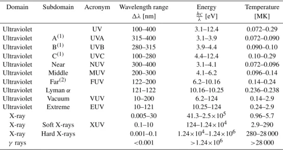
servational data. Before we detail the impact of the solar irradiance on geospace, it is important to specify what we mean by Extreme UltraViolet (EUV) and Soft X-ray (XUV). Different acronyms are used in the literature for describing electromagnetic radiations. A physicist and a physician may well speak of the same radiation without understanding each other; this is why recent studies have been carried out with the aim of standardizing the denominations (it is of course totally out of the question to normalize the solar flux itself). An ISO norm has recently been proposed and is now offi-cially listed as Final Draft International Standard (Tobiska and Nusinov, 2006). The denominations for the different parts of the spectrum are tabulated in Table 1. The wave-lengths we shall focus on range from 0.1 nm to 10 nm (XUV) and from 10 nm to 121 nm (EUV). We will also briefly con-sider the UV range, including the strong Lyman-α line at 121.5 nm.
Our rationale is the impact of these wavelengths on the up-per atmosphere. The solar irradiance in the XUV-EUV range is mostly absorbed by molecular oxygen, atomic oxygen, and molecular nitrogen. The main processes at work are ionisa-tion, excitaionisa-tion, and dissociation. Photoionisation is mostly efficient above 150 km, and filters the light down to about 80 km. The main species involved are O2, N2 and O.
Be-tween 70 and 280 nm, molecular photodissociation becomes an important or predominant process; it filters the light down to low altitudes, typically 20 km. Note that the near ultravio-let (300 to 400 nm) is mostly absorbed by the dissociation of ozone, whose efficiency peaks around 40 km, i.e. far below the altitudes of concern in this review paper.
Table 1.Irradiance ranges with corresponding energies and temperatures in the case of thermodynamic equilibrium. Note that the irradiances are defined by their wavelength and not by their energy range.
(1)Range adopted by the World Health Organisation and the International Commission on Illumination.
(2)Definition adopted in the aeronomy community. Other communities may consider 10 nm instead of 30 nm, and 100 nm instead of 120 nm.
See also the ISO norm project by Tobiska and Nusinov (2006).
Domain Subdomain Acronym Wavelength range Energy Temperature
1λ[nm] hcλ [eV] [MK]
Ultraviolet UV 100–400 3.1–12.4 0.072–0.29
Ultraviolet A(1) UVA 315–400 3.1–3.9 0.072–0.090 Ultraviolet B(1) UVB 280–315 3.9–4.4 0.090–0.10 Ultraviolet C(1) UVC 100–280 4.4–12.4 0.10–0.29 Ultraviolet Near NUV 300–400 3.1–4.1 0.072–0.096 Ultraviolet Middle MUV 200–300 4.1–6.2 0.096–0.14 Ultraviolet Far(2) FUV 122–200 6.2–10.16 0.14–0.24 Ultraviolet Lymanα 121–122 10.16–10.25 0.236–0.238 Ultraviolet Vacuum VUV 10–200 6.2–124 0.14–2.9 Ultraviolet Extreme EUV 10–121 10.25–124 0.24–2.9
X-ray 0.005–30 41.3–2.5×10⁵ 0.96–5.7
X-ray Soft X-rays XUV 0.1–10 124–1.24×10⁴ 2.9–290 X-ray Hard X-rays 0.001–0.1 1.24×10⁴–1.24×10⁶ 280–28 000
γrays <0.001 >1.24×10⁶ >28 000
description of the physics may be found in Lilensten (1999) and in Schunk and Nagy (2004). The impact of the XUV-EUV fluxes on space weather through the atmospheric sys-tem are important. Let us mention the three principal ones. 1.1 Satellite drag: a thermospheric process
One of the prime motivations for nowcasting and forecast-ing the solar XUV-EUV flux is the specification of atmo-spheric densities for spacecraft orbit determination, attitude control, and also for debris mitigation. When an object (spacecraft, or debris) travels through an atmosphere, it ex-periences a drag force opposite to the direction of its motion. As a first approximation, this drag force depends on the ther-mospheric density, the satellite velocity, the satellite cross-sectional area and a drag coefficient. The evaluation of the drag force is conditioned by the knowledge of the thermo-spheric density, which usually comes out of a model. The sources of density variations in the thermosphere are primar-ily the XUV and EUV fluxes, particle precipitation and elec-tric fields. The physical processes involve photo-absorption, particle collisions, Joule heating and frictional heating. For space weather, the main consequence (amongst other phe-nomena) is a dilatation of the thermosphere. During periods of strong solar activity, the density may increase by a fac-tor of 10 at the altitude of the International Space Station (400 km).
The prime goal of satellite operators is to predict the posi-tion of a space object with a accuracy of at least 20 km after 24 h. This prediction requires a permanent monitoring and adjustment of the drag equation through neutral atmosphere
models. Several methods are currently used: the proxy ap-proach, which relies on indices, today still remains important and is difficult to bypass for long-term studies. A technolog-ical approach consists of estimating the thermospheric drag using a reference object, such as a spacecraft with a well-determined cross section (Marcos et al., reported in Nicholas et al., 2000). Physical approaches consist in feeding the mod-els with observations. These observations can, for example, be the UV airglow (Nicholas et al., 2000), the thermospheric temperature (Lathuill`ere et al., 2002), or ionospheric param-eters, such as the Total Electron Content (TEC) (Lilensten and Blelly, 2002).
1.2 Telecommunication and positioning: ionospheric pro-cesses
All existing models (physical, profilers, TEC derived from GPS, . . . ) fail in reproducing the real-time ionosphere, espe-cially at high latitude and during solar events (Jakowski et al., 1999; Lunt et al., 1999; Lilensten et al., 2005). As for the thermosphere, there is a strong need for a permanent moni-toring and adjustment of the equations and the strategy con-sists of using proxies or physical approaches (for example, with topside sounders). The ionosphere, however, is some-what more easily accessible from the ground than from the thermosphere, thereby offering additional opportunities for calibrating models.
1.3 Space weather versus classical weather
Classical weather is somehow out of the scope of this re-view, and yet we mention it here since the different layers of the terrestrial atmosphere are intimately coupled. Several phenomena contribute to these changes; see, for example, the reviews by Haigh (2005), Bard and Frank (2006), and Calis-esi et al. (2006). Some of these processes may be related to space weather. The principal ones are:
– Influence of the total solar irradiance. Records show such an influence over different time scales (Haigh and Blackburn, 2006). The influence of the total solar irra-diance on time scales of decades or less is not as clear as for long-term effects. Typical estimates range from 6% to 30%, with a likely value of about 12% (Alley et al., 2007), which is below the value published 5 years ear-lier by the Intergovernmental Panel on Climate Change.
– Influence of the cosmic rays on condensation nuclei and thereby on cloud cover (Svensmark and Friis-Christensen, 1997; Svensmark, 2007). The micro-physics is described in Harrison and Carslaw (2003). The impact on climate remains controversial as subse-quent studies have failed to confirm a relationship (Laut, 2003; Damon and Laut, 2004).
– Indirect influence of the UV variability: above 30 km, the ozone response is well pronounced (Rozanov et al., 2005; Calisesi and Matthes, 2006). This, in turn, in-fluences the dynamic coupling between the stratosphere and troposphere (Haigh and Blackburn, 2006).
– Influence of the solar wind: some mechanisms have been suggested as early as 1994 (Tinsley, 1994). In particular, Joule heating induced by the solar wind and interplanetary magnetic field may influence the circula-tion and ozone concentracircula-tion in the middle atmosphere (Zubov et al., 2005).
– Impact of greenhouse gases, with, for example, the falling sky theory (Roble and Dickinson, 1989).
– Impact of upper lightning (Sentman et al., 1995) with red sprites, blue jets, elves, etc.
At least the two last ones may be directly related to the ther-mospheric and ionospheric processes.
Let us finally mention the importance of XUV-EUV irradi-ance measurements for modelling radiative transfers in plan-etary atmospheres, for simulating solar cell power and ma-terial degradation. Scientific applications of ultraviolet mea-surements to bodies other than the Sun have recently been reviewed by Brosch et al. (2005).
2 Origin and variations of the XUV-EUV fluxes
The Sun varies on all scales and the variability is strongly de-pendent on the wavelength. For some reviews, see the works by Lean (1987, 1991), Tobiska (1993), Pap et al. (1994) and Woods et al. (2005). Let us briefly examine the various solar origins of this XUV-EUV flux. The UV emission is gener-ated at relatively low temperatures, i.e. in the chromosphere and in the transition region. At the lowest considered temper-atures, there is no local thermodynamic equilibrium in the so-lar atmosphere. The source function can no longer be consid-ered to be a Plank function, and must be evaluated instead by considering each individual atomic process that is involved in the generation of the spectrum. In other words, Table 1 cannot be used to infer the temperature of the formation of a line from its wavelength.
particular at Meudon and at Big Bear observatory (Johannes-son et al., 1995).
Two other Fraunhofer lines in the near UV are impor-tant. Both are due to singly ionized magnesium, at wave-lengths of 280.2 nm (Mg II h line) and 279.5 nm (Mg II k line). The electron transitions involved are similar to those for the Ca II H and K lines, and they are also collisionally controlled. These lines are widely used today as a solar ac-tivity index (Heath and Schlesinger, 1986). The core of the Mg II line is imprinted by the variability of the UV as it orig-inates in the upper chromosphere, as compared to the wings, which are generated in the photosphere and are therefore in-sensitive to solar UV variations. The MgII index is calculated by taking the ratio of the irradiance at the core of the Mg II absorption feature at 280 nm to the average irradiance in the wings of the Mg II feature at approximately 276 and 283 nm. Because of that, the MgII index is a dimensionless quantity which is unaffected by most undesirable effects, such tempo-ral and specttempo-ral changes in the instrument response (Viereck et al., 2001). This index is today derived from various in-struments that differ in resolution, wavelength selection, and derivation method and yet are in excellent agreement (Cebula and Deland, 1998; de Toma et al., 1997; White et al., 1998). Finally, the He II line at 30.4 nm is currently observed by the SEM (Judge et al., 1998) and EIT (Delaboudiniere et al., 1995) instruments on board SOHO, albeit with a resolution of a few nm. This spectral band is dominated by chromo-spheric emissions emitted around 50 000 K. All these quan-tities are strongly correlated both with each other, and with other proxies for solar activity, such as the f10.7decimetric
in-dex, thereby expressing the strong connections between dif-ferent solar atmospheric layers (Floyd et al., 2005).
2.2 UV to XUV emission processes: line emission, free-free and free-free-bound processes
UV and EUV emission processes do not involve neutral atoms or singly charged ions, but multiple charged ions. The collision with an electron generates additional ion-izations if the energy of the incident electron exceeds a threshold (typically 12 eV). We then have an ionization (X+m+e−→X+m+1+2e−), in which the ion is left in an excited state, and goes to a state of lower energy by emit-ting a photon. We can also have radiative recombination (X+m+e−→X+m−1) with the emission of a photon. The
impact with an electron may also leave the ion in an ex-cited state such that it auto-ionizes after a short period of time (X+m∗
→X+m+1+e−
). This excitation can be an elec-tronic recombination (X+m+e−
→X+m−1∗
), where a free electron is captured by the atom. After auto-ionization, the ion is mostly left in a ground state. Some of these processes can also occur with proton collisions or with photoabsorp-tion. These processes, however, have a minor influence. Fi-nally, charge transfer with the abundant hydrogen may leave
the ion in an excited state, from which a photon is emitted (X+m+H→X+m−1∗+H+).
Radiative recombination involves the transfer of a free electron to a captured electron (free-bound process). In the free-free case (or “Bremsstrahlung”), an electron is acceler-ated or deceleracceler-ated through the interaction with a Coulom-bian potential of an ion. These two last processes are re-sponsible for the continuum, in which all frequencies are ex-cited, creating a continuous baseline in the solar spectrum. The other origin of the continuum is the recombination of electrons with bare carbon and oxygen nuclei. The physics involved depends on many parameters, such as the relative abundance of each element, the ionisation ratio, and excita-tion ratio (Arnaud and Rothenflug, 1985; Arnaud and Ray-mond, 1992).
On top of the continuum, several lines are worth examin-ing. In the X-ray range, two resonance lines in the Fe XIV spectrum at 5.90 and 5.96 nm are emitted from the 3p ground state to the 4d state. Above active regions, the temperature of the lower corona can increase to about 4×10⁶K. This re-sults in the additional ionization of iron, especially Fe XV and Fe XVII, whose bright emissions motivated the choice of the 28.4 nm band for one of the filters of EIT on board SOHO (Delaboudiniere et al., 1995).
In the XUV range, resonance lines of helium-like ions of light elements arise, such as carbon (C V) at 4.03 nm, oxygen (O VII) at 2.16 nm and neon (Ne IX) at 1.345 nm. Similarly, there are lines of hydrogen-like ions, equivalent to the Lyman lines of hydrogen itself at UV wavelengths: the Lyαlines of hydrogen-like carbon (C VI) at 3.37 nm and oxygen (O VIII) at 1.90 nm.
In the EUV range, several intense lines are due to lithium-like ions. Lithium has three electrons, with the outer in the n=2 orbit. Excitation may take it from a 2-s sub-orbit to a 2p, and de-excitation back to 2 s results in two closely spaced lines forming a doublet. The lithium-like carbon (C IV) doublet at 155 nm is emitted at transition region tempera-tures. The lithium-like oxygen (O VI) doublet is at 103.2 nm and 103.8 nm, and originates in the coronal region. The lithium-like magnesium (Mg X) is at 61.0 nm and 62.5 nm, and the silicon (Si XII) is at 49.9 nm and 52.1 nm. Fe IX/X at 17.1 nm, which is also observed by EIT, is due to a 3p–3d transition.
2.3 The XUV-EUV-UV spectral variability
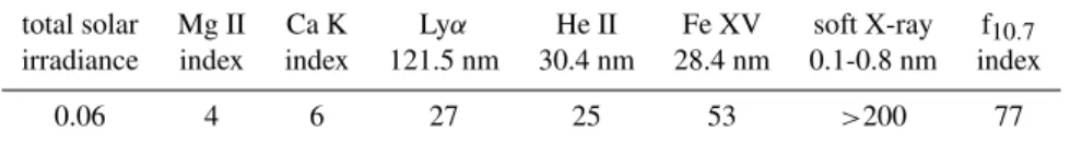
Table 2.Long-term variability (in %) of some spectral lines and EUV/UV indices. The values represent the amplitude of the 11-year cycle normalised to the time average. The total solar irradiance is from SOHO/VIRGO, spectral lines are from TIMED/SEE, and the soft X-ray measurements from GOES/SEM.
total solar Mg II Ca K Lyα He II Fe XV soft X-ray f10.7 irradiance index index 121.5 nm 30.4 nm 28.4 nm 0.1-0.8 nm index
0.06 4 6 27 25 53 >200 77
the XUV-EUV variability, see Lean (1987) and Woods and Eparvier (2006).
The XUV-EUV variability has two components. The short-term and most variable component is associated with sporadic explosive events, such as bright points, flares, and eruptions. The EUV flux is enhanced by these eruptive events because of the temperature increase and electron ac-celeration. Free-free processes are enhanced, and the emis-sion may increase by orders of magnitude (Phillips, 1995), especially in the XUV range (Woods et al., 2005). The sec-ond and slow variability component evolves on times scales of days to years and depends on full disc activity.
3 Are existing XUV-EUV models suitable for space weather?
There are several categories of aeronomical models. The first one consists of models that were first developed in the eighties and that rely heavily on data from Atmospheric Ex-plorer mission (Hinteregger et al., 1973). Many models today still use the binning of the spectrum that was first proposed by Torr and Torr (1979). The success of this approach has to do with its simplicity and the existence of a set of ab-sorption cross sections for each wavelength bin. There are two reference fluxes: one for active and one for quiet condi-tions. Other levels of activity are modelled by interpolating the decimetric index f10.7. In the mean time, the
experimen-tal data used to determine the flux has gradually improved (Hinteregger, 1981; Hinteregger and Katsura, 1981; Torr and Torr, 1985).
Tobiska (1991) and Tobiska and Eparvier (1998) devel-oped a different model, called EUV, using a more extended database. In comparison to the previous ones, this model re-trieves the solar flux from the decimetric index and its aver-age. The latest versions use new input parameters computed from a previous version of the code (Tobiska et al., 2000). EUVAC (Richards et al., 1994) is based on a reference flux that differs from the one used by Torr and Hinteregger, and relies on specific interpolation formula. EUVAC also adds physical constraints on the coronal flux. Its latest version, named HEUVAC (Richards et al., 2006), extends the EUV model below 5 nm and includes data from the SEE instru-ment on board TIMED (Woods et al., 2005).
All these models are valuable tools for aeronomic stud-ies. None of them, however, can properly track solar activity. There are several reasons for this. The first one is the lack of data as the observations span at best 2 solar cycles. Secondly, because the observations are discontinuous in time, not all geophysical conditions are properly covered. Third, due to historical reasons, the wavelength resolution is rather coarse, with generally 39 bins. Finally, all these models rely on one or a few indices that only partly describe the multiple facets of solar activity. As shown by Dudok de Wit et al. (2007), none of the indices is representative of the variability of the EUV spectrum at all wavelengths. Therefore, accurate fore-casting cannot fully rely on any of these models, regardless of their (numerous) qualities.
The second category of models uses additional inputs to reach better accuracy. The Flare Irradiance Spectral Model (FISM) is based on data from TIMED. FISM is an empir-ical model that estimates the solar irradiance from 0.1 to 190 nm with a 1-nm resolution, and with a time cadence of 60 s (Chamberlin et al., 2006). FISM can therefore model both eruptive events (for which very few accurate measure-ments exist) and long-term effects. Its inputs are traditional proxies (Mg II, f10.7, and Lyα) and the irradiance in several
bands (0–4 nm, 30.5 nm, 36.5 nm) to model the daily com-ponent. FISM also makes use of soft X-ray measurements from GOES (0.1–0.8 nm) to model flares. This model is the first one that can be used for near real-time space weather operations.
cannot properly reproduce the observed irradiances below 160 nm. Such discrepancies are inevitable as the underly-ing conditions are not all fulfilled: not all lines are optically thin, assumptions need to be made on the pressure, temper-ature and electron density profiles, relative abundances must be known, etc. (Kretzschmar et al., 2004). In spite of these limitations, models such as NRLEUV2 are valuable tools for research. Their relevance for space weather operations is as yet more questionable.
4 Trying to retrieve the XUV-EUV fluxes from their ef-fects is illusory
Since the impact of the XUV-EUV solar flux on the iono-sphere is well understood, it is tempting to infer this flux from its effects. The reconstruction of the total solar irra-diance from atmospheric effects has recently been reviewed by Krivova and Solanki (2005). Our interest is in the connec-tion between the solar EUV-XUV flux and the thermosphere-ionosphere system. The variation of ionospheric parame-ters, such as the electron density profile as measured at one location by incoherent scatter radar, has been discussed by Mikhailov and Schlegel (2000) and Zhang et al. (2002). To extend this approach to a larger area, one may consider the critical frequency in the E region (Nusinov, 2006). Ther-mospheric parameters have also been used. Strickland et al. (2004) made an attempt to derive the solar flux from terres-trial dayglow observations in the far ultraviolet. The bright-est oxygen emissions (red and green lines) have been used by Singh and Tyagi (2002). In each case, the impact of the flux must be isolated and modelled by a kinetic and/or fluid ionospheric and/or thermospheric code.
The importance of these approaches should not be under-estimated as they offer an excellent way for validating or re-futing solar flux models. Most of them, however, are not suitable for space weather purposes. One of the obstacles is the multiplicity of intricate phenomena. A flare, for ex-ample, enhances the XUV-EUV flux, but also increases the electric field, which alters the dynamics of the ionosphere, heating the lower layers and thereby modifying the ion com-position and the exospheric temperature, which, in turn, is an input parameter for some thermospheric codes. These pro-cesses are so complex and so much entangled that their solu-tions are not necessarily unique (Lilensten and Blelly, 2002). Moreover, all codes depend on internal physical and chemi-cal parameters (e.g. absorption cross sections, collision cross sections) that are known with limited accuracy.
The thermospheric impact of the variability of the solar flux is equally difficult to use. Culot et al. (2005) have shown that the green line is not sensitive enough to geomagnetic ac-tivity in order to be used as a thermospheric tracer for space weather. Let us do a simple calculation for the case of the ionosphere: the primary electron production (due to pho-toionization) is roughly proportional to the total XUV-EUV
solar flux, as it is described by the Beer-Lambert law (Lilen-sten et al., 1989). The additional production from electron collisions (secondary production) is also sensitive to solar activity. In the E and lower F regions, this additional pro-duction may double (quiet conditions) or triple (active condi-tions) the primary production. At higher altitude, the effect is about constant (30% of the primary production). In the E and lower F regions, the electron density is roughly proportional to the square root of the production (Schlegel, 1988). A vari-ation of the solar irradiance by, say, 33% then results in a variation of the electron production rate by less than 100% (3 times the irradiance variation) and a variation of the electron density of about 10%. This value approximately equals the error bar for the most accurate measurements made by inco-herent scatter radars; it certainly exceeds the precision on the TEC, as derived from global positioning measurements. To conclude, even accurate ionospheric measurements presently remain too coarse to evaluate the contribution of various parts of the solar EUV-XUV spectrum. Establishing a correspon-dence between the two is important for research, but trying to retrieve the XUV-EUV fluxes from their impact is illusory.
5 Measuring the whole spectrum is difficult and expen-sive
Making continuous and real-time measurements of the XUV-EUV irradiance has always been a challenge. The instru-ments are costly and sensitive to contamination, their life-time is limited by degradation, and frequent recalibration is required. In a comprehensive review, Schmidtke et al. (2002) show that the spectral coverage of the solar spectrum in the last solar cycles has been far from complete. This has re-sulted in a long hiatus known as the “EUV hole” (Donnelly, 1988; Woods et al., 2005) that has lasted until 2002. A list of present and future missions can be found in Hochedez et al. (2006). Even on board SOHO, the spectrum is not fully measured, although several instruments are devoted to its observation. SUMER (Wilhelm et al., 1995) is a normal incidence spectrometer with two alternate detectors working in UV wavelength, from 50 nm to 161 nm. The spatial reso-lution along the slit has an average value of 1 arcsec and the spectral resolution is about 0.0044 nm. The measurements made by SUMER have been heavily used in the aforemen-tioned works by Warren et al. (1998) and Kretzschmar et al. (2004).
measure the absolute solar EUV flux in the Al bandpass re-gion (17–70 nm) and around the He II line at 30.4 nm (Ogawa et al., 1998).
An outstanding instrument that continuously measures the XUV-EUV spectrum since February 2002 is the Solar EUV Experiment (SEE) on board the TIMED spacecraft (Woods et al., 2005). SEE actually consists of 2 parts, an EUV Grat-ing Spectrograph (EGS) that measures the spectrum from 25 to 195 nm with 0.4 nm spectral resolution and a XUV Pho-tometer System (XPS) that measures from 0.1 to 35 nm with a spectral bandpass of 5 to 10 nm. In the frame of this review, SEE is certainly a unique instrument, and is heavily used (e.g. Dudok de Wit et al., 2005; Kretzschmar et al., 2006; Warren, 2006). Unfortunately, XPS is now partly ineffective. Two other relevant instruments are the Large Yield RA-diometer (LYRA) and the EUV Variability Experiment (EVE). LYRA (Hochedez et al., 2006) is a VUV radiometer on board PROBA2 (to be launched in 2008) and will mea-sure the spectrum in 4 different bands and with a cadence up to 30 Hz: Lyα(115–125 nm), Herzberg continuum (200– 220 nm), Al channel (17–70 nm) and Zr channel (1–20 nm). The EVE instrumental suite (Woods et al., 2006) on board the Solar Dynamics Observatory (SDO) is a heritage from SEE, with higher spectral resolution, higher temporal ca-dence, and better accuracy. The launch of SDO is planned in 2008, with a nominal lifetime of 5 years. EVE consists of several instruments: the Multiple EUV Grating Spectro-graph (MEGS) is a set of 2 spectroSpectro-graphs that measure the 5–105 nm spectral irradiance with 0.1 nm spectral resolution and with 10-s cadence. Part of the MEGS-A CCD is directly illuminated to measure the individual X-ray photons in the 0–7 nm range with 1 nm or better spectral resolution. The EUV Spectrophotometer (ESP) is a spectrograph that mea-sures the solar irradiance in the 0.1–7 nm, 17–34 nm, and 58– 63 nm bands to provide solar X-ray measurement shortward of 5 nm.
The SEE spectrograph on board TIMED is currently suf-fering from growing degradation and even though EVE will soon take over, long-term measurements of the full XUV-EUV-UV spectrum with sufficient spectral and temporal res-olution are not guaranteed.
6 It is therefore tempting to deduce the whole spectrum from the measurement of a reduced set of lines
One of the most conspicuous properties of the solar XUV-EUV spectrum is remarkably similar time evolutions of most spectral lines, when properly normalised (e.g. Floyd et al., 2005). This raises the question as to whether one could infer the spectral variability from a small ensemble of lines only. One could, for example, assume that the total solar spectrum is a linear superposition of reference spectra that originate from different regions, such as coronal holes, active regions or a quiet Sun. Knowledge of the relative area (or filling
fac-tor) of each of these regions (3 in this example) would then be enough to retrieve the total solar spectrum. Conversely, by measuring the total spectrum and its variability, one could, in principle, estimate the filling factors, which are an important input for EUV irradiance models (Warren, 2006) and also for total irradiance models (Wenzler et al., 2006).
This idea of defining reference spectra has been used in the aforementioned studies by Kretzschmar et al. (2004) and Warren (2006). There are some limitations in this. The first one is the lack of crisp definition of what a quiet Sun actually is. Reference spectra formally cannot be constant and must vary in time because of the heterogeneous and dy-namic nature of the solar upper atmosphere. Another prob-lem is the lack of observational data, which hinders the defi-nition of a reference flux for the corona or for active regions. Lastly, the number of reference spectra is not known a pri-ori. These problems can be alleviated by following a more statistical approach, in which the reference spectra are de-termined by blind source separation techniques. Such tech-niques have recently been developed for spectral unmixing problems (Moussaoui et al., 2006). Their main assumption is that the total spectrum is a linear combination of the un-known reference spectra. Their objective is to jointly es-timate these unknown spectra and their contribution to the total spectrum, using statistical hypotheses such as indepen-dence and imposing a structural positivity constraint. Prelim-inary results have shown that three reference spectra suffice for reconstructing the spectral variability (S. Moussaoui and P.-O. Amblard, personal communication, 2007).
A conceptually different approach consists in retrieving the whole spectrum from the observation of a selected set of lines, spectral bands or proxies. The aforementioned FISM model (Chamberlin et al., 2006), is based on this. Such a reconstruction can be done using either physical considera-tions, or a statistical approach. Knowledge of the emission intensity of a given ion gives a lot of information about its ex-citation state. Using quantum mechanics, one can, in princi-ple, recover the other states and therefore the other emission intensities. This property is actually used in the reconstruc-tion of the DEM. Using this approach with the CHIANTI atomic database for emission lines, Kretzschmar et al. (2006) showed that the EUV spectrum can be reconstructed with a relative error smaller than 10%. More important is their re-sult showing that no more than 6 to 10 lines are needed to reach this level of accuracy. By combining this approach with the previous one, one could infer reference spectra from the DEM for various solar regions, and from this reconstruct the total spectrum. An important property here is equality be-tween the DEM of the sum of the contributions and the sum of the DEM from each contribution (Pottasch, 1963). This idea underlies the work by Warren et al. (1998).
the Singular Value Decomposition (SVD) method (Golub and Van Loan, 2000). The SVD is commonly used in mul-tivariate statistics to replace an ensemble of correlated vari-ables by a smaller set of new varivari-ables, whose linear com-bination captures the main features of the original data. Us-ing the SVD, a basic set of lines was extracted, from which the salient features of the spectral variability could be recon-structed. A first result is that 5 to 8 of these lines are sufficient for reconstructing the spectrum between 25 and 195 nm with a relative error below 7%, in excellent agreement with the study by Kretzschmar et al. (2006). The second important outcome is a strategy for determining the most appropriate lines. For a given number of lines, several possible combi-nations give almost equally good results. In determining the best combination, it is important to note that the choice of an observational set should be application-driven. Lilensten et al. (2007), for example, determined the sets that are suited for thermospheric studies by determining the impact of indi-vidual lines on the ionosphere. The best set consists of H I at 102.572 nm, C III at 97.702 nm, O V at 62.973 nm, He I at 58.433 nm, Fe XV at 28.415 nm, and He II at 30.378 nm. It is noticeable that the HeII line is blended by SiXI line but the two lines behave differently as the first one is optically thick and the second one optically thin. The characterization of the dynamics which is the aim of this set is therefore not affected by this blending.
A third alternative is to use an artificial neural network as a flexible nonlinear model for fitting the XUV-EUV irradiance at given wavelengths, using a set of inputs that could include spectral lines, soft X-ray channels, etc. Such black-box mod-els are now increasingly used for space weather applications, such as the forecast of the total electron content (Tulunay et al., 2006).
All these studies provide a strong incentive for an instru-ment that would allow the full XUV-EUV spectrum to be recovered in real time from a few channels (spectral bands). Instead of using a full-fledged spectrograph, the flux would be measured by diodes, for which more robust technologies are being developed (Benmoussa et al., 2006). The methods we have described are excellent for nowcasting. Forecast-ing is a much more challengForecast-ing task, which not only requires continuous XUV-EUV measurements, but also imaging of the Sun in several wavelengths and a better understanding of precursors. The slowly varying contribution of the quiet Sun is relatively easy to model, but forecasting the impulsive contribution of flares is still beyond reach.
7 Conclusion
The XUV-EUV solar flux is a key parameter for space weather. This quantity is still poorly known and spectrally resolved measurements are scarce. There are several ap-proaches for reconstructing the intensities at all wavelengths, using either proxies or by modelling the impact on the
iono-sphere. None of them are really suited for space weather applications, even if they all have their advantages, espe-cially for solar-terrestrial research. Determining the XUV-EUV spectrum in real-time (or in near real-time), and for the long term is a real challenge. This objective is now within reach. Forecasting is still outside our current capabilities.
The next decades should see new concepts emerge. Spectro-imaging, even with coarse spatial resolution, would be of great interest for solar physics. As far as space weather is concerned, the reconstruction of the XUV-EUV flux from a linear combination of a few carefully chosen diode mea-surement would be of considerable interest. Because such an instrument would be lighter, cheaper and more robust than present spectrographs, it could piggyback on other space-craft. The space weather community will soon have a chance to test this concept thanks to the simultaneous operation of LYRA on board PROBA2 and the EVE suite on board SDO. Acknowledgements. The authors of this paper thank the COST 724 community for financial and scientific support.
Topical Editor W. Kofman thanks S. Koutchmy and W. Schmutz for their help in evaluating this paper. He also thanks F. Lefeuvre for his help in evaluating this paper.
References
Alley, R. B., Berntsen, T., Bindoff, N. L., et al.: Climate Change 2007: The Physical Science Basis. Contribution of Working Group I to the Fourth Assessment Report of the Intergovern-mental Panel on Climate Change, Cambridge University Press, Cambridge, 2007.
Arnaud, M. and Rothenflug, R.: An updated evaluation of recom-bination and ionization rates, Astron. Astrophys., 60, 425–457, 1985.
Arnaud, M. and Raymond, J. C.: Iron ionization and recombination rates and ionization equilibrium, Astrophys. J., 398, 394–406, 1992.
Bard, E. and Frank, M.: Climate change and solar variability: What’s new under the sun?, Earth Planet. Sci. Lett., 248, 1–2, doi:10.1016/j.epsl.2006.06.016, 2006.
Benmoussa, A., Theissen, A., Scholze, F., et al.: Performance of diamond detectors for VUV applications, Nuclear Instru-ments and Methods in Physics Research A, 568, 398–405, doi:10.1016/j.nima.2006.06.007, 2006.
Brosch, N., Davies, J., Festou, M. C., and G´erard, J.-C.: A View to the future: Ultraviolet studies of the solar system, Astrophys. Space Science, 303, 103–122, doi:10.1007/s10509-005-9027-2, 2005.
Calisesi, Y. and Matthes, K.: The middle atmospheric ozone re-sponse to the 11-year solar cycle, Space Sci. Rev., 125, 273–286, doi:10.1007/s11214-006-9063-4, 2006.
Calisesi, Y., Bonnet, R.-M., Gray, L., Langen, J., and Lockwood, M. (Eds.): Solar variability and planetary climates, Springer Verlag, Berlin, 2006.
Chamberlin, P. C., Woods, T. N., and Eparvier, F. G.: New flare model using recent measurements of the solar ultraviolet irradiance, in: 36th COSPAR Scientific Assembly, vol. 36 of COSPAR, Plenary Meeting, pp. 395–406, 2006.
Chapman, S.: The absorption and dissociative or ionizing effect of monochromatic radiation in an atmosphere on a rotating earth , Proc. Phys. Soc., 43, 26–45, 1931a.
Chapman, S.: The absorption and dissociative or ionizing effect of monochromatic radiation in an atmosphere on a rotating earth part II. Grazing incidence , Proc. Phys. Soc., 43, 483–501, 1931b. Chapman, S.: Note on the Grazing-Incidence Integral Ch(x, χ) for Monochromatic Absorption in an Exponential Atmosphere, Proc. Phys. Soc. B, 66, 710–712, 1953.
Cook, J. W., Newmark, J. S., and Moses, J. D.: Coronal thermal structure from a differential emission measure map of the Sun, in: ESA SP-446: 8th SOHO Workshop: Plasma Dynamics and Diagnostics in the Solar Transition Region and Corona, edited by: Vial, J.-C. and Kaldeich-Sch¨u, B., 8, 241–244, 1999. Culot, F., Lathuill`ere, C., and Lilensten, J.: Influence of
geomag-netic activity on the O I 630.0 and 557.7 nm dayglow, J. Geophys. Res., 110, 1304, doi:10.1029/2004JA010667, 2005.
Damon, P. E. and Laut, P.: Pattern of Strange Errors Plagues So-lar Activity and Terrestrial Climate Data, EOS Transactions, 85, 370–374, doi:10.1029/2004EO390005, 2004.
de Toma, G., White, O. R., Knapp, B. G., Rottman, G. J., and Woods, T. N.: Mg II core-to-wing index: Comparison of SBUV2 and SOLSTICE time series, J. Geophys. Res., 102, 2597–2610, doi:10.1029/96JA03342, 1997.
Delaboudiniere, J.-P., Artzner, G. E., Brunaud, J., et al.: EIT: Extreme-Ultraviolet Imaging Telescope for the SOHO Mission, Solar Phys., 162, 291–312, 1995.
Donnelly, R.: Gaps between solar UV and EUV radiometry and at-mospheric sciences, in: Solar Radiative Output Variation, edited by: Foukal, P., pp. 139–145, 1988.
Dudok de Wit, T., Lilensten, J., Aboudarham, J., Amblard, P.-O., and Kretzschmar, M.: Retrieving the solar EUV spectrum from a reduced set of spectral lines, Ann. Geophys., 23, 3055–3069, 2005,
http://www.ann-geophys.net/23/3055/2005/.
Dudok de Wit, T., Kretzschmar, M., Aboudarham, J., Amblard, P.-O., Auch`ere, F., and Lilensten, J.: Which solar EUV indices are best for reconstructing the solar EUV irradiance?, Adv. Space Res., in press, 2007.
Floyd, L., Newmark, J., Cook, J., Herring, L., and McMullin, D.: Solar EUV and UV spectral irradiances and solar indices, J. At-mos. Terr. Phys., 67, 3–15, 2005.
Golub, G. H. and Van Loan, C. F.: Matrix Computations, Johns Hopkins Press, Baltimore, 2000.
Haigh, J. D.: The Earth’s climate and its response to solar variabil-ity, in: Saas-Fee Advanced Course 34: The Sun, Solar Analogs and the Climate, edited by: R¨uedi, I., G¨udel, M., and Schmutz, W., pp. 1–107, 2005.
Haigh, J. D. and Blackburn, M.: Solar influences on dynamical cou-pling between the stratosphere and troposphere, Space Sci. Rev., 125, 331–344, doi:10.1007/s11214-006-9067-0, 2006.
Harrison, R. G. and Carslaw, K. S.: Ion-aerosol-cloud pro-cesses in the lower atmosphere, Rev. Geophys., 41, 2–1, doi:10.1029/2002RG000114, 2003.
Heath, D. F. and Schlesinger, B. M.: The Mg 280-nm doublet as
a monitor of changes in solar ultraviolet irradiance, J. Geophys. Res., 91, 8672–8682, 1986.
Hinteregger, H. E.: Representation of Solar EUV Fluxes for Aero-nomical Applications, Adv. Space Res., 1, 39–52, 1981. Hinteregger, H. E. and Katsura, F.: Observational, Reference and
Model Data on Solar EUV, from Measurements on AE-E, Geo-phys. Res. Lett., 8, 1147–1150, 1981.
Hinteregger, H. E., Bedo, D. E., and Manson, J. E.: The EUV spec-trophotometer on Atmosphere Explorer, Radio Sci., 8, 349–354, 1973.
Hochedez, J.-F., Schmutz, W., Stockman, Y., et al.: LYRA, a so-lar UV radiometer on Proba2, Adv. Space Res., 37, 303–312, doi:10.1016/j.asr.2005.10.041, 2006.
Jakowski, N., Schl¨uter, S., and Sardon, E.: Total electron content of the ionosphere during thegeomagnetic storm on 10 January 1997, J. Atmos. Terr. Phys., 61, 299–307, 1999.
Johannesson, A., Marquette, W., and Zirin, H.: Reproduction of the LymanαIrradiance Variability from Analysis of Full-Disk Images in the CaII K-Line, Solar Phys., 161, 201–204, 1995. Judge, D. L., McMullin, D. R., Ogawa, H. S., Hovestadt, D.,
Klecker, B., Hilchenbach, M., Mobius, E., Canfield, L. R., Vest, R. E., Watts, R., Tarrio, C., Kuehne, M., and Wurz, P.: First so-lar EUV irradiances obtained from SOHO by the CELIAS/SEM, Solar Phys., 177, 161–173, 1998.
Kretzschmar, M., Lilensten, J., and Aboudarham, J.: Variability of the EUV quiet Sun emission and reference spectrum using SUMER, Astron. Astrophys., 419, 345–356, doi:10.1051/0004-6361:20040068, 2004.
Kretzschmar, M., Lilensten, J., and Aboudarham, J.: Retrieving the solar EUV spectral irradiance from the observation of 6 lines, Adv. Space Res., 37, 341–346, doi:10.1016/j.asr.2005.02.029, 2006.
Krivova, N. A. and Solanki, S. K.: Modelling of irradiance varia-tions through atmosphere models., Memorie della Societa Astro-nomica Italiana, 76, 834–+, 2005.
Lathuill`ere, C., Gault, W. A., Lamballais, B., Rochon, Y. J., and Solheim, B. H.: Doppler temperatures from O1D airglow in the daytime thermosphere as observed by the Wind Imaging Inter-ferometer (WINDII) on the UARS satellite, Ann. Geophys., 20, 203–212, 2002,
http://www.ann-geophys.net/20/203/2002/.
Lathuill`ere, C., Menvielle, M., Lilensten, J., Amari, T., and Radi-cella, S. M.: From the Sun’s atmosphere to the Earth’s atmo-sphere: an overview of scientific models available for space weather developments, Ann. Geophys., 20, 1081–1104, 2002, http://www.ann-geophys.net/20/1081/2002/.
Laut, P.: Solar activity and terrestrial climate: an analysis of some purported correlations, J. Atmos. Terr. Phys., 65, 801–812, doi:10.1016/S1364-6826(03)00041-5, 2003.
Lean, J. L.: Solar ultraviolet irradiance variations – A review, J. Geophys. Res., 92, 839–868, 1987.
Lean, J. L.: Variations in the Sun’s radiative output, Rev. Geophys., 29, 505–535, 1991.
Leroy, J.-L.: Polarization of light and astronomical observation, vol. 4 of Advances in astronomy and astrophysics, Gordon & Breach Science, 2000.
Lilensten, J. and Blelly, P.-L.: The TEC and F2 parameters as trac-ers of the ionosphere and thermosphere, J. Atmos. Terr. Phys., 64, 775–793, 2002.
Lilensten, J., Kofman, W., Wisemberg, J., Oran, E. S., and De-vore, C. R.: Ionization efficiency due to primary and secondary photoelectrons – A numerical model, Ann. Geophys., 7, 83–90, 1989,
http://www.ann-geophys.net/7/83/1989/.
Lilensten, J., Delorme, P., Samouillan, S., Engel, E., and Barth´el´emy, M.: Influence of the thermosphere on electromag-netic waves propagation: Application to GPS signal, Radio Sci., 40, 3057–3069, doi:10.1029/2004RS003057, 2005.
Lilensten, J., Dudok de Wit, T., Aboudarham, J., Auch`ere, F., and Kretzschmar, M.: How to choose an observed set of solar lines for aeronomy driven applications, Ann. Geophys., in press, 2007. Lunt, N., Kersley, L., and Bailey, G. J.: The influence of the protonosphere on GPS observations: Model simulations, Radio Sci., 34, 725–732, doi:10.1029/1999RS900002, 1999.
Mikhailov, A. V. and Schlegel, K.: A self-consistent estimate of O++ N
2 – rate coefficient and total EUV solar flux with
λ<1050 ˚Ausing EISCAT observations, Ann. Geophys., 18, 1164–1171, 2000,
http://www.ann-geophys.net/18/1164/2000/.
Moussaoui, S., Brie, D., Mohammad-Djafari, A., and Carteret, C.: Separation of non-negative mixture of non-negative sources us-ing a Bayesian approach and MCMC samplus-ing, IEEE Transac-tions on Signal Processing, 11, 4133–4145, 2006.
Nicholas, A. C., Picone, J. M., Thonnard, S. E., Meier, R. R., Dy-mond, K. F., and Drob, D. P.: A methodology for using optimal MSIS parameters retrieved from SSULI data to compute satel-lite drag on LEO objects, J. Atmos. Terr. Phys., 62, 1317–1326, 2000.
Nusinov, A. A.: Ionosphere as a natural detector for investigations of solar EUV flux variations, Adv. Space Res., 37, 426–432, doi:10.1016/j.asr.2005.12.001, 2006.
Ogawa, H. S., Judge, D. L., McMullin, D. R., Gangopadhyay, P., and Galvin, A. B.: First-year continuous solar EUV irradiance from SOHO by the CELIAS/SEM during 1996 solar minimum, J. Geophys. Res., 103, 1, 1998.
Pap, J. M. and Fr¨ohlich, C.: Total solar irradiance variations, J. Atmos. Terr. Phys., 61, 15–24, 1999.
Pap, J. M., Froehling, H. R., Hudson, H. S., and Solanki, S. K. A., eds.: The Sun as a variable star: solar and stellar irradiance vari-ations, vol. 96, Cambridge University Press, Cambridge, 1994. Phillips, K. J. H.: Guide to the Sun, Cambridge University Press,
Cambridge, 1995.
Pottasch, S. R.: The lower solar corona: interpretation of the ultra-violet spectrum., Astrophys. J., 137, 945–966, 1963.
Richards, P. G., Fennelly, J. A., and Torr, D. G.: EUVAC: A solar EUV flux model for aeronomic calculations, J. Geophys. Res., 99, 8981–8992, 1994.
Richards, P. G., Woods, T. N., and Peterson, W. K.: HEUVAC: A new high resolution solar EUV proxy model, Adv. Space Res., 37, 315–322, doi:10.1016/j.asr.2005.06.031, 2006.
Roble, R. G. and Dickinson, R. E.: How will changes in carbon dioxide and methane modify the mean structure of the meso-sphere and thermomeso-sphere?, Geophys. Res. Lett., 16, 1441–1444, 1989.
Rozanov, E., Schraner, M., Egorova, T., Ohmura, A., Wild, M.,
Schmutz, W., and Peter, T.: Solar signal in atmospheric ozone, temperature and dynamics simulated with CCM SOCOL in tran-sient mode, Memorie della Societa Astronomica Italiana, 76, 876–888, 2005.
Schlegel, K.: Auroral zone E-region conductivities during solar minimum derived from EISCAT data, Ann. Geophys., 6, 129– 137, 1988,
http://www.ann-geophys.net/6/129/1988/.
Schmidtke, G., Tobiska, W. K., and Winningham, D.: TIGER-program for thermospheric-ionospheric geospheric research Long-term measurement of solar EUV/UV fluxes for thermospheric-ionospheric (T/I) modelling and for space weather investigations, Adv. Space Res., 29, 1553–1559, 2002. Schunk, R. W. and Nagy, A. F.: Ionospheres, Cambridge University
Press, Cambridge, 2004.
Sentman, D. D., Wescott, E. M., Osborne, D. L., Hampton, D. L., and Heavner, M. J.: Preliminary results from the Sprites94 air-craft campaign: 1. Red sprites, Geophys. Res. Lett., 22, 1205– 1208, 1995.
Singh, V. and Tyagi, S.: Testing of solar EUV flux models using 5577 ˚A, 6300 ˚A and 7320 ˚A dayglow emissions, Adv. Space Res., 30, 2557–2562, 2002.
Strickland, D. J., Lean, J. L., Meier, R. R., Christensen, A. B., Pax-ton, L. J., Morrison, D., Craven, J. D., Walterscheid, R. L., Judge, D. L., and McMullin, D. R.: Solar EUV irradiance variability de-rived from terrestrial far ultraviolet dayglow observations, Geo-phys. Res. Lett., 31, 3801, doi:10.1029/2003GL018415, 2004. Svensmark, H.: Cosmoclimatology: a new theory emerges, Astron.
Geophys., 48, 18–1, doi:10.1111/j.1468-4004.2007.48118.x, 2007.
Svensmark, H. and Friis-Christensen, E.: Variation of cosmic ray flux and global cloud coverage-a missing link in solar-climate relationships, J. Atmos. Terr. Phys., 59, 1225–1232, 1997. Tinsley, B. A.: Solar wind mechanism suggested for weather
and climate change, EOS Transactions, 75, 369–369, doi:10.1029/94EO01010, 1994.
Tobiska, W. K.: Revised solar extreme ultraviolet flux model, J. Atmos. Terr. Phys., 53, 1005–1018, 1991.
Tobiska, W. and Nusinov, A.: ISO 21348 - Process for determining solar irradiances, in: 36th COSPAR Scientific Assembly, vol. 36 of COSPAR, Plenary Meeting, pp. 2621–2630, 2006.
Tobiska, W. K.: Recent solar extreme ultraviolet irradiance obser-vations and modeling: A review, J. Geophys. Res., 98, 18 879– 18 893, 1993.
Tobiska, W. K. and Eparvier, F. G.: EUV97: Improvements to EUV irradiance modeling in the soft X-rays and FUV, Solar Phys., 177, 147–159, 1998.
Tobiska, W. K., Woods, T., Eparvier, F., Viereck, R., Floyd, L., Bouwer, D., Rottman, G., and White, O. R.: The SOLAR2000 empirical solar irradiance model and forecast tool, J. Atmos. Terr. Phys., 62, 1233–1250, 2000.
Torr, M. R. and Torr, D. J.: Ionization frequencies for major ther-mospheric constituents as a function of solar cycle 21, Geophys. Res. Lett., 6, 771–774, 1979.
Torr, M. R. and Torr, D. J.: Ionization frequencies for solar cycle 21: revised, J. Geophys. Res., 90, 6675–6678, 1985.
Viereck, R., Puga, L., McMullin, D., Judge, D., Weber, M., and To-biska, W. K.: The Mg II index: A proxy for solar EUV, Geophys. Res. Lett., 28, 1343–1346, doi:10.1029/2000GL012551, 2001. Warren, H. P.: NRLEUV 2: A new model of solar
EUV irradiance variability, Adv. Space Res., 37, 359–365, doi:10.1016/j.asr.2005.10.028, 2006.
Warren, H. P., Mariska, J. T., and Lean, J.: A new reference spec-trum for the EUV irradiance of the quiet Sun: 1. Emission measure formulation, J. Geophys. Res., 103, 12 077–12 089, 1998.
Wenzler, T., Solanki, S. K., Krivova, N. A., and Fr¨ohlich, C.: Re-construction of solar irradiance variations in cycles 21–23 based on surface magnetic fields, Astron. Astrophys., 460, 583–595, doi:10.1051/0004-6361:20065752, 2006.
White, O. R., de Toma, G., Rottman, G. J., Woods, T. N., and Knapp, B. G.: Effect of spectral resolution on the Mg II index as a measure of solar variability, Solar Phys., 177, 89–103, 1998. Wilhelm, K., Curdt, W., Marsch, E., Schuhle, U., Lemaire, P., Gabriel, A., Vial, J.-C., Grewing, M., Huber, M. C. E., Jordan, S. D., Poland, A. I., Thomas, R. J., Kuhne, M., Timothy, J. G., Hassler, D. M., and Siegmund, O. H. W.: SUMER – Solar Ul-traviolet Measurements of Emitted Radiation, Solar Phys., 162, 189–231, 1995.
Woods, T. N. and Eparvier, F. G.: Solar ultraviolet variability during the TIMED mission, Adv. Space Res., 37, 219–224, doi:10.1016/j.asr.2004.10.006, 2006.
Woods, T. N., Rottman, G. J., Bailey, S. M., Solomon, S. C., and Worden, J. R.: Solar extreme ultraviolet irradiance measure-ments during solar cycle 22, Solar Phys., 177, 133–146, 1998. Woods, T. N., Eparvier, F. G., Bailey, S. M., Chamberlin, P. C.,
Lean, J., Rottman, G. J., Solomon, S. C., Tobiska, W. K., and Woodraska, D. L.: Solar EUV Experiment (SEE): Mission overview and first results, J. Geophys. Res., 110, 1312–1336, 2005.
Woods, T. N., Eparvier, F. G., Jones, A., et al.: The EUV Variability Experiment (EVE) on the Solar Dynamics Observatory (SDO): Science Plan and Instrument Overview, in: ESA SP-617: SOHO-17. 10 Years of SOHO and Beyond, vol. 17, 2006.
Zhang, S.-R., Oliver, W. L., Holt, J. M., and Fukao, S.: Solar EUV flux, exospheric temperature and thermospheric wind in-ferred from incoherent scatter measurements of the electron den-sity profile at Millstone Hill and Shigaraki, Geophys. Res. Lett., 29, 72–1, 2002.