An Automatic Statistical Method to detect the Breast Border in a Mammogram

An Automatic Statistical Method to detect the Breast

Border in a Mammogram

Yee Hung Choy1*, Wai Tak (Arthur) Hung2, Robert A. Mitchell2, Xian Zhou1

1

The Hong Kong Polytechnic University Department of Applied Mathematics Hung Hom, Kowloon, Hong Kong

E-mail: {mayhchoy, maxzhou}@inet.polyu.edu.hk

2

Key University Research Strength in Health Technologies University of Technology, Sydney

Broadway NSW 2007, Australia

E-mail: arthur_hung@hotmail.com, robmitch@eng.uts.edu.au

*

Corresponding author

Received: February 2, 2007 Accepted: Mart 16, 2007

Published: Mart 27, 2007

Abstract: Segmentation is an image processing technique to divide an image into several

meaningful objects. Edge enhancement and border detection are important components of image segmentation. A mammogram is a soft x-ray of a woman’s breast, which is read by radiologists to detect breast cancer. Recently, digital mammography is also available. In order to do computer aided detection on mammogram, the image has to be either in digital form or digitized. A preprocessing step to a digital/digitized mammogram is to detect the breast border so as to minimize the area to search for breast lesion. An enclosed curve is used to define the breast area. In this paper we propose a modified measure of class separability and used it to select the best segmentation result objectively, which leads to an improved border detection method. This new method is then used to analyze a test set of 35 mammograms. The breast border of these 35 mammograms was also traced manually twice to test for their repeatability using Hung’s method1. The borders obtained from the proposed automatic border detection method are shown to be of better quality than the corresponding ones traced manually.

Keywords: Mammogram, Breast border, Area tracing, Validation, Separability.

Introduction

Digital image processing has extensive medical applications. In such applications image processing normally includes preprocessing, segmentation and summarization such as classification. Segmentation of an image into several medically meaningful objects is achieved by boundary and texture analysis, where a boundary of an image is defined as a narrow region where changes in texture occur. Edge enhancement and border detection are important components of image segmentation.

Utilization of a mask allows an algorithm to focus on the analysis of the actual image and significantly improves and speeds up the classification of benign and malignant cases. The generation of a mask is based on the location of the image boundary. In this study we propose an improved method to generate and choose masks based on a modified measure of separability in a two-stage procedure comprising modeling the background of the mammogram and boundary detection. This method is applied on mammograms to detect the breast border so as to minimize the area to search for breast lesion.

Method

The Chandrasekhar and Attikiouzel breast border detection method[5] is used to generate 24 masks for a mammogram. The best mask from a set of masks is selected based on a new measure of separability, which will be defined and explained in details below. A noise cleaning filter described below is used to clean the black and white noise objects in a mask. The first 35 mammograms from Mammographic Image Analysis Society (MIAS) [6] (mdb001 to mdb035) are used for this study.

A computer program was developed to allow a user to trace the breast border manually so as to create a mask. This program has the facility to change the brightness of an image, which helps to identify the border of the breast visually in our study.

These 35 mammograms are traced twice at two occasions. Their repeatability is tested by the Hung’s method [1], and the average percentage relative error is calculated. The detailed calculations are described below. The breast border detection results are compared to those hand traced. The results are presented through the average percentage relative error proposed by Hung [1].

Measure of separability

Thresholding is a well known technique for image segmentation, which attempts to extract objects from their background. The threshold method of Otsu[7] is a global, point dependent technique, which thresholds the entire image with a single threshold value. It is called point dependent (instead of region dependent) because the thresholding value is determined solely from gray level of each pixel (without considering the local property in the neighborhood of each pixel).

Denote by G=

{

}

{

}

{

}

C1 = +1, +2,K, , where kis an element ofG. The number of pixels at gray level i

is denoted by n_i. Then the total number of pixels, N, is given by

∑

=

= L

i i

n N

0

Hence the probability distribution for the occurrence of gray level i is:

N n

P i

i = where Pi ≥0 and 1

0

=

∑

=

L

i i

P

Further define two functions as:

∑

=

= k

i i

P k

0 ) (

ω and

∑

=

= k

i i

P i k

0 ) (

Then µ_T = µ(L) is the expected (or mean) gray level. The Otsu method is based on discriminant analysis, which maximizes the class separability. The recommended discriminant criterion function (or measure of class separability) by Otsu is:

2 2 T B σ σ

η= ,

where

(

)

(

)

B _{ω ω}

µ ω µ σ − −

= and _i

L

i

T

T i P

2 0 2 ) (

∑

are the between-class variance and the total variance of levels, respectively. Since σT2 is

independent of k, maximization of η with respective to kis equivalent to maximizing σB2.

Let k*be the optimal threshold value such that

) ( max )

( * 2

2 2 1 k k B k k k B σ σ ≤ ≤ = ,

where k₁ and k₂ are the gray levels that have the first non-zero n_i when iis in ascending and descending orders respectively.

In the Otsu method, the pixel values in an image are separated into two groups when a k

value is selected. One group consists of the gray levels ranging from 1 to k while the second group contains the remaining levels from k+1 to L.

A mask of an image has identical dimensions of the original image and only two gray levels, 0 and 255. Instead of using a single gray level to define two groups in the Otsu method, a mask is used to create two groups of pixels from the original image according to their corresponding gray levels in the mask. This means that the first group pixels are of gray level 0 in the mask while the second group has the mask gray level of 255. The measure of class separability is then re-defined as follows for the calculations of the two groups of pixels defined by a mask.

Let G₀and G₁ denote the classes of background and object respectively. In both G₀ and G₁, they have gray levels 0,1,2,K,L, where L is the maximum gray level and L+1 is the total number of possible gray levels. Let n_0i and n_1i be the number of pixels at level i for G₀ and

1

G respectively. Then the total number of pixels is:

(

)

∑

The respective probability distribution for the occurrence of gray level i for G₀ and G₁ are:

N n

P i

i

0

0 = and

N n

P i

i

1

1 = , i=0,1,2,K,L

The zeroth- and first-order cumulative moments of the histogram for G₀ are defined respectively as:

∑

ω and

∑

Similarly,

∑

ω and

∑

= = L i i G iP 0 1 1 µ

are the respective moments for G₁. Then a new measure of class separability, η, is re-defined by replacing σ_B2 and σ_T2 with the following new respective terms as:

1 0

0 0

2

2 ( )

G G

G G T

B _{ω ω}

µ ω µ

σ = − and _i

L

i

T

T i P

2 0 2 ) (

∑

(

)

∑

T i n n

N 0 1 0 1 1 0 µ µ µ and N n n P P

P i i

i i i 1 0 1 0 + = + =

are the new mean gray level of the original matrix (or image) and the new probability distribution for the occurrence of gray level i respectively. Since σ_T2 is independent of how

0

G and G₁ are defined and hence is a constant for a given image, comparing η is the same as comparingσ_B2. Therefore, σ_B2 is used for the calculation of the measure of class separability in this study.

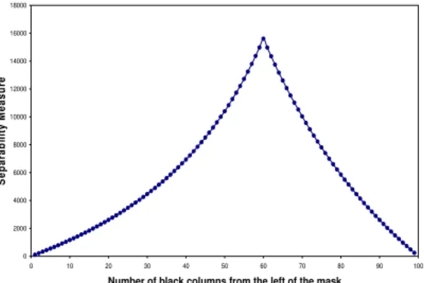
A test image is constructed with a size of 100 times 100 pixels. The first 60 columns starting from the left are black and the rest are white, as shown in Figure 1a. 99 masks are also constructed. Their sizes are identical to the test image but the numbers of black columns varied from 1 to 99. Hence the mask with 60 black columns is identical to the test image. When this mask is applied to the test image, the calculated measure of separability reaches maximum (see the peck in Fig. 1b) because this mask correctly defines the two black and white regions. All the other masks captured a region of mixture of black and white columns of pixels.

Image noise removal algorithm

In order to clean the resulting processed images, small white spots on the background and small black spots within the breast region need to be removed from the binary image. This is achieved with a two pass filtering operation.

0 2000 4000 6000 8000 10000 12000 14000 16000 18000

0 10 20 30 40 50 60 70 80 90 100

Number of black columns from the left of the mask

S e pa ra b il it y M e a s ur e

Fig. 1a A test image of size 100 times 100. The first 60 columns are black and the rest

are white.

Fig. 1b A plot of Separability Measures against a mask of same size of the test image (number of black column(s) from the

left of the mask varies).

The inverse of the resulting image after passing the first filter is then passed through a second “vtkImageIslandRemoval2D” filter, this time with the Area Threshold set to 0.1 times the number of pixels in the image. The output image now has the small black islands removed from the breast region (although the resulting output has its grayscale inverted). Finally, the inverse of this output binary image is taken, resulting in the white breast region on a black background, with no other small white or black islands.

Measure of repeatability

Let X_1j andX_2j be the traced breast areas on a mammogram at two occasions. Also, let I_j

and U_jbe the intersection and union of this pair of traced areas. The average percentage relative error3 of n pairs of mammograms is defined as:

% 100 1 1 × ⎥ ⎥ ⎦ ⎤ ⎢ ⎢ ⎣ ⎡ ′ = ′

∑

X X

m = + and

(

)

2 1 j j j j

j U m U I

d′ = − = −

Here m_jis used to estimate the true breast area in a jth mammogram and d′_j is the estimated error from two tracings on the same mammogram. The e′ is used to evaluate the repeatability of two sets of tracings from a person. One set is then chosen to compare with another set of tracings from the computer detection border method based on the same set of mammograms using the same measure.

Results

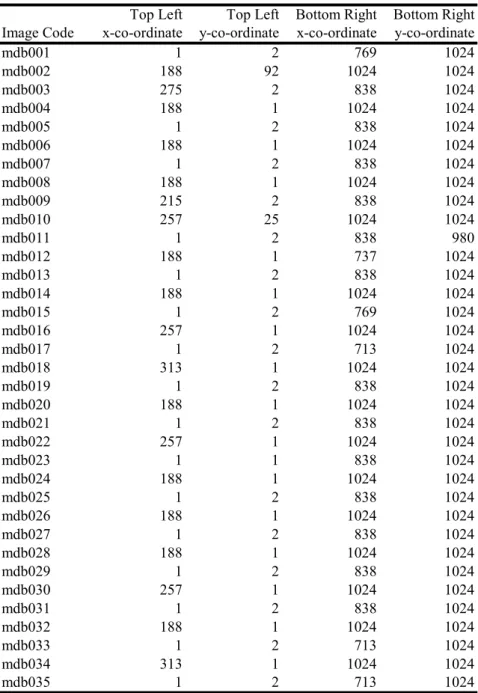
Table 1. Image cropped using the corresponding top left and bottom right x and y coordinates

Top Left Top Left Bottom Right Bottom Right

Image Code x-co-ordinate y-co-ordinate x-co-ordinate y-co-ordinate

mdb001 1 2 769 1024

mdb002 188 92 1024 1024

mdb003 275 2 838 1024

mdb004 188 1 1024 1024

mdb005 1 2 838 1024

mdb006 188 1 1024 1024

mdb007 1 2 838 1024

mdb008 188 1 1024 1024

mdb009 215 2 838 1024

mdb010 257 25 1024 1024

mdb011 1 2 838 980

mdb012 188 1 737 1024

mdb013 1 2 838 1024

mdb014 188 1 1024 1024

mdb015 1 2 769 1024

mdb016 257 1 1024 1024

mdb017 1 2 713 1024

mdb018 313 1 1024 1024

mdb019 1 2 838 1024

mdb020 188 1 1024 1024

mdb021 1 2 838 1024

mdb022 257 1 1024 1024

mdb023 1 1 838 1024

mdb024 188 1 1024 1024

mdb025 1 2 838 1024

mdb026 188 1 1024 1024

mdb027 1 2 838 1024

mdb028 188 1 1024 1024

mdb029 1 2 838 1024

mdb030 257 1 1024 1024

mdb031 1 2 838 1024

mdb032 188 1 1024 1024

mdb033 1 2 713 1024

mdb034 313 1 1024 1024

mdb035 1 2 713 1024

respective mammograms on Figs. 2b and 3b. The Fig. 2f is an example of good result from our method while the result shown in Fig. 3f is fair. In Fig. 3f, the weak edge near the bottom was removed during the noise clean process and hence the corresponding portion of the estimated breast border cut into the breast area.

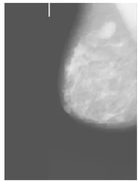
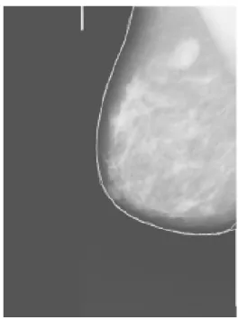
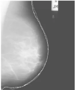
Fig. 2a The original mdb015 image. Fig. 2b The mdb015 image was adjusted with the increased of brightness.

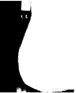
Fig. 2c Mask result obtained from our method

Fig. 2e Lines from first and second tracings (grey and white respectively) were superimposed on the adjusted mdb015

image shown on Fig. 2b

Fig. 2f Line from first tracing and the edge detection line from Fig. 2d (grey and white respectively) were superimposed on the adjusted mdb015 image shown on Fig. 2b

Fig. 3c Mask result obtained from our method

Fig. 3d The mask from Fig. 3c after noise cleaning.

Fig. 3e Lines from first and second tracings (grey and white respectively) were superimposed on the adjusted mdb014

image shown on Fig. 3b

Fig. 3f Line from first tracing and the edge detection line from Fig. 3d (grey and white respectively) were superimposed on the adjusted mdb014 image shown on Fig. 3b

Discussion

We have demonstrated that the modified measure of separability can be used to select a good mask from a set of masks generated from a mammogram in an objective manner. The proposed measure could improve Chandrasekhar et al’s method by removing the more subjective visual inspection step in selecting a mask from a set of 24 masks for a mammogram.

are the corresponding masks after noise cleaning. Fig. 4b is an example to include an undesired label close to the breast area in the final mask. Fig. 5b is another example of including a label in the final mask. In this case the label is quite distant from the breast area.

Fig. 4a A mask obtained by processing mdb005 image

Fig. 4b The corresponding image cleaned by the noise cleaning method

Fig. 5a A mask obtained by processing mdb020 image

Fig. 5b The corresponding image cleaned by the noise cleaning method

mammogram before the breast border detection process. The e′ value will be improved further when this label issue is resolved.

Acknowledgement

This research was partially supported by a Hong Kong Polytechnic University Internal Research Grant.

We thank Miss Candy Lam for her assistance in the computer programming and Mrs. Agnes Chan for tracing the breast border of the selected mammograms from the MIAS. We are also grateful to Professor Hung Nguyen for the use of his PC Tablet for the breast border tracing work.

References

1. Hung W. T. (2006). A New Parameter for Improved Assessment of the Tracing Repeatability of Area Measurements of the Left Ventricle, Bioautomation, 4, 73-79. 2. Singh S., K. Bovis (2002). Medical Image Segmentation in Digital Mammography. In J.

S. Suri, S. K. Setarehdan, S. Singh. (Eds), Advanced Algorithmic Approaches to Medical Image Segmentation, 470-472.

3. Hung W. T., H. T. Nguyen, B. S. Thornton, Y. Zinder (2003). Dynamic Programming Approach to Image Segmentation and Its Application to Pre-processing of Mammograms, Australian Journal of Intelligent Information Processing Systems, 8 (2), 51-56.

4. Wirth M. A. (2006). Performance Evaluation of CADE Algorithms in Mammography, In

J. S. Suri, R. M. Rangayyan (Eds), Recent Advances in Breast Imaging, Mammography, and Computer-Aided Diagnosis of Breast Cancer, 650-653.

5. Chandrasekhar R., Y. Attikiouzel (2000). Segmenting the Breast Border and Nipple on Mammograms, Australian Journal of Intelligent Information Processing Systems, 6 (1), 24-29.

6. The Mini-MIAS database of mammograms: http://peipa.essex.ac.uk/ipa/pix/mias/

7. Otsu N. (1979). A Threshold Selection Method from Gray-Level Histograms, IEEE Transactions on Systems, Man and Cybernetics, SMC-9 (1), 62-66.