Key words: travel behavior, land use, activity participation, socioeconomic variables.
Palavras-Chave: comportamento relacionado a viagens, uso do solo, participação em atividades, variáveis socioeconômicas.
Recommended Citation
* Email: [email protected].
Research Directory
Submitted 11 Jun 2012; received in revised form 29 Oct 2012; accepted 11 Nov 2012
Linking activity participation,
socioeconomic characteristics, land use and travel patterns:
a comparison of industry and commerce sector workers
[Relações entre participação em atividades, características socioeconômicas, uso do solo e padrões de viagens: uma comparação entre trabalhadores nos setores industrial e comercial]
Federal University of Bahia - Brazil, University of São Paulo - Brazil, Technical University of Lisbon (TULisbon) - Portugal
Resumo
O objetivo deste trabalho é analisar o comportamento relacionado a viagens de trabalhadores do setor industrial e comercial, em termos de três grupos de variáveis: participação em atividades, características socioeconômicas e uso do solo. Este trabalho baseia-se na Pesquisa Origem-Destino, realizada na Região Metropolitana de São Paulo (RMSP) em 1997. Foram encontradas relações entre as variáveis consideradas (Árvore de Decisão), e a significância estatística das variáveis independentes (Regressão Linear Múltipla). Foi analisada a influência dos três grupos de variáveis na escolha dos padrões de viagens: (A) Variáveis socioeconômicas (Renda domiciliar, Vale transporte e Posse de automóveis) afetam a sequencia do modo de transporte; (B) Participação em atividades (Estuda e Trabalha) tem um efeito na sequencia dos motivos de viagem; e (C) variáveis de uso do solo (proporção acumulada de empregos por determinado raio a partir dos centroides das zonas de tráfego dos domicílios) influenciam a sequencia de destinos escolhidos, sobretudo para o caso de trabalhadores na indústria. Os diferentes arranjos espaciais das atividades econômicas (comerciais e industriais) na cidade influenciam a viagem dos trabalhadores. Este artigo contribui essencialmente através da proposta de uma variável de uso do solo, proveniente do modelo de oportunidades intervenientes, bem como na apresentação de um método que combina a aplicação conjunta de técnicas de análise multivariada de dados exploratórias e confirmatórias.
Pitombo, C. S., Kawamoto, E. and Sousa, A. J. (2013) Linking activity participation, socioeconomic characteristics, land use and travel patterns: a comparison of industry and commerce sector workers. Journal of Transport Literature, vol. 7, n. 3, pp. 59-86.
Cira Souza Pitombo*, Eiji Kawamoto, Antonio Jorge Gonçalves de Sousa
Abstract
The objective of this work is to analyze the travel behavior of industry and commerce sector workers in terms of three variables groups: activity participation, socioeconomic characteristics and land use. This work is based on the Origin-Destination survey carried out in the São Paulo Metropolitan Area (SPMA) in 1997. Relationships were found between the concerned variables (Decision Tree), and the statistical significance of independent variables was assessed (Multiple Linear Regression). We analyzed the influence of the three variables groups on travel pattern choices: (A) socioeconomic variables (Household Income, Transit Pass Ownership and Car-ownership) affect the travel mode sequence; (B) activity participation (Study, Work) has an effect on the trip purpose sequence; and (C) land use variables (accumulated proportion of jobs by distance buffers starting from the home traffic zone centroid) influence the sequence of destinations chosen, especially in the case of industry sector workers. The different spatial distributions of economic activities (commercial and industrial) in the urban environment influence the travel of workers. This paper contributes essentially proposing the land use variable, through the intervening opportunities model as well as the presentation of a methodology, formed by application of exploratory and confirmatory techniques of multivariate data analysis.
Introduction
The objective of this work is to find relationships between travel patterns (dependent variable)
and the three independent variable groups mentioned before: (A) activity participation; (B)
socioeconomic characteristics; and (C) environmental factors (distribution and degree of
activities, defined as land use variables) considering groups of individuals characterized as
either industry or commerce sector workers.
People generate complex urban travel patterns while engaging in out-of-home activities,
which vary based on individual characteristics, household attributes and environmental
characteristics. One of the objects of the Activity Based Travel Approach is to investigate the
variables that affect travel patterns.
Several authors (Bhat and Singh, 2000; Bowman and Ben-Akiva, 2000; Lu and Pas, 1999;
Strathman and Dueker, 1990) suggested that the journeys of individuals can be influenced by
three main factors: (A) activity participation, (B) socioeconomic characteristics and (C)
environmental factors (urban densities, distances between localities, spatial coverage of the
transportation network, and so on).
The idea that socioeconomic characteristics and activity participation can influence travel
behavior has been studied previously (Arentze et al., 2000; Balasubramaniam and Goulias,
1999; Golob and Mcnally, 1997; Bhat and Koppelman, 1991; Kwan, 2000). The conclusions
in the literature suggest that personal travel can be determined by gender, car ownership
(Strambi et al., 2004; Mcguckin and Murakami, 1999), the role of the person in the family,
household task allocation (Simma and Axhausen, 2001; Srinivasan and Athuru, 2005) and
activity participation (classified as subsistence, leisure, medical, shopping, and so on).
However, socioeconomic characteristics and individual activities are only part of the set of
variables that can allow for the prediction of travel behavior. Not only car ownership, but also
the distribution of activities in the urban environment and accessibility to opportunities affect
modal choice and destination choice. The locations where people live or work exert strong
Environmental factors, such as road infrastructure networking, urban configuration,
localization of activity centers in the cities, density and land use influence travel behavior. In
the present work, environmental factors (land use variables) are defined as the spatial
distribution and degree of activity for each economic sector (industry and commerce).
The assumption that land use policy can influence travel behavior follows from the correlation
between the variables considered. Diverse works confirm that land use (characterized by
urban densities, cities being compact or spread-out, the distribution of economic activities in
urban environments and the presence of Traffic Zones with mixing activities) is strongly
related to travel behavior, especially modal choice (Cervero and Radisch, 1996: Ewing, 1995;
Kitamura et al., 1997). The proposal of the land use variables is one contribution described in
this paper. Besides, we can note in this work, the influence of this variables group on travel
behavior, especially considering workers in industry sectors.
Six steps were performed and are described in the following sections. Section 1 describes the
main characteristics of the study area and the data preprocessing; Section 2 presents the
representation of independent variables: categorical and numeric; Section 3 designates the
representation of the categorical dependent variable; Section 4 - Part 1 (Exploratory Analysis – Classification and Regression Tree (CART) application) – was used to find a priori unknown relations; Section 5 - Part 2 (Confirmatory Analysis – Multiple Linear Regression
(MLR) application) – was applied to verify the statistical significance of the variables and to
corroborate the previously results obtained through CART application; the conclusions finally
1. Study area: São Paulo Metropolitan Area
São Paulo is the largest Brazilian metropolitan area, with a population of over 17 million
distributed over 39 counties, including São Paulo city. Analysis was based on data obtained
during the origin-destination home-interview survey carried out by METRÔ-SP in the São
Paulo Metropolitan Area (SPMA) in 1997.
The region was divided into seven sub-regions and 389 Traffic Zones (TZs). The original
sample contains 98,780 individuals and 28,278 households representing 0.61% of the total
number of the households.
To analyze the behaviors of both industry and commerce sector workers and consider the
hypothesis that the spatial distribution of economic activities in the urban environment affects
the travel of individuals, two different analyses were performed:
(1)Analysis of the spatial distribution of industrial and commercial jobs in the study area
and
(2)analysis of the main changes in the job market of the SPMA, considering the two
economic sectors.
Both analyses are presented in the next two sub-sections. After that, the data treatment and the
resulting sub-samples are described.
1.1 The spatial distribution of industrial and commercial jobs (SPMA)
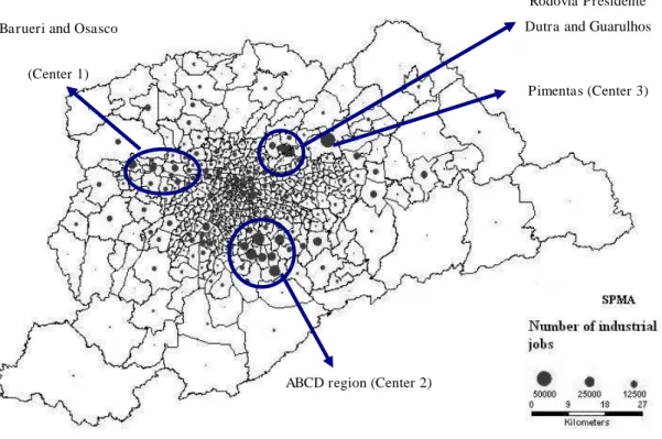
There are concentrations of industry sector jobs (Figure 1) in some specific regions: (1) The
TZs of Pimentas, Rodovia Presidente Dutra and Guarulhos; (2) the ABCD region; and (3) the
counties of Barueri and Osasco. The SPMA basically has three main industrial centers,
Figure 1 - Spatial distribution of industrial jobs. Source: METRÔ-SP
There is a strong concentration of commercial jobs (Figure 2) in the central region. There are
also a great number of commercial jobs in ABCD region and four main centers: (1) The TZs
of Itaquaquecetuba, Suzano and Mogi das Cruzes; (2) Guarulhos and Vila Galvão; (3)
Carapicuíba, Jardim Veloso and Santo Antonio; and (4) Jardim São Luis, Centro Empresarial
and Vila Santa Catarina. Commercial activities are relatively dispersed in the SPMA, with six
main centers of commercial job concentration.
Industrial jobs are concentrated in three main centers located within the study area, while
commercial jobs are scattered over the entire region. Thus, the economic sectors were
analyzed separately to obtain more appropriate results.
The purpose was to reveal the possible influence of land use comparing two specific cases
(industry and commerce sector workers). It was anticipated that land use variables would
exert a greater influence in the case of industry sector workers due the concentration of
industrial jobs in the determined traffic zones.
This analysis can indicate future changes in the travel of individuals, as there is an increase of
jobs in the tertiary sector and a decrease in industrial jobs (sub-section 1.2).
Pimentas (Center 3) Rodovia Presidente
Dutra and Guarulhos
ABCD region (Center 2)
(Center 3) Barueri and Osasco
Figure 2 - Spatial distribution of commercial jobs. Source: METRÔ-SP
1.2 Changes in the job market of the SPMA
Over the past 20 years, the SPMA has undergone significant socioeconomic and demographic
changes, which can be seen in the analysis of the data collected for the Instituto Brasileiro de
Geografia e Estatística (IBGE) and Fundação Estadual de Análise de Dados de São Paulo
(SEADE).
There were considerable changes in the economic activities of the region, mainly in the
1980s. These include:
(1) the reduction of industrial jobs;
(2) the expansion and consolidation of service and commerce activities;
(3) the deterioration of the job market; and
(4) the increase in unemployment taxes and the number of autonomous workers.
As indicated by the IBGE information, the SPMA had an unemployment tax of 3.9% in 1980,
5.8% in 1990 and 8.4% in the first semester of 2002. The participation of autonomous
ABCD region (Center 2) Vila Galvão, Guarulhos (Center 4)
Central region: República,
Brás, Bresser, Parque D.
Pedro.(Center 1)
Carapicuíba Jardim Veloso Santo Antonio (Center 5)
Jardim São Luis Centro Empresarial
Vila Santa Catarina (Center 6)
Itaquaquecetuba
Suzano
Mogi das Cruzes
workers in the job market increased from 19% to 29%, and the participation of the employees
fell from 58% to 48% between 1991 and 2002.
The advance of technology is pointed to as a main reason for the elimination of industrial
jobs. New technologies such as informatics, communications and robotics caused the
disappearance of some occupational categories. Moreover, in the 1980s and 1990s, a
widespread process of industrial decentralization occurred in the state of São Paulo. A great
number of industrial establishments moved from the capital (and its periphery) to other cities,
promoting the increase of urban medium-sized centers and generating new transformations in
the SPMA.
1.3 Data preprocessing
In this stage, incomplete data or those that were not relevant to the objectives were eliminated.
The initial sample was composed of the records for 98,780 individuals, aggregate data of the
home traffic zones of each individual and the Euclidean distances of all the trips. The
following individuals were selected for analysis:
- individuals who made 2, 3 or 4 trips on the day prior to survey;
- individuals who made home-based tour; and
- individuals that work in the industry or commerce sectors.
Finally, considering the differences in the geographic distribution of jobs in the SPMA and
the research hypotheses that the different spatial distributions of economic activities
(commercial and industrial) in the urban environment influence the travel of commerce or
industry sector workers, two sub-samples were identified: (a) industry sector workers and (b)
2. Independent variables representation
The independent variables (categorical or numerical) used in this work belong to the three
main variables groups: (A) socioeconomic characteristics, (B) activity participation and (C)
land use characteristics.
The independent variables selected here are related to travel patterns. The variables of the first
and the second groups were chosen based on the literature and data availability.
(A)Socioeconomic variables: Household income (HI); Car ownership (AUT); Position of
the individual in the family (PF) (1: Head; 2: Spouse; 3: Child; 4: Relative; 5: House
servant; 6: Visitor); Family size (FS); Level of education (LE); Gender; Age; Transit
pass ownership (TP).
(B)Participation in subsistence activities: Work (W) (1: Employee; 2: Autonomous; 3: Unemployed); Study (S) (1: Don’t study; 2: Elementary school; 3: High school and college; 4: Other courses).
The third variable group is proposed based on the principles of the intervening opportunities
model (Schneider, 1959). It will be discussed in detail in the following subsection.
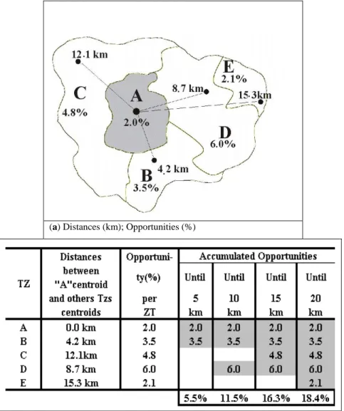
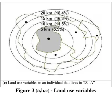
2.1 Land use variables
For elaboration of the land use variables, the intervening model principle was adopted. This
principle assumes that, in the urban area, all trips are as short as possible. Individuals
accomplish long trips only to reach the next acceptable destination, where their purpose is
satisfied. In this work, land use variables are represented in terms of degree of "accumulated
opportunities" for the distance buffer.
In this work, the term "opportunities" refers to the job supply in the economic sector.
Considering the two sub-samples, "opportunities" represents "the proportion (%) of the total
jobs in the industry sector" (for the case of industrial workers) and "the proportion (%) of the
total jobs in the commerce sector" (for the case of commercial workers). These measurements
were collected for various distance buffers starting from the home TZ centroid up to 5, 10 km,
Figure 3 (a, b and c) shows the land use variables. The zone of origin is the shaded area “A”.
At stage (a), the values of the "opportunities" are represented in (%) for each zone together
with straight-line distances from the centroid of "A". In (b), the "accumulated opportunities"
for each of the four distance buffers are shown. Finally, at stage (c), the land use variables from TZ “A” are illustrated.
(a) Distances (km); Opportunities (%)
(c) Land use variables to an individual that lives in TZ “A”
Figure 3 (a,b,c) - Land use variables
The land use variable set defined here represents the distribution and degree of activities in
the urban environment (accumulated opportunities in the industry sector up to 5 km from the
home TZ, accumulated opportunities in the industry sector up to 10 km from the home TZ,
and so on).
3. Coding the categories of the dependent variable
In this study, the trip-linking representation was based on activity sequence, travel mode and
destinations chosen for the individuals in the period of one day. The dependent variable
coding follows the scheme below.
(a) Activity sequence
(b) Travel mode sequence
(c) Sequence of trip destination
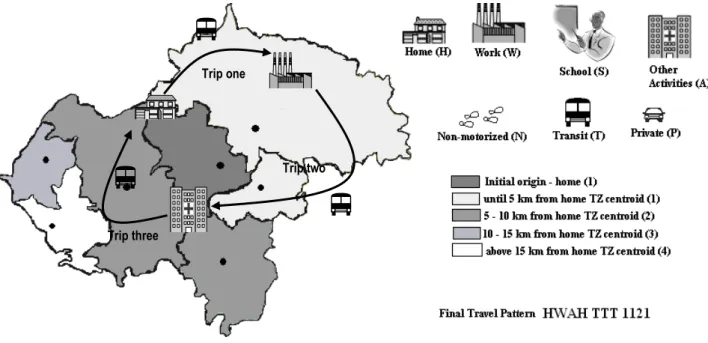
(d) Final Travel Pattern - combination of the previous stages
The travel attributes (activities, travel mode and destinations) were grouped and represented
by letters and numbers, as shown in Table 1. The 128 categories of dependent variables are
attributes. As mentioned before, it was assumed that the individual’s residence was the initial origin and final destination for those who took two, three or four trips.
Table 1 - Travel Patterns Representation
H Home P Private
W Work T Transit
S School N Non-motorized
A Other Activities
1 2 3 4
10-15 kilometers from home TZ centroid above 15 kilometers from home TZ centroid
Step C
Destination (distance to the home Traffic Zone (TZ) centroid) Numbers
until 5 kilometers from home TZ centroid 5-10 kilometers from home TZ centroid Step A
Activity Sequence Letters
Step B
Travel Mode Sequence Letters
In the first step, the travel patterns were represented by a sequence of letters (H, W, S and A)
indicating the sequence of activities performed by the individuals during the day (HSH: home – school – home). In the subsequent stage, the letters (P, T and N) indicate the travel mode sequence used (NN: Non-motorized – Non-motorized).
In the third step, the sequence of destinations was characterized by numbers (1, 2, 3 and 4).
Each one of the numbers represents distance buffers starting from the home zone centroid
(Table 1). The first and last numbers always represent the initial and final destination, the individual’s home (represented by number 1). For example, pattern 141 indicates the accomplishment of two trips: (first trip) starts at home (number 1) and continues to a
destination located more than 15 km away (number 4); (second trip) denotes the return from
destination (4) to the home (number 1).
According to the coding defined in the previous stages, the final travel patterns are
represented by three sets of characters: The first set refers to the activity sequence (e.g.,
HWAH), the second set corresponds to the travel mode sequence (TTT, for example) and the
final set describes the destination sequence (e.g., 1121). The resulting travel pattern HWAH
Figure 4 - Travel patterns (activity, travel mode and destination)
After representing the dependent variable categories, the individuals with less frequent travel
patterns were eliminated in each one of the sub-samples due to the software (S-PLUS 6.1)
limitation of 128 categories of dependent variable. Finally, two sub-samples were obtained:
(a) industrial workers - 4,102 individuals; and (b) commercial employees - 6,043 individuals.
4. Exploratory analysis
The CART (Classification and Regression Tree) algorithm was used in the current research.
This technique allows successive division of a population into binary splits. The resultant
subgroups are homogeneous with respect to the dependent variable, yielding a hierarchical
tree of decision rules useful for prediction or classification (Breiman et al., 1984).
CART is a segmentation modeling technique that satisfies the following properties:
(a) the hierarchy is called tree and each segment is a node;
(b) the root node contains the complete database;
(c) the root node is divided sequentially, generating child nodes;
Trip one
Trip two
Trip three
(d) when no further data subdivision is possible, the final subgroups are considered terminal
nodes or leaves;
(e) for construction of the CART three main elements should be determined: a set of questions
delimiting data division, a criterion for evaluation of the best division and a rule for
termination of further subdivisions (stop-splitting rule); and
(f) each division depends on the value of a unique independent variable. Thus, amongst the set
of independent variables, the one that gives the best split is chosen (greatest segregation of the
data). The procedure continues until no significant splits remain. In this form,
multicollinearity does not cause any problems for the algorithm, therefore, the independent
variables are analyzed separately (Piramuthu, 2008).
Using this technique, two trees were generated from the final sub-samples of industrial and
commercial workers, 128 categories of dependent variable (travel patterns) and numerical and
categorical independent variables (three variable sets mentioned in the work). The trees,
illustrated in Figures 5-6, were generated using at least 50 observations for each leaf node,
using 0.15 for global node deviance (stop-splitting rule) and resulting in 10 leaves for industry
sector workers and 8 leaves for commerce sector workers.
The figures display the CART with the two most frequent travel patterns at each terminal
node (leaves) obtained using SPLUS 6.1. The figures show stages of the construction of the
trees, representing the influence of each variable in travel pattern choices in each sub-sample
and differences of travel behavior between industrial and commercial workers. The
sub-section below describes the influence of each independent variable selected on the travel
behavior of industry and commerce sector workers.
4.1 Independent variable influence: The CART algorithm
The first independent variable selected in the industry sector worker sample was “car
ownership” (AUT). The data were segregated into two branches: (1) branch 1 - AUT=0
(terminal nodes 11; 20; 21; 8 and 9); and (2) branch 2 – AUT > 1 (terminal nodes 7; 27; 53;
In analysis of the commerce sector workers sample, “car ownership” was selected for the
second split: (1) AUT=0 (terminal nodes 21; 20 and 8); and (2) AUT > 1 (terminal nodes 19;
18 and 10).
Figure 5 (a) shows the “car ownership” influence. In both samples, individuals that had cars
at the household used an automobile in travel sequences most frequently. According to the
terminal nodes and the two predominant travel patterns, people that do not have cars at the
household predominantly use transit or non-motorized travel modes (TT, NN, NNNN, NNN).
There is a predominance of car usage in individuals who have at least one car at the household
(PP, PPP).
Figure 5 - CART construction (a) Car Ownership influence
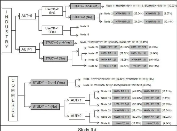
As seen in Figure 5 (b), the participation of individuals in scholarly activities (variable “study”) possibly influences the activity sequence in both cases (industry and commerce sector workers). Those individuals that study (and also are workers) perform different activity
sector workers) and nodes 7 and 6 (CART for commerce sector workers). These groups of
people predominantly perform activity sequences related to school and work HWSH;
HWHSH.
The individuals who are not studying (terminal nodes 21, 20, 27, 53, 52 and 12 – Industry;
terminal nodes 19, 18, 10, 21, 20 and 8 - Commerce) more frequently perform work-related
activity sequences only (HWH).
Figure 5 - CART construction (b) Study influence
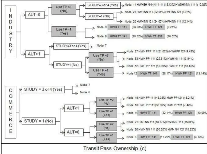
Among groups of individuals owning a transit pass (variable “Transit Pass Ownership”),
there is a predominance of transit usage TT (Figure 5 (c) - terminal nodes 9, 8 and 12 –
Industry; terminal nodes 10 and 8 – Commerce). Those people who do not own a transit pass
(terminal nodes 11, 21, 20 27, 53 and 52 – Industry; terminal node 19, 18, 21 and 20 –
Commerce) are more inclined towards the particular or non-motorized travel modes (NN,
NNN or PP).
Specific cases were observed, in both samples, of individuals who prefer to use transit for
distance to be covered (exceeding 15 km), travel costs will probably be lower than with car
usage (fixed tariff of transit - specifically for the SPMA). These cases are shown in terminal
nodes 12 (industry) and 10 (commerce).
Figure 5 - CART construction (c) Transit Pass Ownership influence
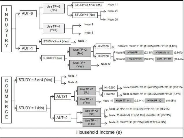
Individuals that have higher incomes frequently tend to use cars in the travel mode sequence.
For industrial workers, for example, the majority of individuals with a Household Income
greater than or equal to R$ 29701 (terminal node 27) use an automobile - HWH PP 111
(51.02%) and HWH PP 121 (4.43%). For commercial workers, a great number of individuals
with a Household Income greater than or equal to R$ 22602 (terminal node 19) also use cars
in the travel mode sequences HWH PP 111 (48.33%) and HWH PP 121 (13.21%) – Figure 6
(a).
1 1R$ (Real Brazilian) = 0.50 American Dollar; 2,970R$ = 1,485 U$ 2
Figure 6 - CART construction (a) Household Income influence.
For the industrial workers (Figure 6 (b)), land use variables (accumulated opportunities in the
industry sector until 5 km from the Home TZ (5 IND km); accumulated opportunities in the
industry sector until 10 km from the Home TZ (10 IND km); accumulated opportunities in the
industry sector until 15 km from the Home TZ (15 IND km)) exert significant influences on
the sequences of destinations.
In the case of industrial workers especially, individuals that live in traffic zones with few
accumulated job opportunities in their neighborhoods (IND 5 km < 3.22%, e.g., terminal node
8) tend to carry out longer trips related to work (HWH TT 141), see Figure 6 (b).
It is noted that only one of the land use variables in the sample of commercial workers was
selected (COM 5 km – Figure 6 (b)). In this case, the land use variable does not intervene
predominantly in destination sequence choice. This result is due to the geographic distribution
of commercial jobs. Commercial jobs are sufficiently dispersed, and there are no
Moreover, commercial workers more frequently perform short trips (111), which can be
explained on the basis of the geographic dispersion of commercial activities in the SPMA.
Individuals working in the commerce sector probably live near their work locations.
For commercial workers, the variable “Work” (Figure 6 (c)) influences the choice of the trip
purpose sequence. This variable is important due to sample characteristics; there is greater
number of autonomous workers in the commerce sector.
Figure 6 - CART construction (b) Land Use influence
The individuals that were selected in terminal nodes 20 and 21 possess some similar
characteristics and can be clearly distinguished for the independent variable “Work”. The
individuals that form node 20 are employees, while those who are part of node 21 are
autonomous workers. Members of the autonomous group generally do not have a need to
carry out daily trips related to work and can perform sequences unrelated to work activities.
In the exploratory stage of this work, results obtained the CART algorithms were analyzed.
The influences of some independent variables on trip sequences (activities, travel modes or
destinations) were verified. The important influence of the land use variable set in the
industrial worker sample was noted. This fact is accounted for by the geographic
concentration of jobs in the industry sector in the SPMA.
Considering public policy implications, we could note that is probably possible to change
work related trips choices, modifying the spatial arrangement of activities in the industrial and
tertiary sectors.
Figure 6 - CART construction (c) Work influence
The next stage of the study, Multiple Linear Regression (MLR), aimed to corroborate initial
conclusions and gain statistical insights. In the confirmatory stage, the parameters used to
prove the contribution of the independent variables in the accomplishment of travel patterns
5. Confirmatory analysis
In this research, the Multiple Linear Regression (MLR) application was associated with
CART application. In this confirmatory stage the following steps were accomplished:
(1) Discretization of independent variables; (2) representation of dependent variable;
(3) Correlation analysis for the independent variables; and (4) achievement of linear models
and discussions.
The categorization of independent variables was the first step. Each continuous variable was
divided into two classes (dummy variables) to reduce the eventual non-linearity between
independent and dependent variables. The corresponding values for the classes of the dummy
variables were obtained through CART application. Thus, for example, the continuous
variable IND 5km became a dummy variable with the following values: (a) 5 IND km < 3.2%
(0); (b) 5 IND km > 3.2% (1). This process was repeated for all independent variables
selected by the CART application and the values used for the data split.
The following example illustrates the representation of dependent variables:
(1) The individual 1 belonging to the industry sector workers sub-sample is considered;
(2) During the CART construction, individual 1 was classified in terminal node 8;
(3) People classified in terminal node 8 have a probability of 0.22 of carrying out the travel
pattern HWH TT 121, for example; and
(4) This probability is the value of the dependent variable “y”, corresponding to individual 1.
In this work the probability of the occurrence of ten travel patterns was considered for each
individual of the two sub-samples. The ten travel patterns considered were: HWH TT 141,
HWH TT 131, HWH TT 121, HWH TT 111, HWH PP 141, HWH PP 131, HWH PP 121,
HWH PP 111, HWH NN 121 and HWH NN 111. Thus, ten linear models for each sub-sample
were obtained (total of 20), where the dependent variables are the probabilities of the
An analysis of the correlations between all variables, including the independent variables
(dummy) and the dependent variables (numerical 0 to 1), was performed. If two independent
variables were detected to be highly correlated, the one that was less correlated with the
dependent variable was discarded. Table 2 shows each of the twenty linear models, the
coefficient values associated with each of the independent variables (parameters) and t
statistics and R2 values. Table 3 describes the independent dummy variables.
All twenty models obtained were considered acceptable, with values of R2 varying from 0.570
(model HWH PP 141 of the sample of commerce sector workers) to 0.893 (model HWH TT
121 of the sample of industry sector workers).
All independent variables were significant, with relatively high values of t-statistics.
Moreover, all the coefficient values (parameters) obtained were coherent. In the next
sub-section, the contributions of each variable for the accomplishment of the ten travel patterns for
the two sub-samples will be described.
5.1 Independent variable influence: The MLR models
Having at least one car in the household (value one for the variable “car ownership”- AUT),
results in a negative contribution to the accomplishment of travel patterns associated with
transit (TT) or non-motorized (NN or NNNN) travel mode sequences in both sub-samples.
HWH TT 141 (industry (-0.006); commerce (-0.002)); HWH TT 131 (industry (-0.019);
commerce (-0.029)); HWH TT 121 (industry (-0.038); commerce (-0.039)); HWH TT 111
(industry (-0.084); commerce (-0.059)); HWH NN 111 (industry (-0.133); commerce (-0.087))
Table 2 - Results of MLR Application
Intercept AUT TP HI Study Work IND 5km IND 10 km IND 15km COM 5 km R2
ß 0.261 -0.006 -0.109 -0.025 -0.048 -0.101
t 145.85 -9.81 -56.56 -9.09 -16.92 -54.71
ß 0.15 -0.019 -0.089 -0.03 -0.033 -0.046
t 254.43 -9.98 -106.77 -24.16 -34.29 -43.76
ß 0.227 -0.038 -0.099 -0.055 -0.061 -0.004
t 315.23 -47.78 -124.79 -48.2 -52.31 -5.52
ß 0.207 -0.084 -0.09 -0.058 -0.033 0.066
t 140.44 -52.62 -56.5 -22.33 -14.06 37.03
ß 0.047 0.024 0.099 -0.043 -0.011
t 50.86 26.38 71.000 -31.55 -12.61
ß -0.008 0.053 0.019 0.039 -0.025 0.008
t -19.86 94.71 41.41 30.91 -37.43 18.88
ß -0.005 0.068 0.027 0.031 -0.045
t -8.0 94.27 37.17 22.000 -41.88
ß -0.021 0.102 0.047 0.029 -0.045 0.02
t -22.68 101.94 47.3 22.14 -30.267 20.672
ß 0.077 -0.133 0.175 -0.77 -0.36 0.026
t 39.64 -61.78 81.37 -25.33 -11.26 12.69
ß 0.028 -0.024 0.044 -0.006 0.106
t 34.82 -52.22 85.76 -12.18 63.8
ß 0.199 -0.002 -0.132 -0.019 -0.107 -0.099 0.044
t 100.24 -28.74 -103.83 -15.29 -74.07 -9.13 23.33
ß 0.122 -0.029 -0.074 -0.021 -0.06 -0.008 0.028
t 107.85 -45.97 -101.71 -17.96 -75.52 -13.19 25.55
ß 0.173 -0.039 -0.107 -0.026 -0.082 -0.017 0.039
t 101.54 -40.55 -98.18 -15.89 -68.18 -18.01 24
ß 0.169 -0.059 -0.077 -0.033 -0.076 -0.013 0.029
t 144.07 -71.01 -81.16 -17.72 -70.84 -15.09 21.8
ß 0.007 0.035 0.025 0.045 -0.029 0.002 0.004
t 5.06 39.48 28.92 39.14 -29.88 2.21 3.95
ß -0.005 0.043 0.02 0.034 -0.028 0.001 0.002
t -6.28 76.68 39.85 30.18 -50.91 2.73 3.77
ß -0.006 0.052 0.039 0.03 -0.049 -0.002
t -6.98 64.5 41.87 34.11 -47.53 -3.07
ß -0.033 0.096 0.065 0.029 -0.063 0.005 0.008
t -14.37 74.68 44.33 24.4 -38.08 3.55 3.74
ß 0.114 -0.087 0.149 -0.026 -0.043 -0.012 -0.026
t 44.17 -59.56 89.38 -16.52 -22.91 -8.16 -10.74
ß 0.025 -0.034 0.055 -0.004 0.155 -0.023
t 33 -59.42 90.76 -14.65 75.66 -12.79
0.713 0.765 0.776 0.791 0.57 0.758 0.738 0.746 0.868 0.846 0.784 0.713 0.783 0.794 0.725 0.834 0.893 0.718 0.784 0.839 3 4 5 6 7 8
HWH TT 141
C o m m e rc e
1 HWH TT 141
2 3 4 In d u st ry 1 2 9 6,043 10 9 10 4,102
HWH PP 131
HWH PP 121
5
6
7
8
HWHSH NNNN 1111 HWH PP 111
HWH NN 111
HWHSH NNNN 1111
HWH TT 131
HWH TT 121
HWH TT 111 Linear Models
HWH PP 141
HWH PP 131
HWH PP 121
HWH PP 111
HWH NN 111 HWH TT 131
HWH TT 121
HWH TT 111
HWH PP 141
Individuals that have cars in the household predominantly use automobiles (PP) for traveling
between the locations of their activities. Thus, the coefficients for the variable AUT are
positive for the travel patterns with car usage: HWH PP 141 (industry (0.047); commerce
(0.035)); HWH PP 131 (industry (0.053); commerce (0.043)); HWH PP 121 (industry
(0.068); commerce (0.052)); HWH PP 111 (industry (0.102); commerce (0.096)).
Table 3 – Dummy independente variables
Description code
car ownership AUT AUT = 0 AUT >=1
Transit Pass Ownership TP TP=1 (use) TP=2 (do not use)
HI (IND) HI (IND) < 2970 HI (IND) > 2970 HI (COM) HI (COM) < 2260 HI (COM) > 2260
Study STUDY STUDY=1(No) STUDY>1 (Yes)
work WORK WORK = 1 (Employee) WORK=2 (Autonomous)
accumulated opportunities in the industry sector until
5 km from the Home TZ
accumulated opportunities in the industry sector until
10 km from the Home TZ
accumulated opportunities in the industry sector until
15 km from the Home TZ
accumulated opportunities in the commerce sector until
5 km from the Home TZ
IND 15 km IND 15 km < 32.3 IND 15 km > 32.3
COM 5 km COM 5 KM < 0.008 COM 5 km > 0.008 IND 5 km IND 5 km < 3.2 IND 5 km > 3.2
IND 10 km IND 10 km < 15.6 IND 10 km > 15.6
values
Household Income
0 1
Dummy variables
In the models for automobile usage (HWH PP 141, HWH PP 131, HWH PP 121 and HWH
PP 111), the contribution of the variable “AUT” is greater for shorter travel distances, such as
HWH PP 111. Frequently, people choose driving short distances instead walking when they
have cars in the household.
The results obtained through CART application suggest that individuals that are studying (and
are workers in the industry or commerce sector) perform activity sequences related to work
and school - (variable –“Study”).
In such a way, individuals who are studying and working (variable “Study” equal to unity) accomplish travel patterns with trip purposes related to Work and School (HWHSH). A
positive contribution in the two samples for this variable in the model HWHSH NNNN 11111
People who do not use TP (value one for the variable “Transit Pass Ownership”)
predominantly do not use transit in the travel mode sequence. Thus, the coefficients for this
variable are highly negative in the models with transit usage: HWH TT 141 (industry (-
0.109); commerce (- 0.132)); HWH TT 131 (industry (- 0.089); commerce (- 0.074)); HWH
TT 121 (industry (- 0.099); commerce (- 0.107)); HWH TT 111 (industry (- 0.090); commerce
(- 0.077)).
The importance of this variable in choice of travel mode, especially related to transit usage, is
evident. The estimated coefficient values for this variable confirm the previous results
obtained using the CART application.
Positive estimated values of the coefficients are found in the case of the models associated
with automobile or walking choices (PP and NN): HWH PP 141 (industry (0.024); commerce
(0.025)); HWH PP 131 (industry (0.019); commerce (0.020)); HWH PP 121 (industry
(0.027); commerce (0.039)); HWH PP 111 (industry (0.047); commerce (0.065)); HWH NN
111 (industry (0.175); commerce (0.149)).
As noted previously, individuals with high Household Incomes frequently use cars in their
trip sequences. Thus, Household Incomes greater than or equal to R$ 2970 (industry sector
workers) or R$ 2260 (commerce sector workers) - (variable ”Household Income”- HI equal
to unity) contribute negatively to the fulfillment of the travel patterns involving transit and
non-motorized usage (TT or NN): HWH TT 141 (industry (- 0.025); commerce (- 0.019));
HWH TT 131 (industry (- 0.030); commerce (- 0.021)); HWH TT 121 (industry (- 0.055);
commerce (- 0.026)); HWH TT 111 (industry (- 0.058); commerce (- 0.033)); HWH NN 111
(industry (- 0.770); commerce (- 0.026)).
Otherwise, positive values for the coefficients associated with the models (travel patterns)
with car usage (PP) were observed: HWH PP 141 (industry (0.099); commerce (0.045));
HWH PP 131 (industry (0.039); commerce (0.034)); HWH PP 121 (industry (0.031);
commerce (0.030)); HWH PP 111 (industry (0.029); commerce (0.029)).
conclusion that people with high incomes not only use predominantly automobiles but also
carry out longer trips.
The high value for the “Land Use” variable in the model HWH TT 141 (industry sector
workers) indicates the importance of this variable in destination choices. Individuals that live
in TZs with high accumulated industry opportunities (IND 5 km > 3.22%) are more disposed
to carry out short trips. Thus, if the variable “IND 5km” assumes value one (5 IND km >
3.22%), this strongly and negatively influences the accomplishment of the travel pattern
HWH TT 141 (travel distances above of 15 km – Destination/travel distance sequences 141).
In the model pattern HWH TT 131 (industry sector workers), if the variable IND 10km has a
value of 1 (10 IND km > 15.6%) there is a negative influence (-0.046) on the fulfillment of
the travel pattern HWH TT 131. Individuals that live in TZs with high accumulated industry
opportunities until 10 km from the centroid predominantly carry out travel distances shorter
than 10 km and not between 10 and 15 km (“131”).
In the sample of commerce sector workers, smaller influences of the land use variables were
observed. The biggest value of the parameter associated with the land use variable was 0.044 for the variable “COM 5 km” in model HWH TT 141. This confirms that the influence of the land use for the case of commerce sector workers is not strong.
Conclusion
This research confirmed two main hypotheses: (1) it is possible to find relationships between
urban travel patterns (dependent variable) and socioeconomic characteristics, land use and
out-of-home activity participation; and (2) the different spatial distributions of economic
activities (commercial and industrial) in the urban environment influence the travel of
commerce or industry sector workers.
In the first and second parts of this article (exploratory and confirmatory analysis,
respectively), relations were found between variables using CART algorithms and confirmed
through the measurement of the statistical significances of the independent variables using
This study has some limitations related to the methodology application, such as: (1) constraint
of travel patterns number by the statistical package used (S-PLUS 6.1), (2) Lack of data
related to the spatial distribution for other activities beyond industrial and commercial, (3) use
of centroid distances of Traffic Zones.
The results obtained allowed for detailed analysis of the influence of the three variable groups
on travel patterns: (1) socioeconomic variables (Household Income, Transit Pass Ownership ,
Car-ownership) appear to affect the travel mode sequence used for trips; (2) activity
participation (Study, Work) is important for the trip purpose sequence; and (3) land use
variables (accumulated proportion of jobs by distance buffers starting from the residence zone
centroid) has a significant influence on the sequence of chosen destinations. It is expected that
the results of this research can be used to represent the level of activities and their geographic
distribution in the urban configuration (land use variables) and to determine the influence of
such variables on commerce and industry sector worker travel.
The SPMA has experienced an increase in jobs in the tertiary sector in recent years, to the
detriment of jobs in the industry sector. These changes in the job market can modify travel
patterns. In this work, travel behavior differences between industry and the commerce sector
workers, governed by the geographic distribution of such activities, are investigated.
Acknowledgments
This work was partially supported by the Fundação para Ciência e Tecnologia (FCT). The
authors are grateful to Companhia do Metropolitano de São Paulo (METRÔ-SP) for the data
References
Arentze, T., Hofman V, Mourik van, H. and Timmermans, H. (2000). ALBATROSS: Multiagent, Rule-Based Model of Activity Pattern Decisions. In Transportation Research Record: Journal of the Transportation Research Board, No 1706, Transportation Research Board of the National Academies, Washington, D.C, pp. 136-144.
Balasubramaniam, C. and Goulias, K. (1999) Exploratory longitudinal analysis of solo and joint trip making. 78th Annual Meeting of Transportation Research Board. Compendium of Papers CD-ROM, 1999, Washington, D.C.
Bhat, C.R. and Singh, S.K (2000) A comprehensive daily activity-travel generation model system for workers. Transportation Research Part A, v.34, pp.1-22.
Bhat C.R. and Koppelman , F.S (1991) A conceptual framework of individual activity program generation. Transportation Research Part A, v. 27, 1991, pp.433-446.
Breiman, L., Friedman J.H, Olshen, R.A. and Stone, C.J. (1984). Classification and Regression Trees. Wadsworth International Group, California.
Bowman, J.L. and Ben-Akiva, M.E. (2000) Activity-based disaggregate travel demand model system with activity schedules. Transportation Research Part A, v.35, pp.1-28.
Cervero, R. and Radisch, M.E. (1996). Pedestrian versus automobile oriented neighborhoods. Transport Policy, v.3, pp.127-141.
Ewing, R. (1995) Beyond density, mode choice, and single-purpose trips. Transportation Quarterly, v.49, pp. 16-23.
Golob, T.F and Mcnally, M. (1997) A model of activity participation and travel interactions between household heads. Transportation Research Part B, v.31, pp.177-194.
IBGE – INSTITUTO BRASILEIRO DE GEOGRAFIA E ESTATÍSTICA. Censo Demográfico 2000. Características urbanísticas em torno dos domicílios. Rio de Janeiro: Ministério do Planejamento, Orçamento e Gestão, 2000. In portuguese.
Kitamura, R., Mokhtarian, P.L and Laidet, L. (1997). A micro-analysis of land use and travel in five neighborhoods in the San Francisco Bay Area., Transportation, n. 24, pp. 125-158.
Kwan M. (2000) Interactive revisualization of activity-travel patterns using three-dimensional geographical information systems: a methodological exploration with a large data set. Transportation Research Part C, v.8, pp.185-203.
Lu, X. and Pas, E.I. (1999). Socio-demographics, activity participation and travel behavior. Transportation Research Part A, v.33, pp.1-18.
Mcguckin, N. and Murakami, E. (1999) Examining trip-chaining behavior: Comparison of travel by men and women. In Transportation Research Record: Journal of the Transportation Research Board, No 1693, Transportation Research Board of the National Academies, Washington, D.C, pp. 79-85.
METRO (2000) Pesquisa Origem Destino 1997 – Região Metropolitana de São Paulo: Síntese das informações. In portuguese.
Piramuthu, S. (2008) Input data for decision trees. Expert Systems with applications, v.34, pp. 1220-1226.
Simma, A. and Axhausen, K.W. (2001) Within household allocation of travel: the case of upper Austria. In Transportation Research Record: Journal of the Transportation Research Board, No 1752, Transportation Research Board of the National Academies, Washington, D.C, pp. 69-75.
Srinivasan, K.K. and Athuru, S.R. (2005). Analysis of within-household effects and between household differences in maintenance activity allocation. Transportation, v.32, pp.495-521.
Strambi, O., Vespucci, K.M and van de Bilt, K. (2004) Analysis of the evolution of classes of individual patterns and their relation to socio-demographic and economic variables. 83rd Annual Meeting of Transportation Research Board. Compendium of Papers CD-ROM, Washington, D.C.