eig book 2ndEd Numerical Methods for Large Eigenvalue Problems

(1)

. . .. .. .. .. .. . . .. .. .. .. .. . . . .. .. . .. .. .. . . . .. . . . .. . . . . . . . .. .. . .. .. .. . .. . . .. . .. .. .. . . . .. .. ... . ... . ... . ... . . ... . ... . ... . ... . . ... . ... . . ... . ... . . ... . ... . . .. ... . . ... . . .. ... . . ... .. .. ... . . . . ... . . .. ... . . ... . . ... . . . . ... . . ... . . .. ... . . ... . . ... . . .. ... . . ... . . ... . . ... . . . . ... . . ... . . ... . . ... . . ... . . .. ... . . ... . . . . . . . . .. . . . . . . . . . . . . . . .. . . . . . . . . . . . . . . . . . . . . . . . . . . . . . . . . . . . . . . . . . . . . . . . . . . . . . . . . . . . . . . . . . . . . . . . . . . . . . . . . . . . . . . . . . . . . . . . . . .

NUMERICAL METHODS FOR LARGE

EIGENVALUE PROBLEMS

✞ ✝ ☎ ✆

Second edition

Yousef Saad

(2)

(3)

Preface to the Classics Edition

This is a revised edition of a book which appeared close to two decades ago. Someone scrutinizing how the field has evolved in these two decades will make two interesting observations. On the one hand the observer will be struck by the staggering number of new developments in numerical linear algebra during this period. The field has evolved in all directions: theory, algorithms, software, and novel applications. Two decades ago there was essentially no publically available software for large eigenvalue problems. Today one has a flurry to choose from and the activity in software development does not seem to be abating. A number of new algorithms appeared in this period as well. I can mention at the outset the Jacobi-Davidson algorithm and the idea of implicit restarts, both discussed in this book, but there are a few others. The most interesting development to the numeri-cal analyst may be the expansion of the realm of eigenvalue techniques into newer and more challenging applications. Or perhaps, the more correct observation is that these applications were always there, but they were not as widely appreciated or understood by numerical analysts, or were not fully developed due to lack of software.

The second observation to be made when comparing the state of the field now and two decades ago is that at the same time the basic tools used to compute spec-tra have essentially not changed much: Krylov subspaces are still omnipresent. On the whole, the new methods that have been developed consist of enhance-ments to these basic methods, sometimes major, in the form of preconditioners, or other variations. One might say that the field has evolved even more from gaining maturity than from the few important developments which took place. This ma-turity has been brought about by the development of practical algorithms and by software. Therefore, synergetic forces played a major role: new algorithms, en-hancements, and software packages were developed which enabled new interest from practitioners, which in turn sparkled demand and additional interest from the algorithm developers.

In light of this observation, I have grouped the 10 chapters of the first edition into three categories. In the first group are those chapters that are of a theoreti-cal nature (Chapters 1, 3, and 9). These have undergone small changes such as correcting errors, improving the style, and adding references.

The second group includes a few chapters that describe basic algorithms or concepts – for example subspace iteration (Chapter 5) or the tools of spectral

(8)

approximation (Chapter 4). These have been left unchanged or have received small updates. Chapters 2 and 10 are also in this group which then consists of Chapters 2, 4, 5, and 10.

Chapters in the third group (chapters 6 to 8) underwent the biggest changes. These describe algorithms and their implementations. Chapters 7 and 8 of the first edition contained a mix of topics some of which are less important today, and so some reorganization was needed. I preferred to shorten or reorganize the discussion of some of these topics rather than remove them altogether, because most are not covered in other books. At the same time it was necessary to add a few sections on topics of more recent interest. These include the implicit restart techniques (inlcuded in Chapter 7) and the Jacobi-Davidson method (included as part of Chapter 7 on preconditioning techniques). A section on AMLS (Auto-matic Multi-Level Substructuring) which has had excellent success in Structural Engineering has also been included with a goal to link it to other known methods. Problems were left unchanged from the earlier edition, but the Notes and ref-erences sections ending each chapter were systematically updated. Some notation has also been altered from the previous edition to reflect more common usage. For example, the term “null space” has been substituted to less common term “kernel.” An on-line version of this book, along with a few resources such as tutorials, and MATLAB scripts, is posted on my web site; see:

http://www.siam.org/books/cl66

Finally, I am indebted to the National Science Foundation and to the Depart-ment of Energy for their support of my research throughout the years.

Yousef Saad

(9)

Preface

Matrix eigenvalue problems arise in a large number of disciplines of sciences and engineering. They constitute the basic tool used in designing buildings, bridges, and turbines, that are resistent to vibrations. They allow to model queueing net-works, and to analyze stability of electrical networks or fluid flow. They also allow the scientist to understand local physical phenonema or to study bifurcation pat-terns in dynamical systems. In fact the writing of this book was motivated mostly by the second class of problems.

Several books dealing with numerical methods for solving eigenvalue prob-lems involving symmetric (or Hermitian) matrices have been written and there are a few software packages both public and commercial available. The book by Parlett [148] is an excellent treatise of the problem. Despite a rather strong demand by engineers and scientists there is little written on nonsymmetric prob-lems and even less is available in terms of software. The 1965 book by Wilkinson [222] still constitutes an important reference. Certainly, science has evolved since the writing of Wilkinson’s book and so has the computational environment and the demand for solving large matrix problems. Problems are becoming larger and more complicated while at the same time computers are able to deliver ever higher performances. This means in particular that methods that were deemed too demanding yesterday are now in the realm of the achievable. I hope that this book will be a small step in bridging the gap between the literature on what is avail-able in the symmetric case and the nonsymmetric case. Both the Hermitian and the non-Hermitian case are covered, although non-Hermitian problems are given more emphasis.

This book attempts to achieve a good balance between theory and practice. I should comment that the theory is especially important in the nonsymmetric case. In essence what differentiates the Hermitian from the non-Hermitian eigenvalue problem is that in the first case we can always manage to compute an approxi-mation whereas there are nonsymmetric problems that can be arbitrarily difficult to solve and can essentially make any algorithm fail. Stated more rigorously, the eigenvalue of a Hermitian matrix is always well-conditioned whereas this is not true for nonsymmetric matrices. On the practical side, I tried to give a general view of algorithms and tools that have proved efficient. Many of the algorithms described correspond to actual implementations of research software and have been tested on realistic problems. I have tried to convey our experience from the

(10)

practice in using these techniques.

As a result of the partial emphasis on theory, there are a few chapters that may be found hard to digest for readers inexperienced with linear algebra. These are Chapter III and to some extent, a small part of Chapter IV. Fortunately, Chap-ter III is basically independent of the rest of the book. The minimal background needed to use the algorithmic part of the book, namely Chapters IV through VIII, is calculus and linear algebra at the undergraduate level. The book has been used twice to teach a special topics course; once in a Mathematics department and once in a Computer Science department. In a quarter period representing roughly 12 weeks of 2.5 hours lecture per week, Chapter I, III, and IV, to VI have been cov-ered without much difficulty. In a semester period, 18 weeks of 2.5 hours lecture weekly, all chapters can be covered with various degrees of depth. Chapters II and X need not be treated in class and can be given as remedial reading.

(11)

BACKGROUND IN MATRIX THEORY

AND LINEAR ALGEBRA

This chapter reviews basic matrix theory and introduces some of the elementary notation used throughout the book. Matrices are objects that represent linear map-pings between vector spaces. The notions that will be predominantly used in this book are very intimately related to these linear mappings and it is possible to discuss eigenvalues of linear operators without ever mentioning their matrix representations. However, to the numerical analyst, or the engineer, any theory that would be de-veloped in this manner would be insufficient in that it will not be of much help in developing or understanding computational algorithms. The abstraction of linear mappings on vector spaces does however provide very concise definitions and some important theorems.

1.1 Matrices

When dealing with eigenvalues it is more convenient, if not more relevant, to manipulate complex matrices rather than real matrices. A complexm×nmatrix

Ais anm×narray of complex numbers

aij, i= 1, . . . , m, j= 1, . . . , n.

The set of allm×nmatrices is a complex vector space denoted byCm×n_{. The} main operations with matrices are the following:

• Addition:C=A+B,whereA, BandCare matrices of sizem×nand

cij =aij+bij , i= 1,2, . . . m, j= 1,2, . . . n.

• Multiplication by a scalar:C=αA,wherecij =α aij.

• Multiplication by another matrix:

C=AB,

(12)

whereA∈Cm×n_{, B}_∈_Cn×p_{, C} _∈_Cm×p_,_and cij =

n X k=1

aikbkj.

A notation that is often used is that of column vectors and row vectors. The column vector a.j is the vector consisting of thej-th column ofA, i.e., a.j = (aij)i=1,...,m. Similarly we will use the notationai.to denote thei-th row of the

matrixA. For example, we may write that

A= (a.1, a.2, . . . , a.n) .

or

A=

    

a1. a2. . . am.

    

The transpose of a matrixAinCm×nis a matrixCinCn×mwhose elements are defined bycij =aji, i= 1, . . . , n, j= 1, . . . , m. The transpose of a matrixA

is denoted byAT_{. It is more relevant in eigenvalue problems to use the transpose}

conjugate matrix denoted byAH_{and defined by} AH = ¯AT =AT

in which the bar denotes the (element-wise) complex conjugation.

Finally, we should recall that matrices are strongly related to linear mappings between vector spaces of finite dimension. They are in fact representations of these transformations with respect to two given bases; one for the initial vector space and the other for the image vector space.

1.2 Square Matrices and Eigenvalues

A matrix belonging toCn×n _{is said to be square. Some notions are only defined}

for square matrices. A square matrix which is very important is the identity matrix

I={δij}i,j=1,...,n

whereδijis the Kronecker symbol. The identity matrix satisfies the equalityAI=

IA=Afor every matrixAof sizen. The inverse of a matrix, when it exists, is a matrixCsuch thatCA=AC =I. The inverse ofAis denoted byA−1_.

The determinant of a matrix may be defined in several ways. For simplicity we adopt here the following recursive definition. The determinant of a1×1matrix

(a)is defined as the scalara. Then the determinant of ann×nmatrix is given by

det(A) =

n X j=1

(13)

whereA1jis an(n−1)×(n−1)matrix obtained by deleting the 1-st row and thej−thcolumn ofA. The determinant of a matrix determines whether or not a matrix is singular sinceAis singular if and only if its determinant is zero. We have the following simple properties:

• det(AB) = det(BA),

• det(AT_{) = det(}_A₎_, • det(αA) =αn_det(_A₎_, • det( ¯A) = det(A),

• det(I) = 1.

From the above definition of the determinant it can be shown by induction that the function that maps a given complex valueλto the valuepA(λ) = det(A−λI)

is a polynomial of degreen(Problem P-1.6). This is referred to as the character-istic polynomial of the matrixA.

Definition 1.1 A complex scalarλis called an eigenvalue of the square matrix

Aif there exists a nonzero vectoruofCnsuch thatAu = λu. The vectoruis called an eigenvector ofAassociated withλ. The set of all the eigenvalues ofA

is referred to as the spectrum ofAand is denoted byΛ(A).

An eigenvalue ofAis a root of the characteristic polynomial. Indeedλis an eigenvalue ofAiffdet(A−λI) ≡pA(λ) = 0. So there are at mostndistinct eigenvalues. The maximum modulus of the eigenvalues is called spectral radius and is denoted byρ(A):

ρ(A) = max

λ∈Λ(A) |λ|.

The trace of a matrix is equal to the sum of all its diagonal elements,

tr(A) =

n X i=1

aii.

It can be easily shown that this is also equal to the sum of its eigenvalues counted with their multiplicities as roots of the characteristic polynomial.

Proposition 1.1 Ifλis an eigenvalue ofAthen¯λis an eigenvalue ofAH_{. An}

eigenvectorvofAH_{associated with the eigenvalue}_λ_¯_{is called left eigenvector of} A.

When a distinction is necessary, an eigenvector ofAis often called a right eigen-vector. Thus the eigenvalueλand the right and left eigenvectors,uandv,satisfy the relations

Au=λu , vHA=λvH

or, equivalently,

(14)

1.3 Types of Matrices

The properties of eigenvalues and eigenvectors of square matrices will sometimes depend on special properties of the matrix A. For example, the eigenvalues or eigenvectors of the following types of matrices will all have some special proper-ties.

• Symmetric matrices: AT ₌_A_; • Hermitian matrices: AH ₌_A_; • Skew-symmetric matrices: AT ₌₋_A_; • Skew-Hermitian matrices: AH₌₋_A_; • Normal matrices: AH_A₌_AAH_;

• Nonnegative matrices: aij ≥ 0, i, j = 1, . . . , n(similar definition for nonpositive, positive, and negative matrices);

• Unitary matrices: Q ∈ Cn×nandQH_Q₌_I_.

It is worth noting that a unitary matrixQis a matrix whose inverse is its transpose conjugateQH. Often, a matrixQsuch that QHQis diagonal (not necessarily square) is called orthogonal.

1.3.1 Matrices with Special Srtuctures

Some matrices have particular structures that are often convenient for computa-tional purposes and play important roles in numerical analysis. The following list though incomplete, gives an idea of the most important special matrices arising in applications and algorithms. They are mostly defined for square matrices.

• Diagonal matrices: aij = 0 for j 6= i. Notation for square diagonal matrices:

A= diag (a11, a22, . . . , ann). • Upper triangular matrices:aij = 0fori > j.

• Lower triangular matrices:aij = 0fori < j.

• Upper bidiagonal matrices:aij= 0forj 6=iorj 6=i+ 1.

• Lower bidiagonal matrices:aij= 0forj 6=iorj 6=i−1.

• Tridiagonal matrices: aij = 0for any pairi, jsuch that_|j−i|>1. Nota-tion:

(15)

• Banded matrices: there exist two integers mlandmu such thataij 6= 0

only ifi−ml ≤ j ≤ i+mu. The numberml+mu + 1is called the bandwidth ofA.

• Upper Hessenberg matrices: aij = 0for any pairi, jsuch thati > j+ 1. One can define lower Hessenberg matrices similarly.

• Outer product matrices:A=uvH_,_{where both}_u_and_v_{are vectors.} • Permutation matrices: the columns ofAare a permutation of the columns

of the identity matrix.

• Block diagonal matrices: generalizes the diagonal matrix by replacing each diagonal entry by a matrix. Notation:

A= diag (A11, A22, . . . , Ann).

• Block tri-diagonal matrices: generalizes the tri-diagonal matrix by replac-ing each nonzero entry by a square matrix. Notation:

A= tridiag (Ai,i−1, Aii, Ai,i+1).

The above properties emphasize structure, i.e., positions of the nonzero ele-ments with respect to the zeros, and assume that there are many zero eleele-ments or that the matrix is of low rank. No such assumption is made for, say, orthogonal or symmetric matrices.

1.3.2 Special Matrices

A number of matrices which appear in applications have even more special struc-tures than the ones seen in the previous subsection. These are typically dense matrices, but their entries depend on fewer parameters thann2_.

Thus, Toeplitz matrices are matrices whose entries are constant along diago-nals. A5×5Toeplitz matrix will be as follows:

T =

    

t0 t1 t2 t3 t4

t−1 t0 t1 t2 t3 t−2 t−1 t0 t1 t2 t−3 t−2 t−1 t0 t1 t−4 t−3 t−2 t−1 t0

     ,

wheret−4, t−3,· · · , t3, t4are parameters. The entries ofAare such thatai,i+k=

tk, a constant depending only onk, fork =−(m−1),−(m−2),_{· · ·} ,0,1,2,

(16)

Similarly, the entries of Hankel matrices are constant along anti-diagonals:

H =



   

h1 h2 h3 h4 h5 h2 h3 h4 h5 h6 h3 h4 h5 h6 h7 h4 h5 h6 h7 h8 h5 h6 h7 h8 h9



    .

The entries ofAare such thatai,k+1−i =hk, a constant which depends only on k, fork= 1,2,· · · , m+n−1. Again, indices(i, k+ 1−i)falling outside the valid range of indices forAare ignored. Hankel matrices are determined by the

m+n−1valueshk.

A special case of Toplitz matrices is that of Circulant matrices which are defined bynparametersη1, η2,· · · , ηn. In a circulant matrix, the entries in a row are cyclically right-shifted to form next row as is shown in the following5×5

example:

C=



   

η1 η2 η3 η4 η5 η5 η1 η2 η3 η4 η4 η5 η1 η2 η3 η3 η4 η5 η1 η2 η2 η3 η4 η5 η1



   

An important practical characteristic of these special matrices, is that fast algorithms can often be devised for them. For example, one could hope that a Toeplitz linear system can be solved faster than in the standardO(n3)operations normally required, perhaps in ordern2 _{operations. This is indeed the case, see}

[77] for details.

Circulant matrices are strongly connected to the discrete Fourier transform. The eigenvectors of a circulant matrix of a given size are the columns of the dis-crete Fourier transform matrix of sizen:

Fn= (fjk) with fjk= 1/√Ne−2jkπi/n,for0≤j, k < n.

More specifically, it can be shown that a circulant matrixCis of the form

C=Fndiag (Fnv)Fn−1

whereFnvis the discrete Fourier transform of the vectorv = [η1, η2,· · ·, ηn]T

(the first column of C). For this reason matrix-vector products with circulant matrices can be performed inO(nlog2n)operations via Fast Fourier Transforms

(FFTs) instead of the standardO(n2₎_operations.

1.4 Vector Inner Products and Norms

We define the Hermitian inner product of the two vectorsx = (xi)i=1,...,mand y= (yi)i=1,...,mofCmas the complex number

(x, y) =

m X i=1

(17)

which is often rewritten in matrix notation as

(x, y) =yHx.

A vector norm onCm is a real-valued function onCm, which satisfies the following three conditions,

kxk ≥0 ∀x, and _kxk= 0iffx= 0;

kαxk=|α|kxk, ∀x∈Cm_, _∀_α_∈C_; kx+yk ≤ kxk+kyk, ∀x, y∈Cm_.

Associated with the inner product (1.1) is the Euclidean norm of a complex vector defined by

kxk2= (x, x)1/2.

A fundamental additional property in matrix computations is the simple relation

(Ax, y) = (x, AHy) ∀x∈Cn_{, y}_∈Cm _(1.2) the proof of which is straightforward. The following proposition is a consequence of the above equality.

Proposition 1.2 Unitary matrices preserve the Hermitian inner product, i.e.,

(Qx, Qy) = (x, y)

for any unitary matrixQ.

Proof. Indeed(Qx, Qy) = (x, QH_Qy_{) = (}_{x, y}₎_.

In particular a unitary matrix preserves the 2-norm metric, i.e., it is isometric with respect to the 2-norm.

The most commonly used vector norms in numerical linear algebra are special cases of the H¨older norms defined as follows forp≥1

kxkp=

n X i=1

|xi|p !1/p

. (1.3)

It can be shown that these do indeed define norms forp≥1. Note that the limit of

kxkpwhenptends to infinity exists and is equal to the maximum modulus of the

xi’s. This defines a norm denoted by_k.k∞. The casesp= 1, p= 2,andp=∞ lead to the most important norms in practice,

kxk1=|x1|+|x2|+· · ·+|xn| kxk2=

|x1|2+|x2|2+· · ·+|xn|21/2 kxk∞= max

(18)

A very important relation satisfied by the 2-norm is the so-called Cauchy-Schwarz inequality:

|(x, y)| ≤ kxk2kyk2.

This is a special case of the H¨older inequality:

|(x, y)| ≤ kxkpkykq,

for any pairp, qsuch that1/p+ 1/q= 1andp≥1.

1.5 Matrix Norms

For a general matrixAinCm×n _{we define a special set of norms of matrices as}

follows

kAkpq= max

x∈Cn_{, x}₆₌₀

kAxkp

kxkq . (1.4)

We say that the norms_k.kpqare induced by the two normsk.kpandk.kq. These

satisfy the usual properties of norms, i.e.,

kAk ≥0 ∀A ∈Cm×n and _kAk= 0 iff A= 0 ;

kαAk=|α|kAk,∀A ∈Cm×n_, _∀_α_∈C_; kA+Bk ≤ kAk+kBk, ∀A, B ∈Cm×n_.

Again the most important cases are the ones associated with the casesp, q= 1,2,∞. The caseq=pis of particular interest and the associated norm_k.kpqis

simply denoted by_k.kp.

A fundamental property of these norms is that

kABkp≤ kAkpkBkp,

which is an immediate consequence of the definition (1.4). Matrix norms that satisfy the above property are sometimes called consistent. As a result of the above inequality, for example, we have that for any square matrixA,and for any non-negative integerk,

kAkkp≤ kAkkp,

which implies in particular that the matrix Ak _{converges to zero as} _k _{goes to}

infinity, if any of itsp-norms is less than 1. The Frobenius norm of a matrix is defined by

kAkF = 

 n X j=1

m X i=1

|aij|2 

 1/2

. (1.5)

(19)

by a pair of vector norms, i.e., it is not derived from a formula of the form (1.4), see Problem P-1.3. However, it does not satisfy some of the other properties of thep-norms. For example, the Frobenius norm of the identity matrix is not unity. To avoid these difficulties, we will only use the term matrix norm for a norm that is induced by two norms as in the definition (1.4). Thus, we will not consider the Frobenius norm to be a proper matrix norm, according to our conventions, even though it is consistent.

It can be shown that the norms of matrices defined above satisfy the following equalities which provide alternative definitions that are easier to use in practice.

kAk1= max j=1,..,n

m X i=1

|aij|; (1.6)

kAk∞= max

i=1,..,m n X j=1

|aij|; (1.7)

kAk2=

ρ(AHA)1/2

=

ρ(AAH)1/2

; (1.8)

kAkF =

tr(AHA)1/2

=

tr(AAH)1/2

. (1.9)

It will be shown in Section 5 that the eigenvalues ofAH_A_{are nonnegative.}

Their square roots are called singular values ofA and are denoted by σi, i = 1, . . . , n. Thus, relation (1.8) shows that_kAk2is equal toσ1,the largest singular

value ofA.

Example 1.1. From the above properties, it is clear that the spectral radius

ρ(A)is equal to the 2-norm of a matrix when the matrix is Hermitian. How-ever, it is not a matrix norm in general. For example, the first property of norms is not satisfied, since for

A=

0 1 0 0

we haveρ(A) = 0whileA 6= 0. The triangle inequality is also not satisfied for the pairA, BwhereAis defined above andB=AT_{. Indeed,}

ρ(A+B) = 1 while ρ(A) +ρ(B) = 0.

1.6 Subspaces

A subspace ofCm _{is a subset of}_Cm_{that is also a complex vector space. The}

set of all linear combinations of a set of vectorsG={a1, a2, ..., aq}ofCm_{is a}

vector subspace called the linear span ofG,

span{G} = span{a1, a2, . . . , aq}

=

(

z ∈Cm_|_z₌ q X i=1

αiai; {α}i=1,...,q ∈Cq )

(20)

If theai’s are linearly independent, then each vector ofspan{G}admits a unique expression as a linear combination of theai’s. The setGis then called a basis of the subspacespan{G}.

Given two vector subspacesS1andS2,their sumSis a subspace defined as the set of all vectors that are equal to the sum of a vector ofS1and a vector ofS2. The intersection of two subspaces is also a subspace. If the intersection ofS1and

S2is reduced to_{0}then the sum ofS1andS2 is called their direct sum and is denoted byS=S1L_S2_{. When}_S_{is equal to}_Cm_{then every vector}_x_of_Cm_can

be decomposed in a unique way as the sum of an elementx1ofS1and an element

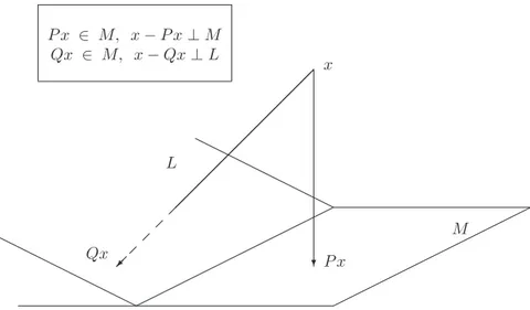
x2 ofS2. In this situation, we clearly have dim (S1) + dim (S2) = m. The transformationPthat mapsxintox1is a linear transformation that is idempotent (P2₌_P _{). It is called a projector, onto}_S1_along_S2_.

Two important subspaces that are associated with a matrixAofCm×nare its range, defined by

Ran(A) ={Ax|x∈Cn_}_, (1.10)

and its null space or kernel:

Null(A) ={x∈Cn_|_Ax_{= 0}_}_.

The range of A, a subspace of Cm, is clearly equal to the linear span of its columns. The column rank of a matrix is equal to the dimension of the range ofA, i.e., to the number of linearly independent columns. An important property of matrices is that the column rank of a matrix is equal to its row rank, the number of linearly independent rows ofA. This common number is the rank ofAand it clearly satisfies the inequality

rank(A)≤min{m, n}. (1.11)

A matrix inCm×n is of full rank when its rank is equal to the smallest ofnand

m, i.e., when equality is achieved in (1.11).

A fundamental result of linear algebra is stated by the following relation

Cm_{= Ran(}_A₎_⊕_Null(_AT₎_. _(1.12) The same result applied to the transpose ofAyields:

Cn _{= Ran(}_AT₎_⊕_Null(_A₎_. (1.13) Taking the dimensions of both sides and recalling that dim (S1⊕S2) equals

dim (S1)+dim (S2)shows that dim(Ran(AT₎₎₊_dim_(Null(_A_{)) =}_n_{. However,}

since

dim (Ran(AT)) = dim (Ran(A)) =rank(A)

then (1.13) leads to the following equality

(21)

The dimension of the null-space ofAis often called the nullity or co-rank ofA. The above result is therefore often known as the Rank+Nullity theorem which states that the rank and nullity of a matrix add up to its number of columns.

A subspace S is said to be invariant under a (square) matrix A whenever

AS ⊆ S. In particular, for any eigenvalueλofAthe subspace Null(A−λI)

is invariant underA. This subspace, which consists of all the eigenvectors ofA

associated withλ(in addition to the zero-vector), is called the eigenspace ofA

associated withλ.

1.7 Orthogonal Vectors and Subspaces

A set of vectorsG={a1, a2, . . . , ap}is said to be orthogonal if

(ai, aj) = 0 when i6=j

It is orthonormal if in addition every vector ofGhas a 2-norm equal to unity. Ev-ery subspace admits an orthonormal basis which is obtained by taking any basis and “orthonormalizing” it. The orthonormalization can be achieved by an algo-rithm referred to as the Gram-Schmidt orthogonalization process which we now describe. Given a set of linearly independent vectors_{x1, x2, . . . , xp},we first normalize the vectorx1,i.e., we divide it by its 2-norm, to obtain the scaled vec-torq1. Thenx2is orthogonalized against the vectorq1by subtracting fromx2a multiple ofq1to make the resulting vector orthogonal toq1,i.e.,

x2←x2−(x2, q1)q1.

The resulting vector is again normalized to yield the second vectorq2. The i-th step of the Gram-Schmidt process consists of orthogonalizing the vectorxiagainst all previous vectorsqj.

ALGORITHM1.1 Gram-Schmidt

1. Start: Computer11:=kx1k2. Ifr11= 0stop, elseq1:=x1/r11. 2. Loop: Forj= 2, . . . , pdo:

(a) Computerij:= (xj, qi) fori= 1,2, . . . , j−1, (b) qˆ:=xj−

j−1 P i=1

rijqi , (c) rjj:=kqˆk2 ,

(d) Ifrjj= 0then stop, elseqj := ˆq/rjj.

(22)

independent. From 2-(b) and 2-(c) it is clear that at every step of the algorithm the following relation holds:

xj=

j X i=1

rijqi.

If we letX = [x1, x2, . . . , xp], Q= [q1, q2, . . . , qp],and ifRdenotes thep×p

upper-triangular matrix whose nonzero elements are therij defined in the algo-rithm, then the above relation can be written as

X=QR . (1.15)

This is called the QR decomposition of then×pmatrixX. Thus, from what was said above the QR decomposition of a matrix exists whenever the column vectors ofXform a linearly independent set of vectors.

The above algorithm is the standard Gram-Schmidt process. There are other formulations of the same algorithm which are mathematically equivalent but have better numerical properties. The Modified Gram-Schmidt algorithm (MGSA) is one such alternative.

ALGORITHM1.2 Modified Gram-Schmidt

1. Start:definer11:=kx1k2. Ifr11= 0stop, elseq1:=x1/r11. 2. Loop:Forj= 2, . . . , pdo:

(a) Defineqˆ:=xj,

(b) Fori= 1, . . . , j−1,do

rij:= (ˆq, qi) ˆ

q:= ˆq−rijqi (c) Computerjj:=kqˆk2,

(d) Ifrjj= 0then stop, elseqj := ˆq/rjj.

A vector that is orthogonal to all the vectors of a subspaceS is said to be orthogonal to that subspace. The set of all the vectors that are orthogonal toSis a vector subspace called the orthogonal complement ofSand denoted byS⊥_{. The} spaceCn _{is the direct sum of}_S _{and its orthogonal complement. The projector} ontoSalong its orthogonal complement is called an orthogonal projector ontoS. IfV = [v1, v2, . . . , vp]is an orthonormal matrix thenVH_V ₌ _I,_i.e.,_V _is

or-thogonal. However,V VH_{is not the identity matrix but represents the orthogonal}

projector ontospan{V},see Section 1 of Chapter 3 for details.

1.8 Canonical Forms of Matrices

(23)

Definition 1.2 Two matricesAandB are said to be similar if there is a nonsin-gular matrixXsuch that

A=XBX−1

The mappingB→Ais called a similarity transformation.

It is clear that similarity is an equivalence relation. Similarity transformations preserve the eigenvalues of matrix. An eigenvectoruB ofB is transformed into the eigenvectoruA =XuBofA. In effect, a similarity transformation amounts to representing the matrixBin a different basis.

We now need to define some terminology.

1. An eigenvalueλofAis said to have algebraic multiplicityµif it is a root of multiplicityµof the characteristic polynomial.

2. If an eigenvalue is of algebraic multiplicity one it is said to be simple. A nonsimple eigenvalue is said to be multiple.

3. An eigenvalueλofAhas geometric multiplicityγ if the maximum num-ber of independent eigenvectors associated with it isγ. In other words the geometric multiplicityγis the dimension of the eigenspaceNull (A−λI). 4. A matrix is said to be derogatory if the geometric multiplicity of at least

one of its eigenvalues is larger than one.

5. An eigenvalue is said to be semi-simple if its algebraic multiplicity is equal to its geometric multiplicity. An eigenvalue that is not semi-simple is called defective .

We will often denote byλ1, λ2, . . . , λp, (p≤n), all the distinct eigenvalues ofA. It is a simple exercise to show that the characteristic polynomials of two similar matrices are identical, see Exercise P-1.7. Therefore, the eigenvalues of two similar matrices are equal and so are their algebraic multiplicities. Moreover ifvis an eigenvector ofBthenXvis an eigenvector ofAand, conversely, ifyis an eigenvector ofAthenX−1_y_{is an eigenvector of}_B_{. As a result the number of}

independent eigenvectors associated with a given eigenvalue is the same for two similar matrices, i.e., their geometric multiplicity is also the same.

The possible desired forms are numerous but they all have the common goal of attempting to simplify the original eigenvalue problem. Here are some possi-bilities with comments as to their usefulness.

• Diagonal: the simplest and certainly most desirable choice but it is not always achievable.

• Jordan: this is an upper bidiagonal matrix with ones or zeroes on the super diagonal. Always possible but not numerically trustworthy.

(24)

1.8.1 Reduction to the Diagonal Form

The simplest form in which a matrix can be reduced is undoubtedly the diagonal form but this reduction is, unfortunately, not always possible. A matrix that can be reduced to the diagonal form is called diagonalizable. The following theorem characterizes such matrices.

Theorem 1.1 A matrix of dimensionn is diagonalizable if and only if it hasn

linearly independent eigenvectors.

Proof. A matrixAis diagonalizable if and only if there exists a nonsingular matrix

Xand a diagonal matrixDsuch thatA=XDX−1_{or equivalently}_AX ₌_XD,

where D is a diagonal matrix. This is equivalent to saying that there exist n

linearly independent vectors – thencolumn-vectors ofX– such thatAxi=dixi,

i.e., each of these column-vectors is an eigenvector ofA.

A matrix that is diagonalizable has only semi-simple eigenvalues. Conversely, if all the eigenvalues of a matrix are semi-simple then there existneigenvectors of the matrixA. It can be easily shown that these eigenvectors are linearly indepen-dent, see Exercise P-1.1. As a result we have the following proposition.

Proposition 1.3 A matrix is diagonalizable if and only if all its eigenvalues are

semi-simple.

Since every simple eigenvalue is semi-simple, an immediate corollary of the above result is that whenAhasndistinct eigenvalues then it is diagonalizable.

1.8.2 The Jordan Canonical Form

From the theoretical viewpoint, one of the most important canonical forms of matrices is the well-known Jordan form. In what follows, the main constructive steps that lead to the Jordan canonical decomposition are outlined. For details, the reader is referred to a standard book on matrix theory or linear algebra.

•For every integerland each eigenvalueλiit is true that

Null(A−λiI)l+1⊃Null(A−λiI)l.

• Because we are in a finite dimensional space the above property implies that there is a first integerlisuch that

Null(A−λiI)li+1_{= Null(}_A₋_λiI₎li_,

and in factNull(A−λiI)l _{= Null(}_A₋_λiI₎li _{for all}l ≥ li_{. The integer}li _is

called the index ofλi.

•The subspaceMi= Null(A−λiI)li _{is invariant under}_A_{. Moreover, the space}

(25)

•In each invariant subspaceMi there areγi independent eigenvectors, i.e., ele-ments ofNull(A−λiI), withγi ≤ mi. It turns out that this set of vectors can be completed to form a basis ofMiby adding to it elements ofNull(A−λiI)2_,

then elements ofNull(A−λiI)3,and so on. These elements are generated by starting separately from each eigenvectoru,i.e., an element of Null(A−λiI),

and then seeking an element that satisfies(A−λiI)z1=u. Then, more generally we constructzi+1by solving the equation(A−λiI)zi+1=ziwhen possible. The vectorzibelongs toNull(A−λiI)i+1_{and is called a principal vector (sometimes}

generalized eigenvector). The process is continued until no more principal vectors are found. There are at mostliprincipal vectors for each of theγieigenvectors.

•The final step is to represent the original matrixAwith respect to the basis made up of thepbases of the invariant subspacesMidefined in the previous step.

The matrix representationJ of Ain the new basis described above has the block diagonal structure,

X−1AX=J =

         J1 J2 . .. Ji . .. Jp         

where eachJicorresponds to the subspaceMiassociated with the eigenvalueλi. It is of sizemiand it has itself the following structure,

Ji=     Ji1 Ji2 . .. Jiγi    

withJik=

    λi 1 . .. ... λi 1 λi     .

Each of the blocksJikcorresponds to a different eigenvector associated with the eigenvalueλi. Its size is equal to the number of principal vectors found for the eigenvector to which the block is associated and does not exceedli.

Theorem 1.2 Any matrixAcan be reduced to a block diagonal matrix consisting ofpdiagonal blocks, each associated with a distinct eigenvalue. Each diagonal block numberihas itself a block diagonal structure consisting ofγi subblocks, whereγiis the geometric multiplicity of the eigenvalueλi. Each of the subblocks, referred to as a Jordan block, is an upper bidiagonal matrix of size not exceed-ingli, with the constantλi on the diagonal and the constant one on the super diagonal.

(26)

Mi = Null(A−λiI)li_{is merely the span of the columns}_{ji, ji}_{+ 1}_{, . . . , ji+1}₋₁

of the matrixX. These vectors are all the eigenvectors and the principal vectors associated with the eigenvalueλi.

SinceAandJare similar matrices their characteristic polynomials are iden-tical. Hence, it is clear that the algebraic multiplicity of an eigenvalueλiis equal to the dimension ofMi:

µi=mi≡dim(Mi).

As a result,

µi≥γi.

BecauseCnis the direct sum of the subspacesMi, i= 1, . . . , peach vector

xcan be written in a unique way as

x=x1+x2+· · ·+xi+· · ·+xp,

wherexiis a member of the subspaceMi. The linear transformation defined by

Pi :x→xi

is a projector ontoMi along the direct sum of the subspacesMj, j 6= i. The family of projectorsPi, i= 1, . . . , psatisfies the following properties,

Ran(Pi) =Mi (1.16)

PiPj=PjPi= 0, ifi6=j (1.17)

p X i=1

Pi =I (1.18)

In fact it is easy to see that the above three properties define a decomposition of Cn_{into a direct sum of the images of the projectors}_Pi_{in a unique way. More}

pre-cisely, any family of projectors that satisfies the above three properties is uniquely determined and is associated with the decomposition ofCn_{into the direct sum of}

the images of thePi’s.

It is helpful for the understanding of the Jordan canonical form to determine the matrix representation of the projectorsPi. Consider the matrixJiˆ which is obtained from the Jordan matrix by replacing all the diagonal submatrices by zero blocks except theith_{submatrix which is replaced by the identity matrix.}

ˆ

Ji =



   

0 0

I

0 0



   

In other words if eachi-th Jordan submatrix starts at the column numberji,then the columns ofJiˆ will be zero columns except columnsji, . . . , ji+1−1which are the corresponding columns of the identity matrix. LetPiˆ =XJiXˆ −1_{. Then it is}

(27)

1. The range ofPiˆ is the span of columnsji, . . . , ji+1−1of the matrixX. This is the same subspace asMi.

2. PiˆPjˆ = ˆPjPiˆ = 0 whenever i6=j

3. P1ˆ + ˆP2+· · ·+ ˆPp=I

According to our observation concerning the uniqueness of a family of projectors that satisfy (1.16) - (1.18) this implies that

ˆ

Pi=Pi , i= 1, . . . , p

Example 1.2. Let us assume that the eigenvalueλiis simple. Then,

Pi=XeieHi X−1≡uiwHi ,

in which we have definedui = Xeiandwi = X−H_ei_{. It is easy to show that} ui and wi are right and left eigenvectors, respectively, associated with λi and normalized so thatwH

i ui= 1.

Consider now the matrixDiˆ obtained from the Jordan form ofAby replac-ing each Jordan submatrix by a zero matrix except thei-th submatrix which is obtained by zeroing its diagonal elements, i.e.,

ˆ

Di =



        

0 0

. ..

Ji−λiI

. ..

0



        

DefineDi = XDiXˆ −1_{. Then it is a simple exercise to show by means of the}

explicit expression forPi,ˆ that

Di= (A−λiI)Pi. (1.19)

Moreover,Dli

i = 0,i.e.,Diis a nilpotent matrix of indexli. We are now ready

to state the following important theorem which can be viewed as an alternative mathematical formulation of Theorem 1.2 on Jordan forms.

Theorem 1.3 Every square matrixAadmits the decomposition

A=

p X i=1

(λiPi+Di) (1.20)

where the family of projectors_{Pi}i=1,...,psatisfies the conditions (1.16), (1.17),

(28)

Proof. From (1.19), we have

APi=λiPi+Di i= 1,2, . . . , p

Summing up the above equalities fori= 1,2, . . . , pwe get

A p X i=1

Pi=

p X i=1

(λiPi+Di)

The proof follows by substituting (1.18) into the left-hand-side.

The projectorPi is called the spectral projector associated with the eigen-valueλi. The linear operatorDi is called the nilpotent associated withλi. The decomposition (1.20) is referred to as the spectral decomposition ofA. Additional properties that are easy to prove from the various expressions ofPiandDiare the following

PiDj=DjPi =δijPi (1.21)

APi=PiA=PiAPi=λiPi+Di (1.22)

Ak_Pi₌_PiAk₌_PiAk_Pi₌

Pi(λiI+Di)k = (λiI+Di)kPi (1.23)

APi= [xji, . . . , xji+1−1]Bi[yji, . . . , yji+1−1]

H _(1.24)

whereBiis thei-th Jordan submatrix and where the columnsyjare the columns of the matrixX−H_.

Corollary 1.1 For any matrix norm_k.k,the following relation holds

lim

k→∞kA

k

k1/k = ρ(A). (1.25)

Proof. The proof of this corollary is the subject of exercise P-1.8.

Another way of stating the above corollary is that there is a sequenceǫksuch that

kAkk= (ρ(A) +ǫk)k

wherelimk→∞ǫk= 0.

1.8.3 The Schur Canonical Form

We will now show that any matrix is unitarily similar to an upper-triangular ma-trix. The only result needed to prove the following theorem is that any vector of 2-norm one can be completed byn−1additional vectors to form an orthonormal basis ofCn.

Theorem 1.4 For any given matrixAthere exists a unitary matrixQsuch that

(29)

Proof. The proof is by induction over the dimensionn. The result is trivial for

n= 1. Let us assume that it is true forn−1and consider any matrixAof sizen. The matrix admits at least one eigenvectoruthat is associated with an eigenvalue

λ. We assume without loss of generality that_kuk2 = 1.We can complete the

vectoruinto an orthonormal set, i.e., we can find ann×(n−1)matrixV such that then×nmatrixU = [u, V]is unitary. Then we haveAU = [λu, AV]and hence,

UH_AU ₌

uH VH

[λu, AV] =

λ uH_AV

0 VH_AV

(1.26)

We now use our induction hypothesis for the(n−1)×(n−1)matrixB=VHAV: there exists an(n−1)×(n−1)unitary matrixQ1such thatQH

1 BQ1 =R1is

upper-triangular. Let us define then×nmatrix

ˆ

Q1=

1 0 0 Q1

and multiply both members of (1.26) byQˆH

1 from the left andQ1ˆ from the right.

The resulting matrix is clearly upper triangular and this shows that the result is true forA,withQ= ˆQ1Uwhich is a unitaryn×nmatrix.

A simpler proof that uses the Jordan canonical form and the QR decomposition is the subject of Exercise P-1.5. Since the matrixR is triangular and similar to

A, its diagonal elements are equal to the eigenvalues ofA ordered in a certain manner. In fact it is easy to extend the proof of the theorem to show that we can obtain this factorization with any order we want for the eigenvalues. One might ask the question as to which order might be best numerically but the answer to the question goes beyond the scope of this book. Despite its simplicity, the above theorem has far reaching consequences some of which will be examined in the next section.

It is important to note that for anyk≤nthe subspace spanned by the firstk

columns ofQis invariant underA. This is because from the Schur decomposition we have, for1≤j≤k,

Aqj =

i=j X i=1

rijqi.

In fact, lettingQk = [q1, q2, . . . , qk]andRkbe the principal leading submatrix of dimensionkofR, the above relation can be rewritten as

AQk=QkRk

which we refer to as the partial Schur decomposition ofA. The simplest case of this decomposition is whenk= 1,in which caseq1is an eigenvector. The vectors

qi are usually referred to as Schur vectors. Note that the Schur vectors are not unique and in fact they depend on the order chosen for the eigenvalues.

(30)

in the upper triangular matrixR. The reason for this is to avoid complex arithmetic when the original matrix is real. A2×2block is associated with each complex conjugate pair of eigenvalues of the matrix.

Example 1.3. Consider the3×3matrix

A=





1 10 0

−1 3 1

−1 0 1





The matrixAhas the pair of complex conjugate eigenvalues

2.4069..±i×3.2110..

and the real eigenvalue0.1863... The standard (complex) Schur form is given by the pair of matrices

V =





0.3381−0.8462i 0.3572−0.1071i 0.1749 0.3193−0.0105i −0.2263−0.6786i −0.6214 0.1824 + 0.1852i −0.2659−0.5277i 0.7637





and

S=

 

2.4069 + 3.2110i 4.6073−4.7030i −2.3418−5.2330i

0 2.4069−3.2110i −2.0251−1.2016i

0 0 0.1863

  .

It is possible to avoid complex arithmetic by using the quasi-Schur form which consists of the pair of matrices

U =





−0.9768 0.1236 0.1749

−0.0121 0.7834 −0.6214 0.2138 0.6091 0.7637





and

R=

 

1.3129 −7.7033 6.0407 1.4938 3.5008 −1.3870 0 0 0.1863

 

We would like to conclude this section by pointing out that the Schur and the quasi Schur forms of a given matrix are in no way unique. In addition to the de-pendence on the ordering of the eigenvalues, any column ofQcan be multiplied by a complex signeiθ _{and a new corresponding}_R_{can be found. For the quasi}

(31)

1.9 Normal and Hermitian Matrices

In this section we look at the specific properties of normal matrices and Hermitian matrices regarding among other things their spectra and some important optimal-ity properties of their eigenvalues. The most common normal matrices that arise in practice are Hermitian or skew-Hermitian. In fact, symmetric real matrices form a large part of the matrices that arise in practical eigenvalue problems.

1.9.1 Normal Matrices

By definition a matrix is said to be normal if it satisfies the relation

AHA=AAH. (1.27)

An immediate property of normal matrices is stated in the following proposition.

Proposition 1.4 If a normal matrix is triangular then it is necessarily a diagonal

matrix.

Proof. Assume for example thatAis upper-triangular and normal and let us com-pare the first diagonal element of the left hand side matrix of (1.27) with the cor-responding element of the matrix on the right hand side. We obtain that

|a11|2=

n X j=1

|a1j|2,

which shows that the elements of the first row are zeros except for the diagonal one. The same argument can now be used for the second row, the third row, and so on to the last row, to show thataij = 0fori6=j.

As a consequence of this we have the following important result.

Theorem 1.5 A matrix is normal if and only if it is unitarily similar to a diagonal

matrix.

Proof. It is straightforward to verify that a matrix which is unitarily similar to a

diagonal matrix is normal. Let us now show that any normal matrixAis unitarily similar to a diagonal matrix. LetA=QRQH _{be the Schur canonical form of}_A

where we recall thatQis unitary andRis upper-triangular. By the normality of

Awe have

QRHQHQRQH=QRQHQRHQH

or,

QRHRQH=QRRHQH

Upon multiplication byQH_{on the left and}_Q_{on the right this leads to the equality} RH_R ₌ _RRH _{which means that}_R _{is normal, and according to the previous}

(32)

Thus, any normal matrix is diagonalizable and admits an orthonormal basis of eigenvectors, namely the column vectors ofQ.

Clearly, Hermitian matrices are just a particular case of normal matrices. Since a normal matrix satisfies the relationA = QDQH,withD diagonal and

Qunitary, the eigenvalues ofAare the diagonal entries ofD. Therefore, if these entries are real it is clear that we will haveAH ₌ _A_{. This is restated in the}

following corollary.

Corollary 1.2 A normal matrix whose eigenvalues are real is Hermitian.

As will be seen shortly the converse is also true, in that a Hermitian matrix has real eigenvalues.

An eigenvalueλof any matrix satisfies the relation

λ= (Au, u) (u, u)

where u is an associated eigenvector. More generally one might consider the complex scalars,

µ(x) =(Ax, x)

(x, x) (1.28)

defined for any nonzero vector inCn. These ratios are referred to as Rayleigh quotients and are important both from theoretical and practical purposes. The set of all possible Rayleigh quotients asxruns overCnis called the field of values of

A. This set is clearly bounded since each_|µ(x)|is bounded by the the 2-norm of

A,i.e.,_|µ(x)| ≤ kAk2for allx.

If a matrix is normal then any vectorxinCn_{can be expressed as} n

X i=1

ξiqi

where the vectorsqiform an orthogonal basis of eigenvectors, and the expression forµ(x)becomes,

µ(x) = (Ax, x) (x, x) =

Pn

k=1λk|ξk|2 Pn

k=1|ξk|2 ≡

n X k=1

βkλk (1.29)

where

0≤βi= |ξi|

2

Pn k=1|ξk|2

≤1, and

n X i=1

βi= 1

From a well-known characterization of convex hulls due to Hausdorff, (Haus-dorff’s convex hull theorem) this means that the set of all possible Rayleigh quo-tients asxruns over all ofCnis equal to the convex hull of theλi’s. This leads to the following theorem.

Theorem 1.6 The field of values of a normal matrix is equal to the convex hull of

(33)

The question that arises next is whether or not this is also true for non-normal matrices and the answer is no, i.e., the convex hull of the eigenvalues and the field of values of a non-normal matrix are different in general, see Exercise P-1.10 for an example. As a generic example, one can take any nonsymmetric real matrix that has real eigenvalues only; its field of values will contain imaginary values. It has been shown (Hausdorff) that the field of values of a matrix is a convex set. Since the eigenvalues are members of the field of values, their convex hull is contained in the field of values. This is summarized in the following proposition.

Proposition 1.5 The field of values of an arbitrary matrix is a convex set which

contains the convex hull of its spectrum. It is equal to the convex hull of the spectrum when the matrix in normal.

1.9.2 Hermitian Matrices

A first and important result on Hermitian matrices is the following.

Theorem 1.7 The eigenvalues of a Hermitian matrix are real, i.e.,Λ(A)⊂R. Proof. Letλbe an eigenvalue ofAanduan associated eigenvector or 2-norm unity. Then

λ= (Au, u) = (u, Au) = (Au, u) =λ

Moreover, it is not difficult to see that if, in addition, the matrix is real then the eigenvectors can be chosen to be real, see Exercise P-1.16. Since a Hermitian ma-trix is normal an immediate consequence of Theorem 1.5 is the following result.

Theorem 1.8 Any Hermitian matrix is unitarily similar to a real diagonal matrix.

In particular a Hermitian matrix admits a set of orthonormal eigenvectors that form a basis ofCn.

In the proof of Theorem 1.6 we used the fact that the inner products(Au, u)

are real. More generally it is clear that any Hermitian matrix is such that(Ax, x)

is real for any vectorx∈ Cn. It turns out that the converse is also true, i.e., it can be shown that if(Az, z)is real for all vectorsz inCn then the matrixAis Hermitian, see Problem P-1.14.

Eigenvalues of Hermitian matrices can be characterized by optimality prop-erties of the Rayleigh quotients (1.28). The best known of these is the Min-Max principle. Let us order all the eigenvalues ofAin descending order:

λ1 ≥ λ2 . . . ≥ λn.

(34)

Theorem 1.9 (Min-Max theorem) The eigenvalues of a Hermitian matrixAare characterized by the relation

λk = min

S,dim(S)=n−k+1

max

x∈S,x6=0

(Ax, x)

(x, x) (1.30)

Proof. Let_{qi}i=1,...,nbe an orthonormal basis ofCnconsisting of eigenvectors

ofAassociated withλ1, . . . , λnrespectively. LetSkbe the subspace spanned by the firstkof these vectors and denote byµ(S)the maximum of(Ax, x)/(x, x)

over all nonzero vectors of a subspaceS. Since the dimension ofSkisk,a well-known theorem of linear algebra shows that its intersection with any subspaceS

of dimensionn−k+ 1is not reduced to_{0},i.e., there is vectorxinST Sk. For thisx=Pk

i=1ξiqiwe have

(Ax, x) (x, x) =

Pk

i=1λi|ξi|2 Pk

i=1|ξi|2

≥ λk

so thatµ(S) ≥ λk.

Consider on the other hand the particular subspaceS0of dimensionn−k+ 1

which is spanned byqk, . . . , qn. For each vectorxin this subspace we have

(Ax, x) (x, x) =

Pn

i=kλi|ξi|2 Pn

i=k|ξi|2

≤ λk

so thatµ(S0) ≤λk. In other words, asS runs over alln−k+ 1-dimensional subspacesµ(S)is always _≥ λkand there is at least one subspaceS0for which

µ(S0)≤λkwhich shows the result.

This result is attributed to Courant and Fisher, and to Poincar´e and Weyl. It is often referred to as Courant-Fisher min-max principle or theorem. As a particular case, the largest eigenvalue ofAsatisfies

λ1= max

x6=0

(Ax, x)

(x, x) . (1.31)

Actually, there are four different ways of rewriting the above characterization. The second formulation is

λk = max

S,dim(S)=k

min

x∈S,x6=0,

(Ax, x)

(x, x) (1.32)

and the two other ones can be obtained from the above two formulations by simply relabeling the eigenvalues increasingly instead of decreasingly. Thus, with our labeling of the eigenvalues in descending order, (1.32) tells us that the smallest eigenvalue satisfies,

λn= min

x6=0

(Ax, x) (x, x) .

(35)

In order for all the eigenvalues of a Hermitian matrix to be positive it is nec-essary and sufficient that

(Ax, x)>0, ∀x∈Cn_, _x₆_{= 0}_.

Such a matrix is called positive definite. A matrix that satisfies(Ax, x)≥ 0for anyxis said to be positive semi-definite. In particular the matrixAH_A_is

semi-positive definite for any rectangular matrix, since

(AH_{Ax, x}_{) = (}_{Ax, Ax}₎ _≥ ₀ _∀_x.

Similarly, AAH _{is also a Hermitian semi-positive definite matrix. The square}

roots of the eigenvalues ofAH_A_{for a general rectangular matrix}_A_{are called the}

singular values ofAand are denoted byσi. In Section 1.5 we have stated without proof that the 2-norm of any matrixAis equal to the largest singular valueσ1of

A. This is now an obvious fact, because

kAk22= max x6=0

kAxk2 2 kxk2

2

= max

x6=0

(Ax, Ax)

(x, x) = maxx6=0

(AH_{Ax, x}₎

(x, x) = σ

2 1

which results from (1.31).

Another characterization of eigenvalues, known as the Courant characteriza-tion, is stated in the next theorem. In contrast with the min-max theorem this property is recursive in nature.

Theorem 1.10 The eigenvalueλiand the corresponding eigenvectorqiof a Her-mitian matrix are such that

λ1=(Aq1, q1)

(q1, q1) = x∈maxCn_,x₆₌₀

(Ax, x) (x, x)

and fork >1:

λk = (Aqk, qk)

(qk, qk) = x6=0,qH max 1x=...=qkH−1x=0

(Ax, x)

(x, x) . (1.33)

In other words, the maximum of the Rayleigh quotient over a subspace that is orthogonal to the firstk−1eigenvectors is equal toλkand is achieved for the eigenvectorqk associated withλk. The proof follows easily from the expansion (1.29) of the Rayleigh quotient.

1.10 Nonnegative Matrices

A nonnegative matrix is a matrix whose entries are nonnegative,

aij ≥0.

(36)

iterative methods for partial differential equations. They also arise in economics, queuing theory, chemical engineering, etc..

A matrix is said to be reducible if, there is a permutation matrixP such that

P APT is block upper-triangular. An important result concerning nonnegative matrices is the following theorem known as the Perron-Frobenius theorem.

Theorem 1.11 LetAbe a realn×nnonnegative irreducible matrix. Thenλ≡ ρ(A),the spectral radius ofA,is a simple eigenvalue ofA. Moreover, there exists an eigenvectoruwith positive elements associated with this eigenvalue.

PROBLEMS

P-1.1 Show that two eigenvectors associated with two distinct eigenvalues are linearly

independent. More generally show that a family of eigenvectors associated with distinct eigenvalues forms a linearly independent family.

P-1.2 Show that ifλis any eigenvalue of the matrixABthen it is also an eigenvalue of the matrixBA. Start with the particular case whereAandBare square andBis nonsingular then consider the more general case whereA, Bmay be singular or even rectangular (but such thatABandBAare square).

P-1.3 Show that the Frobenius norm is consistent. Can this norm be associated to two

vector norms via (1.4)? What is the Frobenius norm of a diagonal matrix? What is the

p-norm of a diagonal matrix (for anyp)?

P-1.4 Find the Jordan canonical form of the matrix:

A=

0 @

1 2 −4

0 1 2

0 0 2

1 A.

Same question for the matrix obtained by replacing the elementa33by 1.

P-1.5 Give an alternative proof of Theorem 1.4 on the Schur form by starting from the

Jordan canonical form. [Hint: writeA=XJX−1and use the QR decomposition ofX.]

P-1.6 Show from the definition of determinants used in Section (1.2) that the

characteris-tic polynomial is a polynomial of degreenfor ann×nmatrix.

P-1.7 Show that the characteristic polynomials of two similar matrices are equal.

P-1.8 Show that

lim

k→∞kA

k

k1/k=ρ(A),

for any matrix norm. [Hint: use the Jordan canonical form or Theorem 1.3]

P-1.9 Let X be a nonsingular matrix and, for any matrix normk.k, definekAkX =

(37)

P-1.10 Find the field of values of the matrix

A=

„

0 1 0 0

«

and verify that it is not equal to the convex hull of its eigenvalues.

P-1.11 Show that any matrix can be written as the sum of a Hermitian and a

skew-Hermitian matrix (or the sum of a symmetric and a skew-symmetric matrix).

P-1.12 Show that for a skew-Hermitian matrixS,we have

ℜe(Sx, x) = 0 for anyx∈Cn.

P-1.13 Given an arbitrary matrixS,show that if(Sx, x) = 0for allxinCnthen we must have

(Sy, z) + (Sz, y) = 0 ∀y , z ∈ Cn.

[Hint: expand(S(y+z), y+z)].

P-1.14 Using the result of the previous two problems, show that if(Ax, x)is real for all

xinCn,thenAmust be Hermitian. Would this result be true if we were to replace the assumption by:(Ax, x)is real for all real x? Explain.

P-1.15 The definition of a positive definite matrix is that(Ax, x)be real and positive for all real vectorsx. Show that this is equivalent to requiring that the Hermitian part ofA,

namely1₂(A+AH₎_,_{be (Hermitian) positive definite.}

P-1.16 LetAbe a real symmetric matrix andλan eigenvalue ofA. Show that ifuis an eigenvector associated withλthen so isu¯. As a result, prove that for any eigenvalue of a real symmetric matrix, there is an associated eigenvector which is real.

P-1.17 Show that a Hessenberg matrixH such thathj+1,j 6= 0, j = 1,2, . . . , n−1

cannot be derogatory.

(38)