Entropy, diffusivity and the energy landscape of a waterlike fluid
Alan Barros de Oliveira, Evy Salcedo, Charusita Chakravarty, and Marcia C. Barbosa
Citation: J. Chem. Phys. 132, 234509 (2010); doi: 10.1063/1.3429254
View online: http://dx.doi.org/10.1063/1.3429254
View Table of Contents: http://jcp.aip.org/resource/1/JCPSA6/v132/i23
Published by the American Institute of Physics.
Additional information on J. Chem. Phys.
Journal Homepage: http://jcp.aip.org/
Journal Information: http://jcp.aip.org/about/about_the_journal
Top downloads: http://jcp.aip.org/features/most_downloaded
Entropy, diffusivity and the energy landscape of a waterlike fluid
Alan Barros de Oliveira,1,a兲 Evy Salcedo,2,b兲 Charusita Chakravarty,3,c兲 andMarcia C. Barbosa4,d兲 1
Departamento de Física, Universidade Federal de Ouro Preto, Ouro Preto, MG 35400-000, Brazil
2
Departamento de Física, Universidade Federal de Santa Catarina, Florianópolis, SC 88010-970, Brazil
3
Department of Chemistry, Indian Institute of Technology-Delhi, New Delhi, 110016, India
4
Instituto de Física, Universidade Federal do Rio Grande do Sul, Porto Alegre, RS 91501-970, Brazil
共Received 19 February 2010; accepted 22 April 2010; published online 17 June 2010兲
Molecular dynamics simulations and instantaneous normal mode 共INM兲 analysis of a fluid with
core-softened pair interactions and waterlike liquid-state anomalies are performed to obtain an understanding of the relationship between thermodynamics, transport properties, and the potential energy landscape. Rosenfeld scaling of diffusivities with the thermodynamic excess and pair correlation entropy is demonstrated for this model. The INM spectra are shown to carry information about the dynamical consequences of the interplay between length scales characteristic of anomalous fluids, such as bimodality of the real and imaginary branches of the frequency distribution. The INM spectral information is used to partition the liquid entropy into two contributions associated with the real and imaginary frequency modes; only the entropy contribution from the imaginary branch captures the nonmonotonic behavior of the excess entropy and diffusivity in the anomalous regime of the fluid. ©2010 American Institute of Physics.
关doi:10.1063/1.3429254兴
I. INTRODUCTION
The potential energy surface共PES兲,U共r兲, is the configu-rational energy of a system ofNparticles as a function of the
3N-dimensional position vector, r. Energy landscape
ap-proaches focus on the connections between crucial topo-graphical features of the PES and the thermodynamic and kinetic properties of liquids.1–3 Structure and dynamics in simple liquids is dominated by strong, short-range,
repul-sions with weak, long-range attractions.4 Since the
hard-sphere fluid with a single length scale is a very good zeroth-order model for such systems, the relationship between the energy landscape, thermodynamics, and mobility is relatively simple in such systems. Energy landscape analysis of anoma-lous fluids, such as water and silica, suggests that key fea-tures of the PES surface are significantly different from PESs of simple liquids.5–9Recent work demonstrates that softening the core-repulsions in liquids with isotropic, pair-additive in-teractions allows one to generate a range of anomalous be-havior that mimics the bebe-havior of structurally more com-plex fluids,10–24 suggesting that significant restructuring of the energy landscape can be induced by simple modifications of the pair interactions.
In this study, we explore the energy landscape of such a core-softened fluid to understand the microscopic origins of waterlike liquid state anomalies. Our analysis of the PES focuses on understanding the entropy scaling relationships that are very useful for connecting structure, mobility and entropy for a wide range of simple25–31 and anomalous32–35
liquids, confined fluids and polymeric melts.36 The excess entropy共Sex兲measures the reduction in the entropy 共S兲of a liquid relative to an ideal gas共Sid兲at the same temperature and density due to structural correlations. The effect of fluid structure on the entropy can be formally expressed as
Sex=S−Sid=S2+S3+ . . . , 共1兲
whereSnis the entropy contribution due ton-particle spatial
correlations.37–41The pair correlation contribution to the ex-cess entropy per particle of a one-component fluid of struc-tureless particles is given by
s2ⴱ= − 2
冕
0⬁
兵g共r兲lng共r兲−关g共r兲− 1兴其r2dr
, 共2兲
where g共r兲 is the radial distribution function and s2ⴱ
=S2/NkB. The structural correlations which lower the
tropy may intuitively be expected to reduce mobility by en-hancing cage effects due to formation of shells of neighbor-ing particles. This correlated decrease in entropy and mobility can be semiquantitatively captured through excess entropy scaling relations of the form
Xⴱ=Aexp共␣s ex
ⴱ兲, 共3兲
whereXⴱ are dimensionless transport properties with either
macroscopic 共Rosenfeld兲 or microscopic 共Dzugutov兲 reduc-tion parameters,sexⴱ is the excess entropy per particle in units
ofkB. The Rosenfeld reduction parameters are given in units
of the mean interparticle distanced=共兲−1/3 and of the ther-mal velocity v=共kBT/m兲−1/3 while the Dzygutov reduction
parameter is calculated using the interparticle distanceand the collision frequency.
The scaling parameters, ␣ and A, depend on the
func-tional form of the underlying interactions.25–31In the case of
a兲Electronic mail: [email protected].
b兲Electronic mail: [email protected].
c兲Electronic mail: [email protected].
d兲Electronic mail: [email protected].
simple liquids, the excess entropy scaling parameters can be
approximately set as A⬇0.6 and ␣⬇0.8. In addition, for
such fluids, the pair correlation entropy per particle,s2ⴱ,
typi-cally represents 85%–90% of the total excess entropy. This paper focuses on the connection between the poten-tial energy landscape共PEL兲of a fluid and Rosenfeld excess entropy scaling of transport properties. Liquids in the stable, as opposed to the strongly supercooled regime, are charac-terized by a very high degree of connectivity between basins of local minima. This implies that the diffusivity, corre-sponding to the probability that a particle will make a suc-cessful move from its current position, will be proportional to the number of accessible configurational states, or exp共␣sexⴱ兲. In order to develop a quantitative test of this
in-tuitive picture, the diffusivity and/or the entropy must be correlated with landscape-based quantities that are sensitive to basin connectivity. We also require an energy landscape approach that does not presume a time-scale separation be-tween intra- and interbasin motions. An existing energy land-scape approach that is simple to implement and satisfies these requirements is the instantaneous normal mode共INM兲
approach.42–44 In the INM approach, the key quantity is the
ensemble-averaged curvature distribution of the PES
sampled by the system. For a system of N particles, the
mass-weighted Hessian associated with each instantaneous
configuration is diagonalized to yield 3N normal mode
ei-genvalues and eigenvectors and the ensemble-average of this distribution is referred to as the INM spectrum. The short-time dynamics of the liquid can be derived from the INM spectra. Unlike in a crystalline solid, the INM spectrum of a liquid will have a substantial fraction of unstable modes with negative eigenvalues, corresponding to interbasin crossing modes or shoulder regions within the same inherent structure basin. The diffusivity is strongly correlated with the proper-ties of the INM spectrum, specially the fraction of imaginary frequencies, in both simple liquids, such as Lennard-Jones and Morse,45–47as well as molecular liquids, such as CS2and H2O.
9,48,49
A refinement of the INM approach shows that interbasin crossing or double-well modes are critical for dif-fusional motion.50
Here we study the INM spectra of a liquid bound by isotropic, core-softened pair interactions which shows water-like structural, density, entropy, and diffusional anomalies. The thermodynamic and transport properties of such a liquid is representative of structurally more complex anomalous liquids, including water19–21,51 and other tetrahedral liquids, such as Te,52 Ga, Bi,53 S,54,55 Ge15Te85,
56
silica,32,57–59 silicon,60and BeF2.
32–34,57,61,62
Section II describes our core-softened model fluid with isotropic interactions consisting of a sum of Lennard-Jones and Gaussian terms. The continuous nature of the pair interaction makes it very convenient for energy landscape analysis. The liquid state anomalies of this model, which have been described in detail elsewhere,14,15 are summarized. In Sec. III, we provide a summary of the relevant features of INM analysis. We also address the pos-sibility of extracting thermodynamic quantities, including ex-cess entropy, from INM spectra which has so far not been discussed in the literature. Section IV presents our results and Sec. V contains the conclusions.
II. THE MODEL
A. PES
We consider a three-dimensional 共3D兲, core-softened
fluid with isotropic pair interactions given by
U共r兲= 4⑀
冋
冉
r
冊
12−
冉
r
冊
6册
+a⑀exp冋
− 1c2
冉
r−r0
冊
2
册
.共4兲
Equation共4兲shows that the pair interaction is composed of a Lennard-Jones term, with characteristic energy and length scale parameters corresponding to⑀andrespectively, plus a Gaussian well centered at a pair separationr0with deptha⑀
and widthc. In this work, we use the parameters for Eq.共4兲
asa= 5,r0/= 0.7, andc= 1. This set of parameters generates a core-softened potential with a very small attractive mini-mum atr⬇3.8 and a soft, repulsive core lying between
and 3. All quantities in this paper are reported in reduced
units with the and ⑀ as the reduced units of length and
energy respectively. The waterlike structural, density, and diffusional anomalies of this model are briefly described in this section in order to provide a background to the INM results presented in Sec. IV.
B. Molecular dynamics simulations
Classical molecular dynamics 共MD兲 simulations were
used to study the model fluid described in the previous sub-section. N= 500 identical, structureless particles of mass m
were confined in a cubic box, of volume V, with periodic
boundary conditions in all directions. All MD simulations
were performed in the canonical共NVT兲ensemble with a time
step of 0.002
冑
m/⑀. A Nosé–Hoover thermostat with thecoupling parameter equal to 2 was used to maintain the tem-perature. All simulations were initialized with the system in a face centered cubic configuration and further equilibrated over 250 000 steps for each temperature, T, and density,
=N/V. After the equilibration period was over, additional 500 000 steps were used to sample the system. A cutoff ra-diusrc= 3.5was employed for the potential Eq.共4兲.
Diffu-sivities were computed using the Einstein relation. At each state point, 100 configurations were sampled and used to construct the INM spectra and associated quantities. We re-peated the calculation for some state points using 500 con-figurations and found no significant difference.
C. Density, diffusional, and structural anomalies
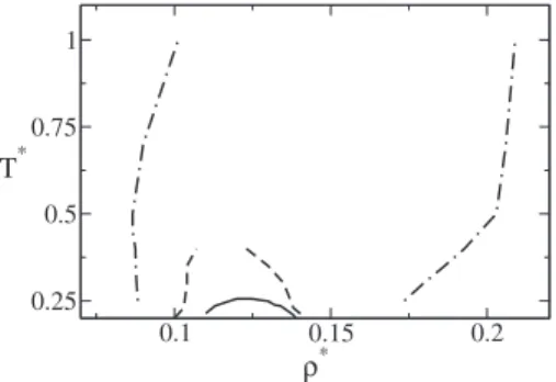
Figure1 illustrates the regions associated with the den-sity, diffusional, and structural anomalies of the model fluid studied here in the density-temperature planes. The region of density anomaly corresponds to state points for which
共/T兲P⬎0 and is bounded by the locus of points for which
the thermal expansion coefficient is zero. The translational diffusion coefficient as a function ofⴱ=3goes as follows. For the low temperature isotherms, the diffusivity increases
as the density is lowered, reaches a maximum atDmaxand
decreases until it reaches a minimum atDmin. The locus of
extrema in theD共兲curve mark the boundaries of the region
of diffusional anomaly, as shown in Fig. 1 using dashed
lines.
The region of structural anomaly of core-softened fluids is defined most simply using the translational or pair corre-lation order metric, defined as19
t⬅
冕
0c
兩g共兲− 1兩d, 共5兲
where ⬅r1/3 is the interparticle separation scaled by the mean interparticle distance, g共兲 is the radial distribution function andcis a scaled cutoff distance. In this work, we
use c=1
/3L/2, where L=V1/3. For a completely
uncorre-lated system共ideal gas兲g= 1 andtvanishes. In a crystal, the presence of long-range translational 共g⫽1兲 implies that t
depends on choice ofc. In simple liquids, tincreases with
isothermal compression. In liquids with waterlike anomalies
at low temperatures,tshows a nonmonotonic behavior. At a
given temperatureT, a structurally anomalous regime can be defined between densities t−max共T兲 and t−min共T兲 corre-sponding to locations of the maxima and minima in the translational order. In this structurally anomalous regime, shown using dot-dashed lines in Fig.1, an increase in density induces a decrease in translational order. The nested struc-tures of the anomalous regions is evident with the structur-ally anomalous regime enclosing the diffusion anomalous re-gion which in turn encloses the rere-gion of density anomaly.
III. INM ANALYSIS
In this section, we define the INM spectrum and explore how it can be used to connect the energy landscape of a liquid with its thermodynamic entropy. The potential energy of configurationrnearr0 can be written as a Taylor expan-sion of the form
U共r兲=U共r0兲−F•z+1
2r
T
•H•z 共6兲
where zi=
冑
mi共ri−r0兲 are the mass-scaled position coordi-nates of a particlei. The first and second derivatives ofU共r兲with respect to the vector z are the force and the Hessian
matrix, denoted byFandHrespectively. The eigenvalues of the HessianHare共兵i2其,i= 1 , 3N兲representing the squares of
normal mode frequencies, and W共r兲 are the corresponding
eigenvectors. In a stable solid,r0 can be conveniently taken
as the global minimum of the PESU共R兲, which implies that
F= 0 and Hhas only positive eigenvalues corresponding to
oscillatory modes. The INM approach for liquids interpretsr as the configuration at time trelative to the configurationr0 at timet0. Since typical configurations,r0 are extremely
un-likely to be local minima, therefore F⫽0 and H will have
negative eigenvalues. The negative eigenvalue modes are those which sample negative curvature regions of the PES, including barrier crossing modes. The ensemble-averaged INM spectrum,具f共兲典, is defined as
f共兲=
冓
1 3N兺
i=13N
␦共−i兲
冔
. 共7兲Quantities that are convenient for characterizing the INM
spectrum are 共i兲 the fraction of imaginary frequencies,
namely
Fim=
冕
imf共兲d, 共8兲
where the subscript in means that the integral is performed
only in the imaginary branch;共ii兲the fraction of real frequen-cies, that is
Fr=
冕
rf共兲d, 共9兲
where the subscriptrindicates that the integral is performed only in the real branch and 共ii兲the mean square or Einstein frequency,E, given by
E2=
冕
2f共兲d= 具TrH典
m共3N− 3兲, 共10兲
where the last equality comes from using Eq.共7兲and具TrH典 is the ensemble-averaged value of the trace of the Hessian.
The simplest approximation to the entropy that can be derived from the INM approach is to consider a liquid as a collection of 3Nsimple harmonic oscillators vibrating at the Einstein frequency. The entropy of a one-dimensional har-monic oscillator with frequencyis given by
s/kB= 1 − ln共ប兲. 共11兲
The entropy of an ideal gas of N particles in three dimen-sions will be given by
Sid NkB=
5
2− ln共⌳
3兲, 共12兲
where⌳=h/
冑
2mkBTis the thermal de Broglie wavelength. In three dimensions the entropy of the harmonic oscillators given by Eq.共11兲is multiplied by 3. The entropy per particle of the harmonic oscillator within Einstein approximationsbecomess
E. In this case, the excess entropy of the Einstein
model of the liquid is given by the subtraction of the ideal gas entropic contribution, Eq.共12兲, fromNs
E/kBto give
0.1 0.15 0.2
ρ∗ 0.25
0.5 0.75 1
T*
SexE/Nk
B=
1 2+
3 2ln
冉
2kBT2
/3
mE2
冊
, 共13兲whereEis given by Eq.共10兲. This expression for the excess
entropy forms the basis of quasiharmonic cell model ap-proaches to understand entropy scaling of transport proper-ties, which have had only limited success.27In this study, we compare the Einstein frequency-based expression for the ex-cess entropy with the pair correlation entropy to obtain a better microscopic insight into the differences.
An alternative approach is to consider the liquid to be composed on average of a set of 3NFr harmonic oscillators
and a set of 3NFim degrees of freedom associated with the imaginary or unstable modes. The total thermodynamic en-tropy of the liquid can be written as a sum of contributions from the real and imaginary branches,
S=Sr+Sim. 共14兲
Using Eq.共11兲,Srcan be obtained by integrating the real
branch of the INM distribution as follows:
Sr/kB= 3N
冕
rf共兲s共兲d, 共15兲
where f共兲 is the INM probability density at frequency
given by Eq.共7兲. Contribution of the imaginary modes to the entropy must then be
Sim=S−Sr=Sid+Sex−Sr. 共16兲
In the present work, we use the above equations to esti-mateSrandSim; the per particle values of these quantities in units of kB are labeled srⴱ and simⴱ . To our knowledge, this decomposition of the entropy has not been used previously.
A somewhat parallel approach was used by Goddardet al.63
to treat the entropy of a liquid as a sum of contributions from a harmonic component and a hard-sphere fluid component.
IV. RESULTS
A. Excess entropy and diffusivity
The excess entropy is defined as the difference between the entropy of the real fluid and that of the ideal gas at the same temperature and density. Figure2illustrates the density
dependence of the excess 共represented in the figure by
dashed lines兲and pair correlation entropy共represented in the
figure by solid lines兲for four different isotherms. The values of the thermodynamic excess entropy, sexⴱ, have been taken
from the work of Mittalet al.35
The sexⴱ共兲 curves at low temperatures show a
pro-nounced excess entropy anomaly, corresponding to a rise in excess entropy on isothermal compression. Such an entropy anomaly is characteristic of waterlike liquids18,32–34and con-trasts with the behavior of simple liquids where free volume arguments are sufficient to justify a monotonic decrease in
entropy on isothermal compression. Figure 2 also compares
sexⴱ共兲ands 2
ⴱ共兲curves at four temperatures. It is evident that
s2ⴱessentially captures the anomalous behavior present ins ex ⴱ.
The effect of the higher-order multiparticle correlations terms insexⴱ is to generate a downward shift in the values of
the entropy and to attenuate the entropy anomaly. In the case of simple liquids, the residual multiparticle entropy, ⌬sⴱ
=sexⴱ −s 2
ⴱ, is typically of the order of 10%–15% of s ex
ⴱ for a
fairly wide range of densities. Clearly in the case of the core-softened modeled fluids, the residual multiparticle en-tropy contribution is larger in magnitude and more strongly density dependent. The anomalous pair entropy regime at a given temperature is an interval of densities s2max⬍ ⬍s2min within which 共S2/兲T⬎0. This can be identified
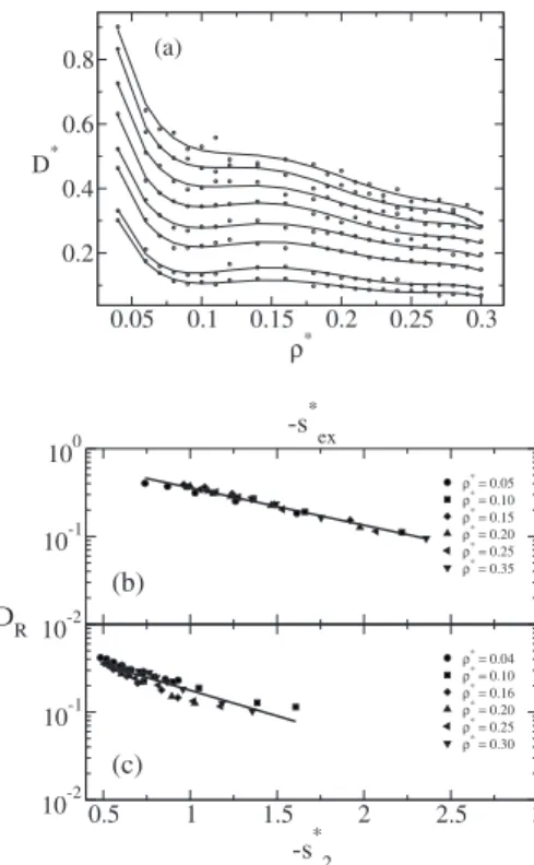
from the locus of extrema ins2共兲shown in Fig. 10. We now consider the scaling relationship between the diffusivity and the excess entropy. The diffusivity as a func-tion of density for different isotherms is shown in Fig. 3共a兲. Clear maxima and minima in theD共兲curves can be identi-fied at low temperatures. Figures 3共b兲 and 3共c兲 show the scaling of the reduced diffusivity, DR, with the excess, sexⴱ, and pair, s2ⴱ, entropy. Using the Rosenfeld macroscopic
re-0 0.1 0.2 0.3
ρ∗
-3 -2 -1 0
s*
FIG. 2. The pair correlation entropy,s2ⴱ共solid lines兲, and the excess entropy,
sexⴱ 共Ref. 35兲 共dashed lines兲 against density for fixed temperatures for
Tⴱ= 0.2, 0.3, 0.4, 0.5 from bottom to top.
0.05 0.1 0.15 0.2 0.25 0.3
ρ∗
0.2 0.4 0.6 0.8
D*
(a)
-s*
ex
10-2 10-1 100
D
R
ρ∗= 0.05 ρ∗= 0.10 ρ∗
= 0.15 ρ∗
= 0.20 ρ∗
= 0.25 ρ∗= 0.35
0.5 1 1.5 2 2.5 3
-s*
2
10-2 10-1
ρ∗
= 0.04 ρ∗= 0.10 ρ∗= 0.16 ρ∗= 0.20 ρ∗
= 0.25 ρ∗
= 0.30
(b)
(c)
FIG. 3. 共a兲 Diffusion vs reduced density for fixed temperatures Tⴱ = 0.2, 0.23, 0.30, 0.35, 0.40, 0.45, 0.50, 0.55 from bottom to top;共b兲diffusion in Rosenfeld units vs the negative of the −sexⴱ and共c兲diffusion in Rosenfeld
units as a function of −s2ⴱ.
duction parameters for the length as −1/3 and the thermal velocity as 共kBT/m兲1
/2, the dimensionless diffusivity is
de-fined as
DR⬅D
1/3
共kBT/m兲1
/2. 共17兲
The scaling of the reduced diffusivity,DR withsexⴱ is excel-lent withDR=AeBsex
ⴱ
whereA= 0.95 andB= 0.98. The scaling with the pair entropy,s2ⴱ, shows a weak isochore dependence
and the line of best fit is obtained with A= 0.68 and B
= 1.35. The comparison between the Figs.3共b兲 and3共c兲 in-dicates that for our anomalous fluid, the diffusivity scaling with the pair correlation entropy is not as universal as with the excess entropy. This is likely to be a consequence of the presence of two density-dependent length scales, in such wa-terlike fluids when compared to simple liquids, such as the Lennard-Jones fluid.
B. INM analysis
Next, we present the results from our INM analysis of the simulation for the core-softened fluid. The INM spectra along theⴱ= 0.11 isochore for various temperatures is
illus-trated in Fig. 4共a兲 while the INM spectra along the Tⴱ
= 0.20 isotherm for various densities is illustrated in Fig.
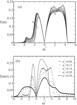
4共b兲. The shape of the INM spectra have the characteristic real and imaginary branches. As in the case of Lennard-Jones and Morse liquids,45,58the negative modes shrink in intensity and go to low frequencies as the temperature is decreased, while the peak of the real branch increases. Unlike in the case of simple liquids, however, both the real and the imagi-nary branch have a pronounced bimodality which can be clearly seen for the spectra along the ⴱ= 0.11 isochore.
which must be connected with two different length scales of the potential. Figure4共b兲shows that along theTⴱ= 0.20
iso-therm, the bimodality in the imaginary branch is most pro-nounced within the anomalous regime and is attenuated at both low and high densities. In contrast, the bimodality of the real branch persists even at high densities. It would be interesting to explore in future work if this bimodal fre-quency distribution results in multiple-time-scale behavior analogous to that seen in hydrogen-bonded liquids, such as water and methanol.51,64–66
The Einstein frequency is the second moment of the INM distribution, as defined in equation Eq.共10兲, and repre-sents an effective frequency describing the very short-time, local dynamics of the particles. Figure 5 illustrates the be-havior of Einstein frequency for the core-softened potential. For a fixed temperature, increasing density results in increase of Eⴱ=
冑
m2/⑀, indicating stronger trapping of the liquid particles in local cages. This is consistent with the behavior of simple liquids observed in earlier studies.45,58TheEⴱ
val-ues is virtually independent of temperature forⴱ⬇0.05 and
ⴱ⬇0.125. At low densities,
E
ⴱ shows a small decrease with
increasing temperature while at higher densities, there is a weak minimum in the Eⴱ at intermediate temperatures. The
density dependence ofEⴱ carries no significant signatures of
the diffusivity anomaly.
The fraction of imaginary modes, Fim, indicates how
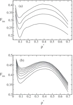
much the system samples regions with negative curvature which is known to be strongly correlated with the diffusivity.67 Figure6 shows density dependence fraction of
imaginary modes, Fim, for our core-softened anomalous
fluid. In simple liquids, Fim decreases with density and the graph Fim versus ⴱ always exhibit a negative slope.
45,58 In contrast, for the core-softened potential studied here, Fim shows very pronounced non-monotonic behavior For very low,⬍Fmin, and very high,⬎Fmax, densities,Fimhas a negative slope, decreasing with increasing density. For inter-mediate densities,Fmax⬎⬎Fmax,Fimincreases with den-sity. The density,Fⴱmin⬇0.1, is almost temperature
indepen-dent. The location of the maximum in Fim共兲 curve is
Fⴱmax⬇0.4 at low temperatures, but shifts to lower densities
with increasingTⴱ.
A comparison of the behavior of Fim共兲, illustrated in Fig.6, and D共兲, illustrated in Fig.3shows that the density
of minimumFimcoincides with the density of minimum D.
In contrast, the density of maximumFim occurs at densities much higher than the density of maximum diffusivity.
More--6 -4 -2 0 2 4 6
ω∗
0 0.05 0.1 0.15 0.2 0.25
f(ω)
(a)
-6 -4 -2 0 2 4 6 8 10
ω∗
0 0.05 0.1 0.15 0.2 0.25
f(ω)
ρ∗=0.06 ρ∗=0.12 ρ∗=0.14 ρ∗=0.20 ρ∗=0.30
(b)
FIG. 4.共a兲INM spectra as a function of frequency forTⴱ= 0.20, 0.23, 0.30, 0.35, 0.40, 0.45, 0.50, and 0.55 andⴱ= 0.11. The arrows indicate the in-crease of the temperature.共b兲INM spectra as a function of frequency for Tⴱ= 0.20 andⴱ= 0.06, 0.12, 0.14, 0.20, 0.30.
0.05 0.1 0.15 0.2 0.25 0.3 ρ∗
2 3 4 5
ω∗Ε
T*= 0.20 0.30 0.40 0.50
4.6 4.7 4.8
ω∗ Ε
0.2 0.3 0.4 0.5 T* 1.9
2
ω∗Ε
ρ∗= 0.08 ρ∗
= 0.23
over, the region in whichFimshows an anomalous increase with compression persists to very high temperatures, well above the temperature for onset of structurally anomalous behavior. In order to understand this behavior, we compare the zeroth, first and second derivatives of the potential as a function of pair separation with Fimfor Tⴱ= 1.0 plotted as a
function of the mean interparticle separation,−1/3in Fig.7. It is immediately obvious that the location of the minimum
of Fim coincides with the location of the minimum of the
second derivative. For densities lower than this minimum, the second derivative increases and the number of imaginary modes decreases. Clearly, this effect persists in the high-temperature fluid where binary collisions dominate the dy-namics since it reflects the curvature of the pair interaction.
V. INM SPECTRA AND LIQUID-STATE ENTROPY
In Sec. III, we discuss the possibility of partitioning the entropy of a liquid into contributions,Sr andSim, associated with real and imaginary branches respectively of the INM
spectrum. The Sr contribution is directly derived from the
frequency distribution of the real branch while the Sim con-tribution is given bySim=S−Sr. In order to get a better
un-derstanding of the role played by each contribution to the
entropy, Fig. 8 shows the behavior with density for a fixed
temperature ofsimⴱ ,s
r
ⴱ,s id ⴱ, ands
ex
ⴱ. It is immediately evident
that srⴱshows a very similar density dependence tos id ⴱ, even
though the numerical value ofsrⴱis significantly lower. Other
than a small inflection atⴱ⬇0.1, the contribution of the real
INM modes to the entropy carries virtually no signature of the structural, entropy or diffusivity anomalies. The non-monotonic behavior ofsexⴱ in the anomalous regime seems to
be reflected only insimⴱ . The strong resemblance betweens id ⴱ
andsrⴱinT-and-dependence suggests that this term reflects
the generic effects of thermal fluctuations and spatial con-finement on the entropy but in general it is insensitive to the structural details associated with the interplay between the two length scales in the anomalous regime.
Figure 9 compares, for various isotherms, the density
dependence of three different entropy estimators:共a兲simⴱ , the
imaginary mode contribution to the entropy, 共in the graph, form the value of simⴱ it is subtracted 2兲, 共b兲 s
2
ⴱ, the pair
correlation entropy, and共c兲s E
ⴱ , the entropy estimated using
the Einstein model for the liquid, Eq.共13兲. As discussed in Sec. IV A, the s2ⴱ behavior is very similar in density and
temperature dependence tosexⴱ, indicating that the pair
corre-lation contribution to the entropy is sufficient to capture the essential features of the anomalies. s
E
ⴱ , derived from the
Einstein model, is very similar tosrⴱ, presumably because of
0.1 0.2 0.3 0.4 0.5 0.6 0.7
ρ∗ 0.2
0.25 0.3 0.35 0.4
F
im
(a)
0 0.1 0.2 0.3 0.4 0.5 0.6 0.7
ρ∗ 0.3
0.35 0.4 0.45 0.5
F
im
(b)
FIG. 6. 共a兲 Fraction of imaginary modes against density for fixed temperatures Tⴱ= 0.20, 0.30, 0.40, 0.55 from bottom to top. 共b兲 Fraction of imaginary modes against density for fixed temperatures Tⴱ = 0.80, 1.0, 1.20, 1.40, 1.60.1.80, 2.0, 2.2 from bottom to top.
1 1.5 2 2.5 3
r/σ -5
0 5 10
U*(r)
-dU*/dr*
d2U*/dr*
2
Fi
FIG. 7. Potential, force, and second derivative of the potential in units of⑀
andFimⴱ15.0− 1.0 forTⴱ= 1.0 vs reduced distance.
0 0.1 0.2 0.3
ρ∗ -2
0 2 4
s* s*
r
s*
id
s*
im
s*
ex
FIG. 8. sidⴱ,srⴱ,simⴱ, andsexⴱ vs density forTⴱ= 0.2.
0 0.1 0.2 -6
-5 -4 -3 -2 -1 0
s
0 0.1 0.2 0 0.1 0.2
ρ∗
s2* s
im *
s* ωE
(a) (b) (c)
FIG. 9. 共a兲simⴱ − 2.0 obtained from Eq.共16兲withsimⴱ obtained from Ref.35,
共b兲s2ⴱand共c兲from the Einstein Frequency. See the text for more details.
In all cases, the entropy is plotted against density for fixed temperatures Tⴱ= 0.20, 0.30, 0.40 and 0.50 from bottom to top.
the use of the harmonic oscillator representation of the en-tropy. The nonmonotonic behavior ofE共兲 results in small
plateau at low temperatures. The overall decrease inSEwith
density is much too steep and monotonic compared withsexⴱ
ands2ⴱ. In contrast, s im ⴱ =sⴱ−s
r
ⴱ, captures the behavior of the
entropy within the anomalous region very successfully. The relative displacement ofsimⴱ 共兲curves for different isotherms
is very small, consistent with the earlier observation that the overall effect of thermal and free volume effects is better captured by srⴱ.
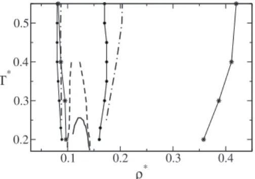
As a summary of the insights obtained from INM analy-sis and pair correlation entropy into the nested cascade of anomalies picture of waterlike liquids, we use the extrema in
Fim共兲 and s2ⴱ共兲 curves to define additional anomalous re-gimes within which 共Fim/兲T⬎0 and 共s2ⴱ/ⴱ兲T⬎0
re-spectively, as shown in Fig.10. The low density boundaries of anomalous regime in t, Fim, and s2ⴱ almost coincide,
re-flecting the onset of the steep repulsive wall. The
high-density boundary of the anomalous regime ofFimoccurs at
very high densities. In contrast, the high density limit of the anomalous regime ins2ⴱis very close to that defined byt, and
also bysimⴱ though the latter is not shown in the figure.
VI. CONCLUSIONS
This paper explores the connection between entropy, dif-fusivity and the PEL of a core-softened fluid with waterlike anomalies using MD simulations and INM analysis.
We demonstrate that the diffusivity and the excess en-tropy of a core-softened fluid with isotropic pair interactions obey Rosenfeld-type excess entropy scaling of transport properties. The use of macroscopic reduction parameters for the diffusivity based on temperature and density is particu-larly appropriate for fluids with multiple length scales where defining an effective hard-sphere radius is inappropriate. We also show that the substituting the excess entropy by the pair correlation entropy leads to a weak isochore dependence of the Rosenfeld-scaling parameters, not seen in simple liquids but observed in other waterlike liquids.68
The INM spectra, including the Einstein frequency and the fraction of imaginary modes, is computed over a wide range of temperatures and densities. INM analysis is shown
to provide unexpected insights into the dynamical conse-quences of the interplay between length scales characteristic of anomalous fluids that cannot be obtained from an equilib-rium transport property such as the diffusivity.
Both the real and imaginary branches of the INM spectra exhibit bimodality that has so far not been observed. As a function of density along an isotherm, the bimodality in the real branch of the INM spectrum persists to very high den-sities well beyond the structurally anomalous region. In con-trast, the bimodality of the imaginary branch is much more closely correlated with the region of the structural anomaly. The bimodal character of the both branches of the INM spec-trum suggests that such core-softened fluids may show mul-tiple time-scale behavior similar to that seen in hydrogen-bonded systems.
The Einstein frequency shows an essentially monotonic dependence on density along an isotherm. The temperature dependence of the Einstein frequency is weak and monotoni-cally decreasing with temperature at low densities and non-monotonic at high temperatures. In contrast to the Einstein frequency, the fraction of imaginary frequencies shows very anomalous behavior in comparison to simple liquids, with an
extended density regime over which Fim increases with
in-creasing density. While the low density boundary of this re-gion coincides with that of the structural anomaly, the high density boundary occurs at very high densities well beyond the structurally anomalous regime. Previous INM studies of liquids have largely connected the diffusivity with the frac-tion of imaginary modes. Our results show that informafrac-tion about diffusivity is largely contained in the behavior of the imaginary branch of the INM spectra, but factors such as the bimodality of the frequency distribution in this branch must be considered in addition toFim.
Given the validity of excess entropy scaling for the dif-fusivities, we introduce INM-based estimators of the entropy, to connect the energy landscape with liquid state thermody-namics and kinetics. The conceptually simplest INM-based estimator is to treat the liquid as a collection of 3D harmonic oscillators vibrating at a single frequency, corresponding to the Einstein frequency. The Einstein model entropy shows a very steep decrease with density along isotherms with a very weak signature of the onset of the structurally anomalous regime.
An alternative approach to developing an INM-based es-timator of the entropy that we have explored is to assume that the total entropy of the fluid can be written as a sum of contributions from 3NFrharmonic modes and 3NFim imagi-nary modes. The real branch of the INM spectrum can be used to estimate the harmonic contribution,srⴱ, exactly. The
entropy contribution of the imaginary branch, simⴱ , is then
given by the difference of the thermodynamic entropy,s, and the real branch contribution,srⴱ. The temperature and density
dependence ofsrⴱcarries virtually no signature of the
liquid-state anomalies, and seems to reflect only the generic effects of thermal fluctuations and spatial confinement on the en-tropy In contrast, simⴱ =sⴱ−s
r
ⴱ, captures the behavior of the
entropy within the anomalous region very successfully though the relative displacement of simⴱ 共兲 curves for
differ-ent isotherms is too small. The extrema insimⴱ define a region
0.1 0.2 0.3 0.4
ρ∗ 0.2
0.3 0.4 0.5
T*
FIG. 10. Cascade of waterlike anomalies in the density-temperature plane. The solid line limits the region of density anomaly, the dashed line illus-trates the region of diffusion anomaly and the dot-dashed line shows the region of structural anomaly. The filled circles represent the density of mini-mum and maximini-mums2and the stars represent the region of minimum and
of anomalous entropy behavior in the density-temperature plane that is almost identical as the region within which
共S2/兲T⬎0.
The overall and somewhat unexpected outcome of our INM analysis of a core-softened waterlike fluid is that the real and imaginary frequency branches show very different sensitivities to the dynamical consequences of the interplay between two length scales in the anomalous regime of the liquid. Moreover, the entropy contribution from the imagi-nary frequency modes of the INM spectrum reflects the anomalous behavior of the excess entropy and diffusivity characteristic of waterlike fluids, but the real frequency branch does not.
ACKNOWLEDGMENTS
This work is supported by the Indo-Brazil Cooperation
Program in Science and Technology of the CNPq 共Brazil兲
and DST共India兲.This work is also partially supported by the CNPq through the INCT-FCx. The authors would like to thank Murari Singh for help with preparing some of the fig-ures.
1
F. H. Stillinger and T. A. Weber,Phys. Rev. A 25, 978共1982兲.
2
P. G. Debenedetti and F. H. Stillinger,Nature共London兲 410, 259共2001兲.
3
D. J. Wales,Energy Landscapes: With Applications to Clusters, Biomol-ecules and Glasses共Cambridge University Press, Cambridge, 2003兲.
4
J.-P. Hansen and I. R. McDonald,Theory of Simple Liquids共Academic, London, 2002兲.
5
F. Sciortino, E. La Nave, and P. Tartaglia,Phys. Rev. Lett. 91, 155701
共2003兲.
6
I. Saika-Voivod, P. H. Poole, and F. Sciortino,Nature共London兲 412, 514
共2001兲.
7
G. Franzese, G. Malescio, A. Skibinsky, S. V. Buldyrev, and H. E. Stan-ley,Nature共London兲 409, 692共2001兲.
8
A. Scala, F. W. Starr, and E. La Nave, F. Sciortino, and H. E. Stanley, Nature共London兲 406, 6792共2000兲.
9
E. La Nave, A. Scala, F. W. Starr, H. E. Stanley, and F. Sciortino,Phys. Rev. Lett. 84, 4605共2000兲.
10
E. A. Jagla,Phys. Rev. E 58, 1478共1998兲.
11
H. M. Gibson and N. B. Wilding,Phys. Rev. E 73, 061507共2006兲.
12
L. Xu, P. Kumar, S. V. Buldyrev, S.-H. Chen, P. Poole, F. Sciortino, and H. E. Stanley,Proc. Natl. Acad. Sci. U.S.A. 102, 16558共2005兲.
13
A. Barros de Oliveira, M. C. Barbosa, and P. A. Netz,Physica A 386,
744共2007兲.
14
A. Barros de Oliveira, P. A. Netz, T. Colla, and M. C. Barbosa,J. Chem. Phys. 124, 084505共2006兲.
15
A. B. de Oliveira, P. A. Netz, T. Colla, and M. C. Barbosa,J. Chem. Phys. 125, 124503共2006兲.
16
D. Y. Fomin, D. Frenkel, N. V. Gribova, and V. N. Ryzhov,J. Chem. Phys. 129, 064512共2008兲.
17
S. A. Egorov,J. Chem. Phys. 128, 174503共2008兲.
18
J. Mittal, J. R. Errington, and T. M. Truskett,J. Chem. Phys.125, 076102
共2006兲.
19
J. R. Errington and P. G. Debenedetti,Nature共London兲 409, 318共2001兲.
20
P. A. Netz, F. W. Starr, H. E. Stanley, and M. C. Barbosa,J. Chem. Phys. 115, 344共2001兲.
21
P. A. Netz, F. W. Starr, M. C. Barbosa, and H. E. Stanley,J. Mol. Liq. 101, 159共2002兲.
22
S. Zhou,Phys. Rev. E 77, 041110共2008兲.
23
N. M. Barraz, E. Salcedo, and M. C. Barbosa, J. Chem. Phys. 131,
094504共2009兲.
24
P. Camp,Phys. Rev. E 68, 061506共2003兲.
25
Y. Rosenfeld,Phys. Rev. A 15, 2545共1977兲.
26
Y. Rosenfeld,Chem. Phys. Lett. 48, 467共1977兲.
27
Y. RosenfeldJ. Phys.: Condens. Matter 11, 5415共1999兲.
28
M. Dzugutov,Nature共London兲 381, 137共1996兲.
29
J. J. Hoyt, M. Asta, and B. Sadigh,Phys. Rev. Lett. 85, 594共2000兲.
30
A. Samanta, S. M. Ali, and S. K. Ghosh,Phys. Rev. Lett. 87, 245901
共2001兲.
31
A. Samanta, S. M. Ali, and S. K. Ghosh,J. Chem. Phys. 123, 084505
共2005兲.
32
R. Sharma, S. N. Chakraborty, and C. Chakravarty,J. Chem. Phys.125,
204501共2006兲.
33
M. Agarwal and C. Chakravarty,Phys. Rev. E 79, 030202共2009兲.
34
M. Agarwal, A. Ganguly, and C. Chakravarty, J. Chem. Phys. 113,
15284共2009兲.
35
J. R. Errington, T. M. Truskett, and J. Mittal,J. Chem. Phys.125, 244502
共2006兲.
36
T. Goel, C. N. Patra, T. Mukherjee, and C. Chakravarty,J. Chem. Phys. 129, 164904共2008兲.
37
H. S. Green,The Molecular Theory of Fluids共North-Holland, Amster-dam, 1952兲.
38
R. E. Nettleton and H. S. Green,J. Chem. Phys. 29, 1365共1958兲.
39
H. J. Raveché,J. Chem. Phys. 55, 2242共1971兲.
40
D. C. Wallace,J. Chem. Phys. 87, 2282共1987兲.
41
A. Baranyai and D. J. Evans,Phys. Rev. A 40, 3817共1989兲.
42
R. M. Stratt and M. Maroncelli,J. Phys. Chem. 100, 12981共1996兲.
43
R. M. Stratt,Acc. Chem. Res. 28, 201共1995兲.
44
T. Keyes,J. Phys. Chem. A 101, 2921共1997兲.
45
P. Shah and C. Chakravarty,J. Chem. Phys. 115, 8784共2001兲.
46
P. Shah and C. Chakravarty,J. Chem. Phys. 116, 10825共2002兲.
47
P. Shah and C. Chakravarty,Phys. Rev. Lett. 88, 255501共2002兲.
48
M. Cho, G. R. Fleming, S. Saito, I. Ohmine, and R. M. Stratt,J. Chem. Phys. 100, 6672共1994兲.
49
M. C. C. Ribeiro and P. A. Madden,J. Chem. Phys. 106, 8616共1997兲.
50
W.-X. Li, T. Keyes, and F. Sciortino,J. Chem. Phys. 108, 252共1998兲.
51
A. Mudi, C. Chakravarty, and R. Ramaswamy, J. Chem. Phys. 122,
104507共2005兲.
52
H. Thurn and J. Ruska,J. Non-Cryst. Solids 22, 331共1976兲.
53
Periodic table of the elements,http://periodic.lanl.gov/default.htm, 2007.
54
G. E. Sauer and L. B. Borst,Science 158, 1567共1967兲.
55
S. J. Kennedy and J. C. Wheeler,J. Chem. Phys. 78, 1523共1983兲.
56
T. Tsuchiya,J. Phys. Soc. Jpn. 60, 227共1991兲.
57
C. A. Angell, R. D. Bressel, M. Hemmatti, E. J. Sare, and J. C. Tucker,
Phys. Chem. Chem. Phys. 2, 1559共2000兲.
58
M. S. Shell, P. G. Debenedetti, and A. Z. Panagiotopoulos,Phys. Rev. E 66, 011202共2002兲.
59
P. H. Poole, M. Hemmati, and C. A. Angell,Phys. Rev. Lett. 79, 2281
共1997兲.
60
H. Tanaka,Phys. Rev. B 66, 064202共2002兲.
61
M. Agarwal, R. Sharma, and C. Chakravarty, J. Chem. Phys. 127,
164502共2007兲.
62
M. Agarwal and C. Chakravarty,J. Phys. Chem. B 111, 13294共2007兲.
63
S.-T. Lin, M. Blanco, and W. A. Goddard,J. Chem. Phys. 119, 11792
共2003兲.
64
A. Mudi, C. Chakravarty, and R. Ramaswamy, J. Chem. Phys. 124,
069902E共2006兲.
65
R. Sharma, C. Chakravarty, and E. Milotti,J. Phys. Chem. B 112, 9071
共2008兲.
66
M. Agarwal, H. R. Kushwaha, and C. Chakravarty, J. Phys. Chem. B 114, 651共2010兲.
67
G. Seeley and T. Keyes,J. Chem. Phys. 91, 5581共1989兲.
68
M. Agarwal, M. Singh, R. Sharma, M. P. Alam, and C. Chakravarty,J. Chem. Phys. B 114, 6995共2010兲; arXiv:1004.3091.