Note
Spatial variability of physical and chemical attributes of some
forest soils in southeastern of Brazil
Clayton Alcarde Alvares
1, José Leonardo de Moraes Gonçalves
2*, Sidney Rosa Vieira
3, Cláudio
Roberto da Silva
4, Walmir Franciscatte
51Instituto de Pesquisas e Estudos Florestais, Av. Comendador Pedro Morgante, 3500 – 13415-000 - Piracicaba, SP - Brasil. 2USP/ESALQ – Depto. de Ciências Florestais, C.P. 09 – 13418-900 – Piracicaba, SP – Brasil.
3IAC/Centro de Solos e Recursos Ambientais, Av. Barão de Itapura, 1481 – 13020-902 – Campinas, SP – Brasil. 4Fibria Celulose SA, Rod. General Euryale de Jesus Zerbini, km 84, SP 66 – 12300-000 – Jacareí, SP – Brasil. 5Fibria Celulose SA, Rod. Raul Venturelli, km 210, C.P. 28 – 18300-970 – Capão Bonito, SP – Brasil.
*Corresponding author <jlmgonca@usp.br> Edited by: Jussara Borges Regitano
ABSTRACT: Capão Bonito forest soils, São Paulo state, Brazil, have been used for forestry purposes for almost one century. Detailed knowledge about the distribution of soil attributes over the landscape is of fundamental importance for proper management of natural resources. The purpose of this study was to identify the variability and spatial dependence of chemical and physical attributes of Capão Bonito forest soils. A large soil database of regional land was raised and organized. Most of the selected variables were close to the lognormal frequency range. Soil texture presented a higher range in the A horizon, and the nugget effect and sill were greater in the B horizon. These differences are attributed to the parent material of the region (Itararé Geologic Formation), which presents uneven distribution of sediments. Chemical attributes related to soil fertility presented a higher spatial dependence range in the B horizon, probably as a result of more intensive management and erosion history of the superficial soil layer. Maps for some attributes were interpolated. These had specific areas of occurrence and a wide distribution along the perimeter of the Capão Bonito District Forest, allowing a future site-specific soil management.
Keywords: geostatistics, semivariogram, geographic information system, soil management, forestry precision
Introduction
Forest soil refers to a soil that has been developed by and/ or sustains some forest vegetation (Gonçalves, 2002). Capão Bonito forest soils, São Paulo state, Brazil, have been used for forestry purposes for almost one century. Pedologic survey his-tory from this region presents three phases: (i) soil map from the São Paulo state (SNPA, 1960), (ii) pedologic map from the São Paulo state (Oliveira, et al., 1999), (iii) semi-detailed pedologic surveys (Gonçalves, 1997; Rizzo, 2001). This evolution aimed to achieve a greater level of detail, but actually its interpretation is what allows a precise identification of forest management units (Gonçalves, 1988). The method used nowadays for soil cartographic representation is characterized by abrupt boundar-ies of mapping units. It is crucial to consider the spatial range of soil properties verifying other ways to represent them and providing a better final quality on generated maps (Burrough, 1991; Webster, 2008). Soil attributes must be considered as re-gional variables (Matheron, 1963) as numeric spatial functions that vary from one region to another with apparent extension whose variability cannot be represented by a simple mathematic function (Guerra, 1988).
Geostatistics has been widely applied in studies on forest soil variability. Several areas of forestry and ecology used the semivariogram as a tool to detect and understand the physical and chemical soil variability related to forest productivity (Bog-nola et al., 2008), the soil survey (Novaes Filho et al., 2007), and the forest management effects on soil (Lima et al., 2008).
These studies fulfilled a great demand for mapped information of edapho-pedologic attributes, mainly applying to agricultural productivity modeling, fertilization management and delimita-tion of management units. Therefore, geostatistic results should be used as a routine method to allow more precise recommen-dations (Vieira, 2000) for in-site soil management (Molin, 2001). This study was carried out with the aim of characterizing the variability and spatial dependence of chemical and physical at-tributes of Capão Bonito forest soils.
Materials and Methods
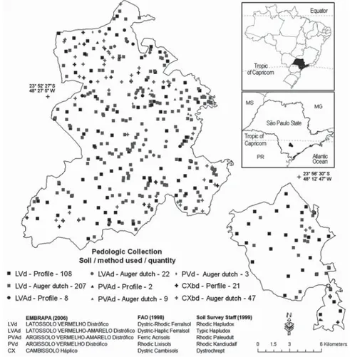
One hundred and eighty-three soil points sampled by Gonçalves (1997) and Rizzo (2001) were used, including 139 pedologic profiles and 44 samples collected with a Dutch auger. These data were obtained from printed reports, georeferenced and compiled in a soil database for the studied area. From 2006 to 2008, 244 more georeferenced samples collected with a Dutch auger were performed for all the planted areas aiming to review the pedologic mapping, in addition to increasing soil sampling, leading to a total of 427 soil point samples (Figure 1). The soil database from the Capão Bonito forest district includes local-ization information of each sample, soil and pedologic horizon type, horizon depth, sampling method and physical and chemical soil attribute values. All points are located in forest stand areas (21,883 ha). Among the sampling years 1997 and 2008 only a small percentage of this area suffered intervention of tillage. The techniques of tillage followed the precepts of the minimum soil preparation (Gonçalves et al., 2004). Soil samples have the same distribution of classes of pedological surveys. The soil types Rhodic Haplodux, Typic Hapodlux, Rhodic Paleudult, Rhodic Kandiudalf and Dystrochrept present, respectively, 82.5 %, 5.3 %, 1.4 %, 0.4 % and 10.4 % occurrence of pedological surveys (Gonçalves, 1997; Rizzo, 2001).
Data were grouped into files with three XYZ-type columns. XY values represented longitude and latitude of the sample (profile or Dutch auger) collected in the field, respectively, and
Z values represented pedological attributes of very fine sand (0.05 - < 0.1 mm), fine sand (0.1 - < 0.25 mm), medium sand (0.25 - < 0.5 mm), coarse sand (0.5 - < 1 mm), very coarse sand (1 - < 2 mm), total sand, silt (0.002 - < 0.05 mm), clay (< 0.002), silt/clay ratio, natural clay, soil organic matter (SOM), available phosphorus, exchangeable potassium, exchangeable calcium, exchangeable magnesium, exchangeable sodium, exchangeable aluminum, exchangeable aluminum + hydrogen, pH H2O, pH KCl, delta pH, sum of bases, effective CEC (cation exchange capac-ity) and CEC pH 7. Soil properties were evaluated out in the A and B horizons.
Exploratory data analysis was performed by the statistical program SYSTAT v.11 (Wilkinson, 2004). The exploratory step is crucial because it provides identification of possible diverse values and shapes of variable distribution. Position (mean, median and mode), dispersion (minimum, maximum and stan-dard deviation) and distribution measurements (coefficients of variation, skewness and kurtosis) were performed. Normality hypothesis was verified according to the W test at 5 % (Shapiro and Wilk, 1965) in which normal or logarithmic distribution tendencies were verified.
Experimental omnidirectional semivariograms were adjusted by the geostatistic program GS+ v.9. In this program, theoreti-cal model selection (semivariogram) is performed based on the smallest reduced sum of squares (RSS) and on the greatest
termination coefficient (R2) (Robertson, 2008). In some cases,
semivariograms were manually adjusted or “at feeling”, originat-ing more realistic and satisfactory results in relation to automatic adjustment by the GS+ v.9 program.
Experimental semivariograms were determined until approxi-mately 50 % of the geometric camp (Figure 1), since after this val-ue the semivariogram did not seem to be correct (Gval-uerra, 1988), i.e., its accuracy was reduced due to the small number of possible pairs to calculate the semivariance at this distance. A geometric camp of 12,000 m with partition groups (lags) of 1,200 m was considered, as these lags are the estimators of the experimental semivariograms (Deutsch and Journel, 1998). Although the study area is divided into two subareas, it was considered as one area, because it presents a small separation distance, and the subareas have the same topography and soil groups. Theoretical models considered, such as spherical, exponential, Gaussian and linear, were described by Guerra (1988), Vieira (2000) and Andriotti (2003). Only this theoretical semivariogram group was considered because it usually covers the general dispersion situation of soil science spatial events (Burrough and McDonnell, 1998; Soares, 2006). Through GS + v.9 cross validation, the correlation coef-ficient of selected models was obtained.
Scaled experimental semivariograms were calculated accord-ing to Vieira et al. (1997) by dividaccord-ing their values by data vari-ances, obtaining semivariograms with a sill close to 1.0. It was possible to plot many soil attributes on one graph along with their proximity when elected, indicating a similarity of range along landscapes (Vieira et al., 1997). The spatial dependence index (SDI) was used according to Zimback (2001), which mea-sures a sample’s structural variance effect on the total variance (sill). SDI comprises the following interpretation break: weak SDI ≤ 25 %, moderate SDI between 25 % and 75 % and strong SDI ≥ 75 %. This index is a complement of the traditional method recommended by Cambardella et al. (1994) in which the nugget weight effect (randomness) on total variance is evalu-ated. Through structural parameters obtained from experimental semivariograms, maps of some properties were created with the geographic information system ArcMap v.9.3 (ESRI, 2008). A punctual ordinary kriging estimator was used for geostatistic interpolation. To assist map interpretation, subtitles were com-posed with similar amounts by dividing the distribution into four groups that enclose the same occurrence area. Thus, each subtitle group represents 25 % of the mapped area.
Results and Discussion
Capão Bonito forest soils presented distinct textures (Table 1). Samples of the A horizon had 70 to 870 g kg–1
of total sand. Medium, coarse and very coarse sand presence was small (< 20 g kg–1
); few areas reached values of 441 g kg–1
(coarse sand in the A horizon). This feature became evident by high coefficients of skewness, low coefficient of kurtosis (platykurtic) and by closer tendency to a lognormal distribu-tion of medium, coarse and very coarse sand. Total, very fine and fine sand presented distributions close to normal, positive skewness and low kurtosis coefficient (leptokurtic). Oxidic soils from Capão Bonito presented an average of 115 g kg–1
of silt in the A horizon with positive skewness and platykurtic
distribution tending to be lognormal. The mean clay content in the B horizon (310 g kg–1
) was slightly more than that of the A horizon (284 g kg–1) due to the presence of the Rhodic
Kandiudalf in the area. Rhodic Hapludox with clayey texture was predominant, thus demonstrating a slight positive skew-ness for clay content; leptokurtic distribution was more similar to the lognormal. Similar results were obtained with the silt/ clay ratio with a mean value equal to 0.4. This ratio presented positive skewness and platykurtic distribution and was similar to the lognormal. The mean content of natural clay was 113 and 106 g kg–1 in the A and B horizons, respectively, presenting
positive skewness and a tendency to a lognormal distribution. Thus, these data clearly represent areas with a predominance of a Hapludox in which low clay dispersion and mobility are usual (EMBRAPA, 2006).
SOM presented a mean content of 23.5 g kg–1 in the A
ho-rizon and 13 g kg–1
in the B horizon (Table 1). SOM tended to the normal distribution and reduced positive skewness. Available phosphorus presented high skewness and kurtosis coefficients with mean contents of 4.4 and 3 mg kg–1
in the A and B hori-zons, respectively. Potassium, calcium and magnesium presented strong positive skewness, high kurtosis coefficients (platykurtic) and distributions tending to be lognormal. Mean values of potassium (0.7 mmolc kg
–1
), calcium (2.3 mmolc kg –1
) and mag-nesium (2 mmolc kg
–1
) in the A horizon were lower than the soil critical point (Gonçalves, 1995). The mean sodium content was 0.2 mmolc kg
–1
with strong skewness distribution to the left because most of the soils are poor in this element. Aluminum + hydrogen followed distributions tending to normal. Data of pH H2O and pH KCl in the A horizon presented a mean value
of 3.8 with distributions tending to normal. In the B horizon, the mean was 3.9 and the distribution tended to be lognormal. The maximum pH value recorded was 5.0 (pH H2O) and the minimum value was 2.6 (pH KCl). Delta pH values presented negative skewness and distribution close to normal. The most weathered soils were found at areas with delta pH values equal to 0.3 (positive balance charge).
The sum of bases presented high positive skewness and platykurtic distribution (high C.V.) tending to be lognormal. The mean of this attribute was very low, only 5.1 and 3 mmolc kg
–1
in the A and B horizons, respectively. The mean values of CEC were 24.7 mmolc kg
–1
(effective) and 85.7 mmolc kg –1
(pH7) for the A horizon. Their distributions presented negative positive skewness behavior only for CEC pH7 at the superficial layer. Most of the attributes, in both soil layers, presented distribu-tions tending to be lognormal. In other studies, this was also the best adjustment for most of the edaphic properties ( Cam-bardella et al., 1994; Zimback, 2001). The variables that required transformation, and with p-value close to zero by the normality test (Shapiro and Wilk, 1965), are presented in Table 1.
Table 1 – Results of descriptive exploratory analyses for soil attributes at 0 – 30 cm depth (A horizon) and at 30 – 80 cm depth (B horizon).
Measure of Kind of
Position Dispersion Distribution Distribution
Attribute Horizon Mean Median Mode Min8 Max9 S.D.10 C.V.11 S.C.12 K.C.13 Tendency (p-value)
Very fine sand1 A 70 74 70 0 170 37.8 51.1 0.7 0.2 ~ N14 0.0001
(g kg–1) B 70 79 60 10 220 38.7 48.8 0.9 1.3 ~ L15 0.0001
Fine sand1 A 370 379 300 30 747 179.0 47.2 0.1 -0.8 ~ N 0.0020
(g kg–1) B 360 367 290 10 739 183.9 50.2 0.1 -0.8 ~ N 0.0060
Medium sand1 A 70 90 30 10 320 68.1 75.6 1.1 0.7 ~ L 0.0001
(g kg–1) B 50 74 20 10 340 62.8 84.9 1.4 2.2 ~ L 0.0001
Coarse sand1 A 20 47 10 0 441 74.5 157.1 3.1 10.3 ~ L 0.0001
(g kg–1) B 20 47 10 0 418 70.4 150.7 2.8 9.5 ~ L 0.0001
Very coarse sand1 A 0 3 0 0 60 7.0 285.1 5.3 37.7 ~ L 0.0001
(g kg–1) B 0 3 0 0 40 7.0 230.0 3.3 12.8 ~ L 0.0001
Total sand A 567 540 730 70 870 189.3 35.0 -0.5 -0.7 ~ N 0.0001
(g kg–1) B 540 522 410 40 850 188.4 36.1 -0.4 -0.6 ~ N 0.0001
Silt1 A 116 139 100 10 556 83.8 60.1 1.7 4.0 ~ L 0.0001
(g kg–1) B 120 141 100 10 555 86.1 61.2 1.8 4.6 ~ L 0.0001
Clay1 A 284 320 160 99 840 164.4 51.4 0.8 0.0 ~ L 0.0001
(g kg–1) B 310 338 340 62 860 168.5 49.9 0.8 0.1 ~ L 0.0001
Silt/clay ratio A 0.4 0.5 0.3 0.1 2.3 0.4 71.7 1.4 1.9 ~ L 0.0001
B 0.4 0.5 0.3 0.0 3.6 0.4 80.7 2.5 11.9 L17 0.0001
Natural clay A 113 130 40 20 1000 190.5 1.5 3.8 14.7 ~ L 0.0001
(g kg–1) B 106 107 20 20 1000 190.5 1.8 4 16 ~ L 0.0001
Soil organic matter2 A 23.5 24.7 23.0 1.0 56.0 10.3 41.7 0.5 0.3 ~ N 0.0020
(g kg–1) B 13.0 14.9 10.0 0.5 36.0 8.5 56.1 0.6 -0.4 ~ N 0.0001
Phosphorus3 A 4.4 6.0 4.0 1.0 51.3 6.1 103.0 5.0 28.0 ~ L 0.0001
(mg kg–1) B 3.0 2.9 3.0 0.0 18.0 1.8 58.9 3.6 28.1 ~ L 0.0001
Exchangeable potassium3 A 0.7 1.2 0.5 0.1 15.3 1.8 147.5 5.5 36.3 ~ L 0.0001
(mmolc kg–1) B 0.4 0.7 0.2 0.1 11.4 1.1 153.3 6.1 49.2 ~ L 0.0001
Exchangeable calcium4 A 2.3 5.1 1.0 0.5 49.0 7.5 148.2 3.3 12.2 ~ L 0.0001
(mmolc kg–1) B 1.0 1.9 1.0 0.6 13.0 1.7 90.8 3.6 15.9 ~ L 0.0001
Exchangeable magnesium4 A 2.0 2.9 1.0 0.3 25.0 3.2 108.5 3.2 14.4 ~ L 0.0001
(mmolc kg–1) B 1.0 1.4 1.0 0.0 14.0 1.5 111.1 5.1 34.2 ~ L 0.0001
Exchangeable sodium3 A 0.2 0.8 0.2 0.0 29.0 3.5 440.2 7.6 57.6 ~ L 0.0001
(mmolc kg–1) B 0.2 0.6 0.2 0.0 20.0 2.8 409.7 6.3 38.7 ~ L 0.0001
Exchangeable aluminum4 A 17.0 17.4 18.0 0.0 55.0 9.0 52.0 0.6 1.1 ~ N 0.0001
(mmolc kg–1) B 14.8 14.5 15.0 0.0 41.0 6.4 43.9 0.5 1.5 ~ N 0.0030
Exchangeable aluminum +
hydrogen5 A 78.1 74.8 90.0 7.3 182.0 26.5 35.4 -0.1 1.0 ~ N 0.0020
(mmolc kg–1) B 51.2 51.3 40.0 2.9 109.0 21.2 41.3 0.0 -0.2 N16 0.5980
pH H2O6 A 3.8 3.9 3.6 3.4 5.0 0.4 10.0 0.9 0.1 ~ N 0.0001
B 3.9 3.9 3.8 3.4 4.6 0.2 6.3 0.5 0.2 ~ L 0.0001
pH KCl7 A 3.8 3.9 3.7 2.6 4.8 0.3 7.7 0.0 1.7 ~ N 0.0001
B 3.9 3.9 3.9 3.5 4.9 0.2 4.5 1.8 8.2 ~ L 0.0001
Delta pH A 0.0 -0.1 0.0 -1.1 0.3 0.3 -198.4 -1.2 0.7 ~ N 0.0001
B 0.0 0.0 0.0 -0.9 0.4 0.2 -543.4 -0.9 2.3 ~ N 0.0001
Sum of bases A 5.1 9.5 2.6 1.4 71.4 11.2 117.9 2.9 9.5 ~ L 0.0001
(mmolc kg–1) B 3.0 4.5 2.4 0.8 25.7 4.2 92.9 3.1 9.7 ~ L 0.0001
Effective CEC A 24.7 27.5 29.2 4.4 80.5 12.2 44.5 1.3 2.3 ~ L 0.0001
(mmolc kg–1) B 18.4 19.6 17.6 2.7 58.2 8.1 41.6 1.5 4.2 ~ N 0.0001
CEC pH7 A 85.7 84.6 74.2 2.9 189.1 28.7 33.9 -0.1 0.8 ~ N 0.0300
(mmolc kg–1) B 56.6 56.4 57.6 12.5 115.0 20.6 36.6 0.1 -0.1 N 0.5900
Methods (EMBRAPA, 1999): 1 = Densimeter; 2 = Walkley-Black; 3 = Mehlich 1; 4 = KCl 1 mol L–1; potential acidity (5 = calcium acetate 1
mol L–1); Active acidity (6 = H
2O deionized; 7 = KCl 1 mol L
–1); 8Min = minimum value observed; 9Max = maximum observed value; 10S.D.
= Standard Deviation; 11C.V. = Coeffi cient of variation; 12S.C. = skewness coeffi cient; 13K.C. = Kurtosis coeffi cient; 14~ N = Distribution
at this sampling intensity. This indicated that the sampling intensity was insufficient to detect the spatial dependence of these variables, considering the scale of a usual semi-detailed pedologic survey.
Very fine sand, medium sand, coarse sand, total sand, silt, clay and natural clay content in the A horizon were adjusted
to exponential functions, whereas very fine sand, total sand, silt and clay content were adjusted to spherical models. Other texture variables, such as fine sand, very coarse sand and silt/ clay ratio in both soil layers were also modeled with exponential functions. Both theoretical semivariogram models presented a rapid rise at the origin in which a linear behavior could be seen
Table 2 – Models, parameters and quality of experimental semivariograms adjusted to Capão Bonito forest soil data base in the 0 - 30 cm layer (A horizon) and 30 - 80 cm layer (B horizon).
Attribute Horizon Model Co5
Co + C6
Ao7
C/(Co + C) S.D.I.8 9
R2
S.S.R.10 11
r
Very fine sand A Exp.1 651 1508 3,840 57 moderate 0.55 1.44 105 0.21
(g kg–1) B Sph. 1 0.07 0.28 2,650 74 moderate 0.62 5.92.10–3 0.45
Fine sand A Exp. 9,550 33,550 10,320 72 moderate 0.98 5.84.106 0.64
(g kg–1) B Exp. 16,210 37,760 19,440 57 moderate 0.97 6.65.106 0.57
Medium sand A Exp. 0.49 0.98 20,370 50 moderate 0.75 3.69.10–1 0.33
(g kg–1) B Gau.3 0.69 1.37 22,308 50 moderate 0.84 2.68.10–2 0.04
Coarse sand A Exp. 1.65 2.63 5,857 37 moderate 0.61 2.60.10–1 0.18
(g kg–1) B Lin.4 1.17 1.17 11,411 0 weak 0.06 1.15.10–1 0.03
Very coarse sand A Exp. 0.47 0.94 8,970 50 moderate 0.74 3.53.10–2 0.28
(g kg–1) B Exp. 0.63 0.98 8,476 36 moderate 0.81 1.42.10–2 0.30
Total sand A Exp. 14,500 43,220 15,480 66 moderate 0.95 2.73.107 0.65
(g kg–1) B Sph. 16,552 37,470 10,330 56 moderate 0.95 2.14.107 0.57
Silt A Exp. 0.28 0.36 11,282 23 weak 0.76 1.54.10–3 0.30
(g kg–1) B Sph. 0.31 0.37 8,612 15 weak 0.32 2.72.10–3 0.22
Clay A Exp. 0.10 0.33 16,900 68 moderate 0.95 1.44.10–3 0.70
(g kg–1) B Sph. 0.12 0.27 10,928 56 moderate 0.93 1.56.10–3 0.64
Silt/clay ratio A Exp. 0.29 0.46 6,151 38 moderate 0.78 4.11.10–3 0.36
B Exp. 0.37 0.53 7,003 30 moderate 0.57 9.71.10–3 0.30
Natural clay A Exp. 0.001 1.25 3,300 100 strong 0.85 5.00.10–2 0.21
(g kg–1) B Lin. 1.00 1.00 11,394 0 weak 0.00 9.76.10–2 0.09
Soil organic matter A Gau. 0.22 0.28 4,954 20 weak 0.68 1.33.10–3 0.24
(g kg–1) B Exp. 41 84 12,720 51 moderate 0.89 1.27.102 0.38
Phosphorus-resin A Gau. 0.26 0.33 5,855 22 weak 0.81 1.72.10–3 0.13
(mg kg–1) B Lin. 0.31 0.31 11,389 0 weak 0.00 1.70.10–2 0.15
Exchangeable potassium A Exp. 0.37 0.63 2,874 41 moderate 0.70 5.06.10–3 0.18
(mmolc kg–1) B Gau. 0.43 0.83 6,581 48 moderate 0.90 1.96.10–2 0.95
Exchangeable calcium A Sph. 0.67 0.92 8,880 27 moderate 0.94 4.57.10–3 0.28
(mmolc kg–1) B Exp. 0.21 0.48 22,290 56 moderate 0.91 3.33.10–3 0.28
Exchangeable magnesium A Exp. 0.40 0.69 5,324 42 moderate 0.93 2.60.10–3 0.34
(mmolc kg–1) B Sph. 0.26 0.45 5,680 44 moderate 0.77 1.01.10–2 0.00
Exchangeable sodium A Lin. 0.50 0.50 11,391 0 weak 0.00 2.80.10–1 0.14
(mmolc kg–1) B Lin. 0.42 0.42 11,389 0 weak 0.00 4.84.10–1 0.15
Exchangeable aluminum A Gau. 64 99 16,603 35 moderate 0.83 2.08.102 0.25
(mmolc kg–1) B Lin. 34 37 11,389 9 weak 0.29 2.14.101 0.04
Exchangeable
aluminum+hydrogen A Exp. 367 756 5,110 52 moderate 0.56 3.39.10
4 0.41
(mmolc kg–1) B Exp. 268 465 5,415 42 moderate 0.44 1.64.104 0.40
pH H2O A Exp. 0.08 0.20 13,440 61 moderate 0.96 2.99.10–4 0.42
B Exp. 0.04 0.06 3,788 39 moderate 0.43 1.44.10–4 0.29
pH KCl A Sph. 0.05 0.19 15,820 72 moderate 0.93 1.91.10–4 0.42
B Lin. 0.03 0.03 11,388 0 weak 0.46 7.39.10–5 0.04
Delta pH A Exp. 0.02 0.09 5,490 79 strong 0.73 6.56.10–4 0.35
B Sph. 0.02 0.05 3,730 66 moderate 0.87 5.66.10–5 0.34
Sum of bases A Sph. 0.46 0.66 1,460 29 moderate 0.97 1.66.10–3 0.35
(mmolc kg–1) B Exp. 0.16 0.36 6,405 56 moderate 0.65 8.02.10–3 0.25
Effective CEC A Exp. 0.09 0.20 6,349 57 moderate 0.84 1.57.10–3 0.44
(mmolc kg–1) B Lin. 53 53 11,388 0 weak 0.27 1.52.102 0.12
CEC pH7 A Exp. 461 965 6,564 52 moderate 0.81 3.12.104 0.45
(mmolc kg–1) B Gau. 343 499 9,982 31 moderate 0.31 1.40.104 0.36
1Exp = exponential; 2Sph = spherical; 3Gau = gaussian; 4Lin = linear; 5Co = nugget; 6Co+C = Sill (C = structural variance); 7Ao = range
(meters); 8S.D.I. = spatial dependence index, 9R2 = model adjustment determination coeffi cient; 10R.S.S. = Residue Sum of Squares; 11r =
(Vieira, 2000), although exponential models faster increase at the origin than spherical model (Soares, 2006). This finding can be seen in Figures 2a, 2b and 2c for the traits of very fine sand, total sand and clay in which curves in the A horizon showed slightly higher growth (greater slope) at the origin than that in the B horizon. This means that there was greater spatial continu-ity as the distance from B to A horizon increased.
In general, semivariogram structural traits of very fine sand, very coarse sand, total sand, silt and clay were superior in the A horizon (Table 2), indicating that in this layer these samples were correlated to greater distances in relation to the sub-superficial layer. At areas with Rhodic Hapludox, Corá et al. (2004) and Souza et al. (2004) also found greater spatial dependence for soil texture variables at the 0-20 cm layer. The nugget effect and sill were superior in the B horizon for fine sand, medium sand, very coarse sand, silt and silt/clay ratio (Table 2). A greater standard deviation and/or coefficient of variation for medium sand, total sand, silt, clay, silt/clay ratio and natural clay occurred in the B horizon (Table 1) These ratios detected by semivariograms demonstrated a greater range in the sub-superficial layer. This may be a result of the raw parent material heterogeneity, because approximately 98.5 % of the area presented sedimentary rocks from the Itararé Geologic Formation (IPT, 1981), which have shown an uneven distribution of grain sizes.
SOM had greater spatial continuity close to the origin in the A horizon, adjusting better by the Gaussian model (Figure 2d
).
It presented weak spatial dependence. In the B horizon, an exponential model with moderate SDI was adjusted. Spatial dependence range was inferior in the A horizon, demonstrat-ing that the natural dispersion of SOM in the B horizon was more homogeneous. More intense soil management in the past and erosion history might have influenced SOM dispersion in the superficial layer. The spatial distribution of phosphorus in the 0-30 cm layer was similar to SOM (Figure 2d and Table 2). Likewise, Ortiz et al. (2006) did not find spatial dependence for SOM in forest soils under Eucalyptus stands in the Paraibuna region (SP state). Boruvka et al. (2005) and Regalado and Ritter (2006) found low spatial dependence for SOM in the superficial layer.The exchangeable potassium, calcium and magnesium cations presented moderate spatial dependence with R2 higher
than 0.7 (Table 2). The spatial dependence of these traits in-dicates that in the sub-superficial layer the sample dispersion was superior in relation to the A horizon. This fact can be verified through experimental semivariograms (Figure 2e) and descriptive statistics (Table 1). These cations also presented high dependence continuity in the B horizon related to the superfi-cial layer. Figure 2e shows a range decrease of them in the A horizon since the faster the semivariogram rises, the more dis-continued the regionalized variable is (Guerra, 1988). Similar to SOM, events that happen on soil surface, such as management operations and erosion, influence the natural dispersion of these chemical elements and lead to a greater apparent homogeneity (compared to the surface layer) in the soil sub-superficial layer. On the other hand, Corá et al. (2004) found that the constant fertilizer and limestone applications and intensive soil prepa-ration are the main reasons for greater continuity and spatial dependence in the topsoil layer.
In the topsoil layer, exchangeable aluminum presented a Gaussian semivariogram with moderate SDI and range higher than the exchangeable aluminum + hydrogen (Figure 2f), ad-justed to the exponential model (Table 2). With higher sampling intensity compared to the present study, Rufino et al. (2006) did not find spatial dependence for exchangeable aluminum, calci-um, magnesicalci-um, pH and sum of bases in soils under Eucalyptus
stands in Luís Antônio (SP state, Brazil). Exchangeable sodium did not present spatial dependence. Variables of pH presented greater nugget effect and sill in the A horizon (Table 2) which at greater distance, presented a greater variance dispersion in rela-tion to the B horizon (Figure 2g). The spatial dependence range was greater in the A horizon for pH H2O, which was adjusted to an exponential model with R2
equal to 0.96. In the A horizon, the delta pH was fitted to an exponential model, presenting a R2 equal to 0.73 and a strong SDI. Rahman et al. (1996) found
low spatial dependence for pH in forest soils, adjusting semi-variograms to a linear model with undetermined range. In soils covered by Pinus nigra stands, Basaran et al. (2006) found a pure nugget effect for pH and low SDI for SOM.
The sum of bases and CEC presented moderate spatial de-pendence (Table 2). In the top soil layer, the effective CEC and CEC pH7 were represented by an exponential model (R2 > 0.8),
and the sum of bases presented spatial continuity according to a spherical theoretical variogram with a high adjustment index (R2 = 0.97). In the B horizon, the sum of bases was adjusted
to an exponential model and CEC pH7 was represented by a Gaussian function.
Soil attribute maps were interpolated by ordinary kriging, which produces a mediator effect (Figure 3). This means that the kriging estimator tends to overestimate low values and un-derestimate high values. The higher the dispersion around the calculated mean is, the higher is the relief.
Soil attribute maps presented specific occurrence zones
with a wide-ranging distribution along the Capão Bonito forest district perimeter (Figure 3), implying some reviews regarding mapped soil unit boundaries in the studied area (Gonçalves, 1997; Rizzo, 2001). In the northern region, the soils are sandier (Figure 3a and 3c), with low fertility (Figures 3g, 3h, 3i, 3j and 3m). However, in the southern region, clay soils are predomi-nant (Figure 3c) with higher fertility (Figures 3f, 3g, 3h, 3i, 3j and 3m).
The legends of the maps were developed by the criterion of equal areas, i.e., each class of the legend has the same area of occurrence. Thus, some soil properties from each region can be easily seen. More than 50 % of the area presented soils with clayey texture (Figure 3c), about 25 % of the area presented values greater than 0.7 for silt/clay ratio, suggesting limitations of the current Rhodic Hapludox distribution (Figure 3d). SOM amounts above 30 g kg–1
Figure 3 – Maps of some physical and chemical variables of Capão Bonito forest soils. Except for the silt/clay ratio map, all of the maps refer to A horizon.
attention. Moreover, the maps obtained will adjust ecophysi-ological spatial models of wood productivity (Landsberg and Gower, 1997; Almeida et al., 2010), for classifying the quality of forest sites (Fisher and Binkley, 2000), for the estimation and mapping of erosion (Brady and Weil, 2008) and for management of nutrients budgets in areas of forest plantations.
Conclusions
The most frequent distribution was lognormal comprehend-ing 63 % of the variables. Samplcomprehend-ing density was insufficient to identify spatial variability of the following soil attributes: coarse sand (B horizon), natural clay (B horizon), phosphorus (A hori-zon), exchangeable sodium (A horihori-zon), aluminum (B horihori-zon), pH KCl (B horizon) and effective CEC (B horizon). Soil texture had higher spatial dependence in the A horizon whereas nug-get and sill were superior in the B horizon. The soil nutrients presented wider range in the B horizon likely due to intensive soil management and topsoil erosion.
Acknowledgements
The authors thank to FAPESP for the scholarship given to the first author, to Forestry and Management Thematic Program PTSM/IPEF and to Fibria Celulose SA for financial support to perform this research and for assistance in field work.
References
Almeida, A.C.; Siggins, A.; Batista, T.R.; Beadle, C.; Fonseca, S.; Loos, R. 2010. Mapping the effect of spatial and temporal variation in climate and soils on Eucalyptus plantation production with 3-PG, a process-based growth model. Forest Ecology and Management 259: 1730-1740.
Andriotti, J.L.S. 2003. Fundamentals of Statistical and Geostatistical. UNISINOS, São Leopoldo, RS, Brazil (in Portuguese).
Basaran, O.M.; Oczan, A.U.; Erpul, G.; Canga, M.R. 2006. Spatial range of organic matter and some soil properties of mineral topsoil in Cankiri Indagi Blackpine (Pinus nigra) plantation region. Journal of Applied Sciences 6: 445-452.
Bognola, I.A.; Ribeiro Jr, P.J.; Silva, E.A.A.; Lingnau, C.; Higa, A.R. 2008. Uni and bivariate modelling of the spatial variability of Pinus taeda L. Floresta 38: 373-385 (in Portuguese, with abstract in English). Boruvka, L.; Mladkova, L.; Drabek, O.; Vasat, R. 2005. Factors of spatial
distribution of forest fl oor properties in the Jizerské Mountains. Plant, Soil and Environment 51: 447-455.
Brady, N.C.; Weil, R.R. 2008. The Nature and Properties of Soils. 14ed. Pearson Prentice Hall, Upper Saddle River, NJ, USA.
Burrough, P.A. 1991. Sampling designs for quantifying map unit composition. p. 89-125. In: Musbach, M.J.; Wilding, L.P., eds. Spatial variabilities of soil and landforms. Soil Science Society of America, . Madison, WI, USA. (SSSA Special Publication, 28).
Burrough, P.A.; McDonnell, R.A. 1998. Principles of Geographical Information Systems. Oxford University Press, Nova York, NY, USA.
Received September 09, 2010 Accepted April 20, 2011 Corá, J.E.; Araújo, A.V.; Pereira, G.T.; Beraldo, J.M.G. 2004. Assessment of
spatial variability of soil attributes as a basis for the adoption of precision agriculture in sugarcane plantations. Revista Brasileira de Ciência do Solo 28: 1013-1021 (in Portuguese, with abstract in English).
Deutsch, C.V.; Journel, A.G. 1998. GSLIB: Geostatistical Software Library and User’s Guide. 2ed. Oxford University Press, New York, NY, USA. Empresa Brasileira de Pesquisa Agropecuária [EMBRAPA]. 1999. Handbook
of Chemical Analysis of Soils, Plants and Fertilizers. Embrapa Solos, Rio de Janeiro, RJ, Brazil (in Portuguese).
Empresa Brasileira de Pesquisa Agropecuária [EMBRAPA]. 2006. Brazilian System of Soil Classifi cation. 2ed. Centro Nacional de Pesquisa de Solos, Rio de Janeiro, RJ, Brazil (in Portuguese).
Environmental Systems Research Institute [ESRI]. 2008. Software of Geographic Information System, ArcGIS 9.3, Redlands, CA, USA. Food and Agricultural Organization [FAO]. 1998. World reference base
for soil resources. FAO/ISSS/ISRIC, Rome, Italy. (FAO. World Soil Resources Reports, 84).
Fisher, R.F.; Binkley, D. 2000. Ecology and Management of Forest Soils. 3ed. John Wiley, New York, NY, USA.
Gonçalves, J.L.M. 1988. Interpretation of soil surveys: technical classifi cations or interprets. IPEF 39: 65-72 (in Portuguese, with abstract in English). Gonçalves, J.L.M. 1995. Fertilizer recommendations for Eucalyptus, Pinus
and native species from Mata Atlantica. Documentos Florestais IPEF 15: 1-23 (in Portuguese, with abstract in English).
Gonçalves, J.L.M. 1997. Soil Survey Semidetailed of Fazenda Santa Helena. Siderúrgica Barra Mansa, Capão Bonito, SP, Brazil (in Portuguese). Gonçalves, J.L.M.; Stape, J.L.; Benedetti, V.; Fessel, V.A.G.; Gava, J.L. 2004.
An evaluation of minimum and intensive soil preparation regarding fertility and tree nutrition. p. 13-64. In: Gonçalves, J.L.M.; Benedetti, V., eds. Forest nutrition and fertilization. IPEF, Piracicaba, SP, Brazil. (in Portuguese).
Gonçalves, J.L.M. 2002. Major soils used for forestry plantations. p. 1-45. In: Gonçalves, J.L.M.; Stape, J.L., eds. Conservation and cultivation of soils for forest plantation. IPEF, Piracicaba, SP, Brazil (in Portuguese). Guerra, P.A.G. 1988. Geostatistics Operational. DNPM, Brasília, DF, Brazil
(in Portuguese).
Instituto de Pesquisas Tecnológicas [IPT]. 1981. Geological Map of the State of São Paulo. Volume I. Scale 1: 1.000.000. IPT, São Paulo, SP, Brazil (in Portuguese).
Landsberg, J.J.; Gower, S.T. 1997. Applications of Physiological Ecology to Forest Management. Academic Press, San Diego, CA, USA.
Lima, J.S.S.; Oliveira, P.C.; Oliveira, R.B.; Xavier, A.C. 2008. Geostatistic methods used in the study of soil penetration resistance in tractor traffi c trail during wood harvesting. Revista Árvore 32: 931-938 (in Portuguese, with abstract in English).
Matheron, G. 1963. Principles of geostatistics. Economic Geology 58: 1246-1266.
Molin, J.P. 2001. Precision Agriculture: The Management of Variability. Piracicaba, SP, Brazil (in Portuguese).
Novaes Filho, J.P.; Couto, E.G.; Oliveira, V.A.; Johnson, M.S.; Lehmann, J.; Riha, S.S. 2007. Spatial variability of soil physical attributes used for soil mapping in small headwater catchments of the southern Amazon. Revista Brasileira de Ciência do Solo 31: 91-100 (in Portuguese, with abstract in English).
Oliveira, J.B.; Camargo, M.N.; Rossi, M.; Calderano Filho, B. 1999. Pedological Map of the State of São Paulo: Expanded Legend. EMBRAPA, Rio de Janeiro, RJ, Brazil (in Portuguese).
Ortiz, J.L.; Vettorazzi, C.A.; Couto, H.T.Z.; Gonçalves, J.L.M. 2006. Spatial relationship between productive potential of eucalypt and attributes of soil and relief. Scientia Forestalis 72: 67-79 (in Portuguese, with abstract in English).
Rahman, S.; Munn, L.C., Zhang, R.; Vance, G.F. 1996. Rocky Mountain forest soils: Evaluating spatial range using conventional geostatistics. Canadian Journal of Soil Science 76: 501-507.
Regalado, C.M.; Ritter, A. 2006. Geostatistical tools for characterizing the spatial range of soil water repellency parameters in a laurel forest watershed. Soil Science Society of America Journal 70: 1071-1081. Rizzo, L.T.B. 2001. Soil Survey Semidetailed: District Capão Bonito: Boa
Esperança, Santa Inês, Santa Helena e Santa Fé (Votorantim Celulose e Papel S.A.). LRM-Projetos e Consultoria Agro Ambiental, São Paulo, SP, Brazil (in Portuguese).
Robertson, G.P. 2008. GS+: Geostatistics for the Environmental Sciences. Gamma Design Software, Plainwell, MI, USA.
Ross, J.L.S.; Moroz, I.C. 1997. Geomorphological Map of the State of São Paulo. Volume I. Scale 1: 500.000. FFLCH/USP, São Paulo, SP, Brazil (in Portuguese).
Rufi no, T.M.C.; Thiersch, C.R.; Ferreira, S.O.; Kanegae Júnior, H.; Fais, D. 2006. Geostatistics applied to the study of the relationship between dendrometric variables of Eucalyptus sp. populations and soil attributes. Ambiência 2: 89-93 (in Portuguese, with abstract in English).
Serviço National de Pesquisa Agropecuária [SNPA]. 1960. Soil Survey of the State of São Paulo. SNPA, Rio de Janeiro, RJ, Brazil. (Bulletin, 12) (in Portuguese).
Setzer, J. 1946. Contribution to the Study of Climate in the State of São Paulo. Salesian Vocational Schools, São Paulo, SP, Brazil (in Portuguese). Setzer, J. 1949. The Soils of the State of São Paulo: Technical Report
with Practical Considerations. IGBE, Rio de Janeiro, RJ, Brazil (in Portuguese).
Shapiro, S.S.; Wilk, M.B. 1965. An analysis of variance test for normality: complete samples. Biometrika 52: 591-611.
Soares, A. 2006. Geostatistics for the Earth Sciences and Environmental. 2ed. IST Press, Lisboa, Portugal (in Portuguese).
Soil Survey Staff. 1999. Soil Taxonomy: A Basic System of Soil Classifi cation of Making and Interpreting Soil Surveys. 2ed. USDA-Natural Resources Conservation Service, Washington, D.C., USA (USDA. Agriculture Handbook, 436).
Souza, Z.M.; Marques Júnior, J.; Pereira, G.T.; Barbieri, D.B. 2004. Spatial variability of the texture in an eutrudox red latosol under sugarcane crop. Engenharia Agrícola 24: 309-319 (in Portuguese, with abstract in English).
Van Raij, B.; Cantarella, H.; Quaggio, J.A.; Furlani, A.M.C. 1996. Recommendations for Fertilizing and Liming for the State of São Paulo. 2ed. IAC, Campinas, SP, Brazil (Technical Bulletin, 100) (in Portuguese).
Vieira, S.R.; Nielsen, D.R.; Biggar, J.W.; Tillotson, P.M. 1997. The Scaling of semivariograms and the kriging estimation. Revista Brasileira de Ciência do Solo 21: 525-533.
Vieira, S.R. 2000. Geostatistical study of spatial variability of soil. p. 1-54. In: Novais, R.F.; Alvarez V.V.H.; Schaefer, C.E.G.R., eds. Topics in soil science. Brazilian Society of Soil Science, Campinas, SP, Brazil (in Portuguese).
Webster, R. 2008. Soil science and geostatistics. p. 1-11. In: Krasilnikov, P.; Carré, F.; Montanarella, L., eds. Soil geography and geostatistics: concepts and applications. JRC-IES, Ispra, VA, Italy.
Wilkinson, L. 2004. SYSTAT: Systems for Statistics, Version 11. Systat Inc., Chicago, IL, USA.