Corruption and Economic development in Latin American countries

(1)

Corruption and Economic development in Latin American countries

Yanina Elizabeth Real Machuca

Dissertation

Master in Economics

Supervised by

Maria Isabel Goncalves da Mota Campos Sandra Maria Tavares da Silva

(2)

i

Acknowledgments

I would like to express my deep gratitude to the Euroinkanet Project of Erasmus Mundus through which it was possible to study at the University of Porto. I deeply appreciate this opportunity since it has been a tremendously enriching experience not only in the academic and professional fields but also for my entire life. These almost two years in Porto have been featured by constant challenges and achievements. Despite all the difficulties, they have been the best years of my life and the city of Porto will always have a very special place in my heart.

To my supervisors, Isabel Mota and Sandra Silva, my most sincere gratitude for the help, their valuable time dedicated to always receive me in their offices, read constantly the progress of my work, and guide me with their suggestions. This guidance has been very important in the process of my thesis writing, but especially thanks for the great patience. I would also like to express my gratitude to Professor Paulo Guimarães for his time and help.

To God for giving me the strength to endure these almost two years of study away from home that sometimes became difficult and to my family who, despite being far away, have always transmitted their support, strength and encouragement. Only with their support I was able to culminate this professional stage.

(3)

ii

Abstract

Corruption is a phenomenon that began to generate interest within the economic literature since the nineties. At first it was considered a topic of recurrent debate by sociologists, politicians, and historians; however, it has quickly become relevant among economists, generating two main opposite approaches on the effect of corruption on economic growth and development: one standing for a net positive effect and the other identifying a negative net impact. On one hand, many studies, both theoretical and empirical, conclude that corruption is a phenomenon with a negative impact on the economy. On the other hand, there are still few empirical studies that show a positive effect of corruption, arguing that corruption helps to avoid excessive bureaucratic processes imposed by governments.

All countries experience some kind of corruption; however, there are differences in the magnitude and how widespread corruption is. The Latin American region is featured by constant corrruption that, in recent times, has assumed quite alarming proportions. Therefore, the main objective of this study is to determine the impact of corruption in this region, considering a sample of 17 countries over the period 2000-2015. Using panel data, several estimates have been made and the main conclusion is that corruption has a negative impact on the economic level, assessed by Gross Domestic Product per capita and by the Human Capital Index. It is also emphasized that during the period under analysis, with the exception of Chile, Uruguay and Costa Rica, most of the countries considered had little improvement in terms of corruption, scoring below 40 on a scale of 0 (highly corrupt) to 100 (highly clean) in the Corruption Perception Index.

JEL-codes: O1, O54, C23

(4)

iii

Resumo

A corrupção surgiu na literatura económica nos anos noventa. Começou por ser um tópico de debate recorrente entre sociólogos, políticos e historiadores; no entanto, rapidamente tornou-se também relevante entre os economistas, tendo gerado duas posições principais e opostas sobre o efeito da corrupção no crescimento e desenvolvimento económico: uma que identifica um efeito líquido positivo e outra que defende a existência de um impacto líquido negativo. Por um lado, vários estudos, quer teóricos quer empíricos, concluem que a corrupção é um fenómeno com impacto negativo sobre a economia. Por outro lado, existem ainda alguns estudos empíricos que mostram o efeito positivo da corrupção, argumentando que a corrupção ajuda a evitar processos burocráticos excessivos impostos pelos governos.

Todos os países experimentam algum tipo de corrupção, estando a diferença na magnitude e no grau de corrupção generalizada. A região da América Latina é caracterizada por corrupção constante que, nos últimos tempos, assumiu proporções alarmantes. Portanto, o principal objetivo deste estudo é determinar o impacto da corrupção nesta região, considerando uma amostra de 17 países no período 2000-2015. Usando dados em painel, foram feitas várias estimativas, emergindo como principal conclusão que a corrupção tem um impacto negativo no desenvolvimento económico, medido pelo Produto Interno Bruto per capita e pelo Índice de Desenvolvimento Humano. Ressalta-se também que durante o período de análise, com exceção do Chile, Uruguai e Costa Rica, a maioria dos países considerados registou poucas melhorias em termos de corrupção, pontuando abaixo de 40 uma escala de 0 (altamente corrupta) a 100 (altamente limpa) no Índice de Perceção de Corrupção.

Códigos-JEL: O1, O54, C23

Palavras-chave: corrupção, desenvolvimento económico, América Latina, dados em painel

(5)

iv

List of tables

Table 1: Descriptive statistics... 20

Table2: Correlation matrix among independent variables ... 23

Table 3: Corruption and economic development I: Latin America, 2000-2015 ... 24

(7)

vi

List of figures

Figure 1: HDI trend in Latin America, 2000-2015 ... 12

Figure 2: HDI average for each Latin American country, 2000-2015 ... 13

Figure 3: GDP per capita average evolution in Latin America, 2000-2015 ... 14

Figure 4: GDP per capita for each Latin American country, 2000-2015 ... 15

Figure 5: CPI evolution in Latin America, 2000-2015 ... 16

(8)

1

Chapter 1. Introduction

The differences across countries in terms of growth and development have been a subject of constant debate in the field of economics. There are several causes attributed to these differences such as culture, geography, international trade, among others. But, in recent years, institutions emerged as an important determinant of the countries' economic success (Acemoglu & Robinson, 2010). The definition of North (1991, p. 97) stands out by defining institution as “the rules of the game in a society, that is, the humanly devised constraints that shape human interactions. They consist of both informal constraints (sanctions, taboos, customs, traditions, and codes of conduct), and formal rules (constitutions, laws, property rights)". However, corruption is a phenomenon that affects many institutions. The World Bank (1997, p. 8) defines corruption as “the misuse or abuse of public office for private gain”. It can come in various forms and a wide array of illicit behavior, such as bribery, extortion, embezzlement, speed money, nepotism, and fraud.

The study of the impact of corruption on a country´s growth and economic development is an issue that has generated interest not only in the policy ground, but also among economic scientists. Shepherd (1998) mentions that no country is free of corruption, but the level of corruption is much higher in poor countries. He also highlights that developing countries and countries in transition tend to have higher levels of corruption than OECD countries and Latin America region is generally perceived as more corrupt than the countries of East Asia.

Latin America has made great progress since the days of hyperinflation and debt crisis of the 1980s and 1990s, but it continues to face deep-seated problems that prevent it from achieving a sustained level of strong growth and economic development (Werner, 2015). A major challenge for this region is corruption that is the main symbol of the prevailing institutional weakness and one of the main determinants of the great backwardness of the region. According to Lipton, Werner, and Gonçalves (2017), with the exception of Chile and Uruguay, corruption in Latin America is still high and systemic. They also mention that high levels of corruption have high costs for Latin American society since it generates low provision of public goods, misallocation of talent and capital, low legitimacy of the government and high economic uncertainty. Thus, the interest to address a study on corruption is quite relevant, specifically in what concerns Latin America,

(9)

2 a region in which corruption is widespread and becomes a determinant factor for economic development and quality of life of populations in the regions.

This research aims to answer the following question: How does corruption affect economic development of Latin American countries? In order to answer this question, four goals have been established: first, to identify the different channels through which corruption impacts on economic development; second, to find empirical evidence of economic development in Latin American countries through the use of several indicators (e.g. Gross Domestic Product per capita, Human Development Index); third, to analyze how corruption manifests itself in Latin America; and fourth, to study how corruption influences economic development in Latin America, through an econometric analysis.

In methodological terms, we resort to a panel data estimations considering a sample of Latin American countries in the period 2000-2015 to assess the impact of corruption in economic development (Gross Domestic Product per capita, Human Development Index), after controlling for other variables.

Corruption in institutions is a prominent phenomenon and runs deep in many Latin American countries. Despite this situation and that many Latin American countries report high rates of corruption; the study of the effect of corruption on economic development is still scarce in the economic literature for this region. Therefore, this study will contribute to a better understanding of the high costs of corruption not only in terms of economic growth, but also in terms of the development of Latin American society. This last approach is relevant to understand that the economic growth that a country experiences may lose relevance when the welfare of its population is postponed.

This study is organized as follows. Chapter 2 presents the main concepts and a literature review on corruption and economic development. Chapter 3 addresses the methodology considered for this study. Chapter 4 describes the methodology, data and presents the estimation results follows by an analysis of the results and, finally, in Chapter 5 final conclusions and main limitations are presented.

(10)

3

Chapter 2. Corruption and Economic Development: a literature review

In this chapter, the definitions of corruption and economic development are presented, jointly with the description of several associated measures, as well as studies focused on the impact of corruption on economic development.

2.1 Corruption: definition and measurement

Since corruption shows itself in different ways and at different levels there are several definitions for corruption. The most used in the academic literature is the definition of the World Bank:

“Corruption is the abuse of public office for private gain. Public office is abused for private gain when an official accepts, solicits, or extorts a bribe. It is also abused when private agents actively offer bribes to circumvent public policies and processes for competitive advantage and profit. Public office can also be abused for personal benefit even if no bribery occurs, through patronage and nepotism, the theft of state assets, or the diversion of state revenues”. (Bank, 1997, pp. 8-9) Transparency International (TI)1_{offers a classification of several corruption types.}

Firstly, Grand corruption makes reference to the abuse of power by high-level authorities; therefore, the benefit is for a selective group at the expense of many, which generates damage to an entire society. According to Transparency International, this type of corruption is difficult to be punished by the national authorities because this selective group is composed by powerful people;

Secondly, Petty corruption means corruption that is present in day to day interactions with citizens who often try to access goods or basic services in places like hospitals, schools, issuing passports, etc; it is an abuse by low-mid-level public officials.

And another type of corruption presented is Political corruption that is defined by TI as the abuses carried out by politicians, for example, manipulation of policies, institutions, allocation of resources and financing by decision makers with the main purpose of obtaining more power, wealth or staying in power.

One of the obstacles for the study and analysis of corruption is its measurement because corruption is an action that is difficult to measure objectively due to its secrecy

1_{Transparency International is an international non-governmental organization created in 1993 with an}

international secretariat in Berlin. Its purpose is to tackle global corruption and prevent criminal activities arising from corruption: https://www.transparency.org/whoweare/organisation

(11)

4 (Kaufmann, Kraay, & Mastruzzi, 2006). Nevertheless, extensive efforts have been carried out mainly by international organizations such as Transparency International (TI) and the World Bank to develop better tools for a better study and analysis of corruption.

The Corruption Perceptions Index (CPI) is published by Transparency International that defines corruption as "the misuse of public power for private benefit” CPI focuses on the public sector and evaluates the degree of corruption among public officials and politicians, which ranks countries annually on a scale from 100 (very clean) to 0 (highly corrupt) by capturing the view of analysts, businesspeople, and financial journalists around the world. Therefore, it reflects the perceptions of experts and business elites, not of the general public. The CPI measure remains the most widely used measure of corruption, as most economists rely upon the CPI when they examine the impact of corruption on growth and development (Seligson, 2006a). Another measure with respect to corruption is Control of Corruption index, one of the six dimension of governance that integrates the Worldwide Governance Indicators (WGI) that is a widely used alternative to the TI measure that has emerged from the World Bank (Malito, 2014). According to the World Bank, this index also captures the perceptions of the extent to which public power is exercised for private gain.

International Country Risk Guide, this is also an index that is based on expert analysis and comprises 22 variables in different subcategories and one of them measure corruption as bribes in exchange for special licenses, policy protection, avoidance of taxes and regulation that a government official demand (Lederman, Loayza, & Soares, 2005). The Global corruption barometer is another alternative measure of corruption available since 2003 and also issued by Transparency International, which unlike the Corruption Perception Index, it is a survey on different questions related to corruption that is made directly to the public in different countries.

The correlations that exist between the different measures of corruption are high and significant (Lederman et al., 2005). However, despite the advances regarding the measurement of corruption most of the criticisms coincide on the difficulty of establishing an index that accurately and significantly captures corruption and is mainly due to the essence of corruption, a “clandestine phenomenon”(Kaufmann et al., 2006) that makes it impossible to arrive at precise measures regarding it objectively.

(12)

5

2.2 Economic Development: definition and measurement

As Chenery (1980) explains, decades ago the term economic development was fully related to the term economic growth. However, between 1970 and 1980, when many countries achieved growth but the standards of living and poverty alleviation of population did not experience improvement, the concept of development used until then began to generate controversy. Thus, economic development was redefined based on structural and normative points of view.

According to the structural perspective, economic development implies economic growth accompanied by structural economic changes. From the structural change perspective, underdeveloped economies transform their economic structures that are based on subsistence agriculture to an economy with more emphasis on manufacturing services, and greater industrialization.

On the other hand, for the normative perspective economic development refers to the achievement of predefined goals for wellbeing. The term "development" cannot only be defined in terms of income since development must involve the improvement of the quality of life of the population, for example in terms of education, health, and other living conditions that contribute to the development of a country. Thus, the traditional concept of development fails because it does not adequately measure the well-being of a population.

After the above mentioned, contributions emerged and one of the most relevant approaches to analyze economic development is the Multidimensional approach, in which development is considered in a broader way. Todaro and Smith (2011, p. 18) states that “Economic development must be conceived of as a multidimensional process involving major changes in social structures, popular attitudes, and national institutions, as well as the acceleration of economic growth, the reduction of inequality, and the eradication of poverty”. So, it is emphasized that economic development is much more than economic growth since it also considers the progress of the human being in areas such as social, health, education, etc. Also, Sen (1999) contributes to the expanded concept of economic development by mentioning that economic growth cannot be sensibly threaded as an end in itself. “Development can be seen as a process of expanding the real freedoms that people enjoy” (Sen, 1999, p. 1). Human freedom is a remarkable concept in the definition proposed by Sen and it depends on several determinants such as social and economic arrangements (education and health care facilities) and also political and civil rights

(13)

6 determinants (e.g. freedom to participate in public discussion). Furthermore, the author mentions that development requires the removal of certain sources that can prevent human freedom such as “poverty as well as tyranny, poor economic opportunities as well as systematic social deprivation, neglect of public facilities as well as intolerance or over activity of repressive states ”(Sen, 1999, pp. 1-2). In this way, the definition presented by Sen contrasts with the narrower views of development such as the rise of Growth National Product (GNP) or the increase in personal incomes, or just with industrialization or technological advance, etc.

From the traditional point of view, for a long time, the main objective of the economic policy was to maximize production and services, so the main development measure considered was the GNP, the total final output of goods and services produced by the country's economy within the country's territory by residents and nonresidents, regardless of their allocation between domestic and foreign claims.

However, other indicators were taking relevance within the structural change and normative perspective, for example real Gross National Income (GNI) per capita, a common measure of the overall level of economic activity and often used as a summary of the relative economic well being of people in different nations. Other measures are population growth rate, the occupational structure of the labor force, urbanization, consumption per capita, and infrastructures.

Regarding measurement related to the multidimensional approach, some measures can also be found, such as the Inequality-adjusted Human Development (IHDI), the Gender Development Index, the Gender Inequality Index, and the Multidimensional Poverty Index. A couple of decades ago, the United Nations developed a new measurement, the Human Development Index (HDI). This index goes beyond a mere economic growth dimension, also considering human development through the inclusion of three dimensions: education, health and standard of living (UNDP, 2016). Thus, it is considered a broader measure that tale into account the person.

2.3 The effect of Corruption on Economic Growth and Development

The study and analysis of corruption before 1980s was a field of interest that was restricted especially to sociology, political science, history, etc. (Ahmad, Ullah, & Arfeen, 2012). However, after the 80s a great interest began to be noticed by economists, as they began to focus their attention on corruption and to take it into account in their respective

(14)

7 studies and economic analyzes as a possible explanatory variable of the economic growth of a country.

In the economic literature, two approaches can be distinguished regarding the impact of corruption on economic growth (see Appendix 1). On the one hand, main economist such as Shleifer and Vishny (1993), Mauro (1995), Tanzi and Davoodi (1997), and Mo (2001) argue that corruption is detrimental to economic growth, one of the main arguments against corruption. They point out that corruption is a phenomenon that generates an environment of political and social instability that leads to lower economic growth; they also mention that corruption lowers investment or decreases the quality of public investment projects and all this ultimately reduces economic growth. Other negative effects attributed to corruption are for example, increase of public investment while reducing productivity, higher expenditure on wages, reduction in the quality of the existing infrastructure, and reduction in government revenue needed to finance productive projects (Tanzi and Davoodi, 1997).Also, very important to mention is that the empirical studies of these authors establish a direction of causality from corruption to development (Ahmad et al., 2012). Contrasting with this view, Huntington (1968) and Leff (1964) suggest that it is also possible for corruption to be beneficial for economic growth. According to them, corruption can help to speed up many bureaucratic regulations and processes, allow for the revitalization of the economy, with companies winning contracts, generating jobs and rents and this standpoint is known as "greasing the growth wheel". Also, Ahmad et al. (2012) argue in favor of corruption, mentioning that bribery can be considered as "speed money", that is, it can help to accelerate certain bureaucratic processes of governments and generate a positive impact in the area of investment or help entrepreneurs in their businesses.

As for the empirical literature, most studies regarding corruption and economic growth report a negative relationship and the evidence on the positive effects of corruption is still very scarce (Ahmad et al., 2012). Thus, Mauro (1995) in his famous study and one of the first studies to highlight the negative side of corruption “Corruption and Growth”, concludes a negative correlation between corruption and investment, but he also identifies investment as the main channel through which corruption impacts economic growth. Tanzi and Davoodi (1997) confirms this result and they reinforce it by identifying other channels, such as reducing the quality of existing infrastructure, reducing government revenues, embezzlement of funds, higher expenditure on wages salaries, etc. J. G. Lambsdorff (2004) concludes that corruption lowers capital productivity and capital

(15)

8 inflows and this has a negative impact on economic growth. Ahmad et al. (2012) explore the linear quadratic empirical relationship between corruption and economic growth and the study concludes a hump shaped relationship between corruption and long-run economic growth also suggest different channels through which corruption hinders economic growth such as domestic investment reduction, overblown government expenditure, distortion in allocation of government expenditure away from education, health. Vaal and Ebben (2011) study the effect of bureaucratic corruption on economic

growth; they conclude that corruption depresses growth by lowering the input of productive public goods and labor. In the study of Mo (2001) whose main objective is to identify the role of corruption in economic growth and the main channels through which it affect economic growth, he found that 1% increase in corruption level reduces the growth rate by about 0.72% and his study points out that the most important channel through which corruption affect economic growth is political instability, other channels are human capital, and share of private investment. Aidt (2009) analyzes whether corruption is sanding or greasing the wheels of development. According to his study conclusion, corruption is a significant obstacle to economic development for the sample of countries analyzed and also societies with high levels of corruption can suffer from intertemporal welfare decline. A study carried out by Huang (2016) that investigates the impact of corruption on growth and the causal relationship between corruption and economic growth for 13 Asian countries concludes that corruption is not bad for the 13 countries, for the case of South-Korea the hypothesis of “Grease the wheels” is supported and there is significantly positive causality running from economic growth to corruption in China (increase in economic growth leads to an increase in corruption) and for other countries, economic growth has no significant effect on corruption.

As was mentioned above, only after the 90s the study of corruption began to have relevance in the economic field (Vaal and Ebben (2011), and for the most part it was due to the availability of data and new measures of corruption. These new measures were promoted by international organizations such as TI and World Bank. The study of Mauro (1995) is considered one of the first empirical studies that analyzes the impact of corruption on economic growth using indexes of bureaucratic honesty and efficiency. It is important to point out that Mauro (1995) and Tanzi and Davoodi (1997) use the Business International Index (BI) and take a sample of 63 countries considering developed and developing countries for a period of three years. As we have seen, both studies conclude a

(16)

9 negative relationship between corruption and economic growth, but they also identify the different channels through corruption impacts economic growth.

Most of the studies carried out with respect to the impact of corruption on the economy have considered economic growth as explained variable (Akçay, 2006), and few studies focused their analysis on the impact of corruption on other economic development variables, such as human development or poverty. One of them is the study of Akçay (2006), who studies the impact of corruption on human development considering a sample of 63 countries, developed and developing countries, using data from different sources. His study concludes that there is a negative relationship between corruption indexes and human development. Focusing on the effects of corruption on poverty, Carballo (2010) studies the link between corruption and poverty and concludes that there is a strong inverse relationship between corruption levels and the poverty level in Latin America, that is an improvement in the scores of corruption, will cause a reduction in the different measures of poverty.

Most of the studies mentioned above focus their analysis on a sample of countries from different parts of the world and different levels of economic development. Therefore, due to the scarcity of studies that focuses exclusively on Latin America, one of the main purposes of this research is to analyze the influence of corruption on economic development following the line of Akçay (2006) but considering only a sample of 17 countries and a period of 16 years.

(17)

10

Chapter 3. Methodology

In this chapter we present the methodology we will use to estimate the impact of corruption on economic development in Latin America. For this purpose we start by presenting the model and then describing the data and the variables used in the model.

3.1 The model

This research aims to analyze the impact of corruption on economic development considering a sample of 17 Latin American countries and the period from 2000 to 2015. To achieve this goal, the estimation of a balanced panel data model will be implemented. Panel data implies repeated observations with respect to a unit of analysis over a number of periods. One of the advantages of this data is that it offers the possibility to perform analysis when the identified dependent variable depends on other variables that have not been observed but are correlated with the chosen explanatory variables (Reyna, 2007). Panel data can be analyzed mainly through fixed effects (FEM), random effect (REM) and

pooled OLS estimators. In the REM model the independent variables are not correlated

with time constant time effects, whereas in the FEM model there is a correlation between the dependent variable and time invariant effects. The pooled OLS is just a simple linear regression that considers panel data (Johnston & DiNardo, 1997). Since OLS is commonly considered not an adequate technique to deal with panel data, most authors suggest the use of FEM or REM (Johnston & DiNardo, 1997).In order to analyze the impact of corruption on economic development the following estimation model is proposed:

Y it=β0+βXit+αi+εit (5.1)

where i (i=1, 2…17) represents a country at a time t (t=2000,…..2015) and - Y is the dependent variable;

- β₀is the intercept term;

- β is the vector of coefficients associated to the independent variables; - X_itis vector of independent variables;

- α_i is an error term that represents the effects of all the time invariant effects that have not been included in the model;

(18)

11 In this model, the dependent variable, Yit, represents a country’s economic

development, assessed by e.g. GDP pc, HDI. The set of independent variables include corruption (proxied by CPI) as well as other control variables such as the investment rate, human capital, and structural change variables.

3.2 Data and variables

Data comes from different sources (Appendix 2). Data on the dependent variable, Human Development Index is from the United Nations Development Programme (UNDP), and on GDP per capita is from World Bank. Data on CPI is gathered from Transparency International, and for the other control variables World Bank is the main sources. As it was mentioned before, the time period selected for the analysis is 2000-2015 due to the data availability for most Latin American countries. Even so, since data is missing for some variables, the sample was reduced to 17 countries: Argentina, Bolivia, Brazil, Chile, Colombia, Costa Rica, Ecuador, El Salvador, Guatemala, Honduras, Mexico, Nicaragua, Panama, Paraguay, Peru, Dominican Republic, and Uruguay.

Dependent variables:

In order to measure economic development, it will be considered two alternative measures: the Gross Domestic Product per capita (GDP pc) and the Human Development Index (HDI).

Human Development Index (HDI): As mentioned before (See section 2.2), the

HDI is an index developed by the United Nations to assess the social and economic development of a country, being composed of three main dimensions: (i) standard of living, (ii) education and (iii) longevity and health. However, it should be noted that this index does not reflect other important dimensions of economic development such as inequality, poverty, human security, etc. According to the Human Development report that is issued annually (UNDP, 2016), there are four categories in which countries are distributed according to their development. The categories cited in the report are the following:

1- Very High Human development: HDI greater than 0, 8 2- High Human development: HDI between 0, 7 and 0, 7999 3- Medium Human development: HDI between 0.55 and 0.6999 4- Low Human development: HDI less than 0.55.

Thus, considering HDI as dependent variable for this study it is important to mention that there are still few empirical studies that focus on corruption and Human development. One

(19)

12 of them is Akçay (2006) that analyzes the impact that corruption has on human development considering a sample of countries of different levels of development. Most of the empirical studies on corruption such as Mauro (1995), Ahmad et al. (2012), Mo (2001), Oni and Awe (2012) among others consider the influence of corruption on other dependent variables such as economic growth, total investment/GDP or GDP per capita.

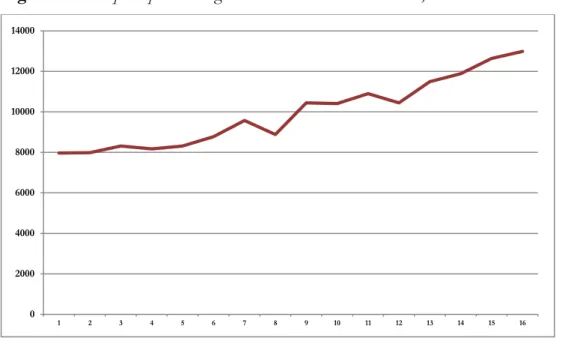
When analyzing the HDI trend for the sample of Latin American countries under study, it can be seen in Figure 1 a constant increase, with a minimum index of 0.67 in the beginning of the period analyzed and a value of 0.74 in 2015.

Figure 1: HDI trend in Latin America, 2000-2015

Note: countries’ values are averaged to get the index for every year.

Source: Own elaboration based on United Nations Development Programme data.

Figure 2 shows the HDI average of each country during the period considered, and as it can be observed Chile leads with a high index that places the country among those with “very high human development”, followed by Argentina with an average index of 0.79, Uruguay with an index of 0.77, Panama, Costa Rica, Mexico, Brazil, and Ecuador with an index still associated to “high human development”, while Guatemala has the lowest value getting an average of 0.59 in the period analyzed. Also, Honduras, Nicaragua, Bolivia, El Salvador, Paraguay, Colombia, and Dominican Republic register average values lower tan 0.7, and thus fell into the category of “medium human development”

Figure 2: HDI average for each Latin America countries, 2000-2015.

0,62 0,64 0,66 0,68 0,7 0,72 0,74 0,76 1 2 3 4 5 6 7 8 9 10 11 12 13 14 15 16

(20)

13

Note: countries’ values are averaged over the 16 years to get the score.

Source: Own elaboration based on United Nations Development Programme data.

Despite the positive trend of the HDI during the 15 years under analysis, it should be noted that Latin America is a region that, to this day, stands out for problems such as inequality and poverty. As Carballo (2010) mentions, after many crises unleashed during the nineties and the beginning of the twenty-first century, the weakness of the development model of many of these countries has been exposed after having to coexist inequality and high poverty rates with constant economic growth.

Gross Domestic Product per capita (GDP pc): GDP per capita PPP (constant

2011 international $) is also consider as dependent variable, and it is usually defined as the annual average income that a citizen of a country would receive, as long as the national income is distributed equitably. More formally, the World Bank refers to GDP per capita as “the sum of gross value added by all resident producers in the economy plus any product taxes and minus any subsidies not included in the value of the products and converted to international dollars using purchasing power parity rates”. The studies that relate corruption and GDP per capita are still scarce; some of them are Mustapha (2014) and Mikaelsson and Sall ( 2014).

Focusing on the sample of Latin American countries considered in this study, the evolution of GDP per capita (constant in 2011 $) can be seen in the following figures. Figure

0 0,1 0,2 0,3 0,4 0,5 0,6 0,7 0,8 0,9 Argentina Bolivia Brazil Chile Colombia Costa Rica Ecuador El Salvador Guatemala Honduras Mexico Nicaragua Panamá Paraguay Peru Dominican Republic Uruguay

(21)

14 3 represents the average GDP per capita for the sample of countries and it can be seen an increase every year, that is, average per capita income of Latin American countries is positive and increasing during the period 2000-2015.

Figure 3: GDP per capita average evolution in Latin America, 2000-2015

Note: countries’ values are averaged to get the index for every year. Source: Own elaboration based on World Bank data.

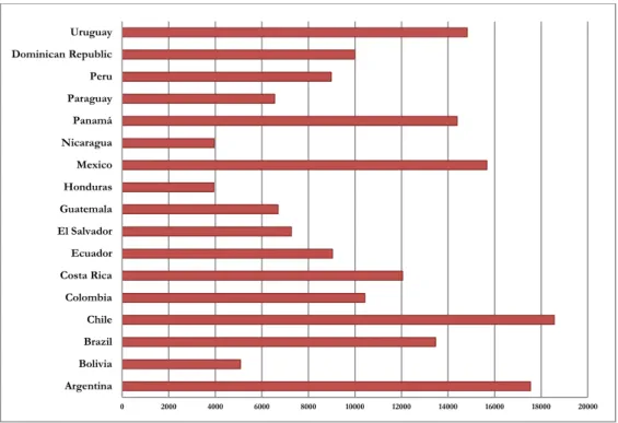
The following figure shows the average GDP per capita for each country during the 16 years under analysis. It can be appreciated that Chile, on average reached the highest GDP per capita, followed by countries such as Argentina, Mexico, and Uruguay. On the bottom, Honduras with an average of 3938 dollars is the country that obtained the lowest GDP per capita (see Appendix 3 for a detailed analysis).

Figure 4: GDP per capita average for each Latin American country, 2000-2015.

0 2000 4000 6000 8000 10000 12000 14000 1 2 3 4 5 6 7 8 9 10 11 12 13 14 15 16

(22)

15

Note: countries’ values are averaged over the 16 years to get the score. Source: Own elaboration based on World Bank data.

Independent variable:

Corruption: As stressed by Seligson (2006b), the Corruption Perception Index

(CPI) is one of the most used indicators in empirical studies focused on the impact of corruption (e.g., Mo (2001), Akçay (2006), Carballo (2010), Aidt (2009) , Oni and Awe (2012), Mustapha (2014)). For that reason, and because this index is available for the years and for the sample of countries selected this study also employs CPI.

Analyzing the evolution of CPI in a period of 16 years from 2000 to 2015 (Figure 5), it can be seen that on average Latin America had a poor performance over the period under study, with no considerable improvement being made. It can be noted that the highest average was in 2000 with a score of 37 on a total scale of 100, but subsequently its score was slightly decreasing reaching the minimum of 30 in 2011 and ending 2015 with an average score of 34.

Figure 5: CPI evolution in Latin America, 2000-2015

0 2000 4000 6000 8000 10000 12000 14000 16000 18000 20000 Argentina Bolivia Brazil Chile Colombia Costa Rica Ecuador El Salvador Guatemala Honduras Mexico Nicaragua Panamá Paraguay Peru Dominican Republic Uruguay

(23)

16

Note: countries’ values are averaged to get the index for every year. Source: Own elaboration based on Transparency International data.

Figure 6 depicts the average obtained for each Latin American country during the 15 years considered. On average, the country with the worst performance is Paraguay with a minimum of 23 points, followed by other countries such as Ecuador, Nicaragua, Honduras, Guatemala, Bolivia and Argentina that, on average, did not reach 30 points for the period under study. Chile and Uruguay have been the countries with the best performance in terms of this indicator. These two countries stand out for their good practices and up to now are located in the scale of this indicator in a more favorable position than even some advanced countries.

Figure 6: CPI average for each Latin American country, 2000-2015.

0 5 10 15 20 25 30 35 40 1 2 3 4 5 6 7 8 9 10 11 12 13 14 15 16

(24)

17

Note: countries’ values are averaged for 16 years to get the score. Source: Own elaboration based on Transparency International.

The improvement in this index has been scarce during the range of years analyzed in most countries (see Appendix 4), and despite the small advances in strategies to combat corruption in some Latin American countries, corruption remains one of the great of this region (Lipton et al., 2017).

Despite the difficulty of measuring corruption, with measures relying largely on perception, many scandals of corruption have come to light in recent years in this region. The report by Casas-Zamora and Carter (2017) describe different corruption scandals such as: the most notable as the Petrobras and Odebrecht case, one of the great massive bribery scandal that spread across South America; in Mexico, cases of corruption jolting the administration of the Mexican president Peña Nieto; in Guatemala, the resignation and arrest of President Otto Peres Molina after the revelations of a scheme of bribes in the customs agency; in Honduras, a financial crisis at the Honduran Social Security Institute (IHSS) due mainly to the misuse of funds from the national insurance system that is administered by the government; in one of the most transparent countries in Latin America, Chile, some problems with tax evasion, illicit campaign finance, and the misuse of political privilege. Therefore, during the last years, many corruption scandals have appeared in the headlines with disturbing regularity, highlighting the systemic corruption that prevails

0 10 20 30 40 50 60 70 80 Argentina Bolivia Brazil Chile Colombia Costa Rica Ecuador El Salvador Guatemala Honduras Mexico Nicaragua Panamá Paraguay Peru Dominican Republic Uruguay

(25)

18 in Latin America and the different ways in which this phenomenon affects society, such as the misappropriation of public funds or their fun, bribes that reach high political levels, cases of nepotism, among others.

Control Variables:

When analyzing the impact that corruption has on growth and economic development, it is necessary to control other possible variables that are determinants of economic development (Akçay, 2002). Thus, in line with studies such as those of Akçay (2006), Mikaelsson and Sall ( 2014) and Aidt (2009), control variables are included in the different econometric models, taking into account the level of correlation between them.

GDP per capita lag 5 years:GDP per capita lag is the GDP per capita with a lag of 5 periods.This variable is included to control the initial state of economic development of the countries. As it was mentioned in section 3, per capita income expectations of Latin American countries are positive and growing during the period 2000-2015, and thus it is expected a positive estimated sign for this variable.

Investment rate: Gross capital formation as the percentage of GDP is used to

measure the investment rate. Data is extracted from the World Bank database and is defined as “outlays on additions to the fixed assets of the economy plus net changes in the level of inventories”. According to the World Bank, fixed assets include improvement of routes, plant, machinery and equipment purchases, and the construction of roads, railways, and the like, including schools, offices, hospitals, private residential dwellings, and commercial and industrial buildings.

Human capital: The expected years of schooling is used as a proxy variable for

HumanCapital. Data comes from the United Nations Development Programme database

and, it considers the number of years of schooling that a child of school entrance age can expect to receive if prevailing patterns of age-specific enrolment rates persist throughout the child´s life.

Manufacturing share: The value added of manufacturing as the percentage of

GDP is gathered from the World Bank database. Manufacturing refers as industries belonging to ISIC division 15-37.2_{In a study carried out by Kaldor (1975), the author}

2_{International Standard Industrial Classification (ISIC) refers to the “physical or chemical transformation of}

materials of components into new products, whether the work is performed by power- driven machines or by hand, whether it is done in a factory or in the worker's home, and whether the products are sold at wholesale

(26)

19 concludes that there is a relationship between manufacturing output, and economic growth and this conclusion later led to what is known as the Kaldor´s first law that state that “manufacturing is the engine of growth”

Trade openness: This variable refers to exports plus imports as percent of GDP

and the data comes from the World Bank database. Many studies argue that a country can obtain great advantages from the trade openness through productivity improvement, enhance in resources allocation, investment and innovation.Barro and Sala-i-Martin (1997) show that international trade can have a positive impact on growth and the main reason is because it facilitates the dissemination of knowledge and technology of direct import or high-tech products.

Urban Population: Urban Population as the percentage of Total Population is

taken from the World Bank database and it refers to people living in urban areas. According to Perkins et al. (2013), a decline of the agricultural sector implies a substantial migration of labor from rural to urban areas in a country. Thus, urbanization can be an indicator for structural change and there should be a positive correlation between the level of urbanization of a country and the standard of living.

Gini: The Gini coefficient measures the inequality in income distribution of the

residents of a country. It measures the area between the Lorenz curve and the line of absolute equality, expressed as a percentage of the maximum area under the line. Thus, the Gini coefficient ranges from 0 to 1, where 0 represents perfect equality and 1 implies perfect inequality. According to economic literature, on one hand, income and wealth inequality may be, to a certain extent, beneficial and necessary in order to achieve rapid economic growth. Authors such as Forbes (2000), Partridge (1997) and others suggest that inequality is beneficial for economic growth. On the other hand, other studies establish that an increase in unequal income and wealth may have a negative effect on GDP per capita in relatively wealthy countries and a positive effect in poor countries (Galor and Zeira (1993)).

World Governance Indicators: They are an aggregate and individual indicators

presented by the World Bank and include six dimensions on governance such as (i) voice and responsibility, (ii) political stability and absence of violence, (iii) government

or retail. Included are assembly of component parts of manufactured products and recycling of waste materials. https://stats.oecd.org/glossary/detail.asp?ID=1586

(27)

20 effectiveness, (iv) regulatory quality, (v) rule of law and (vi) control of corruption. In this study, we consider the average of the first five dimensions and we exclude the dimension control of corruption, since it can be considered an alternative to the main independent variable CPI.

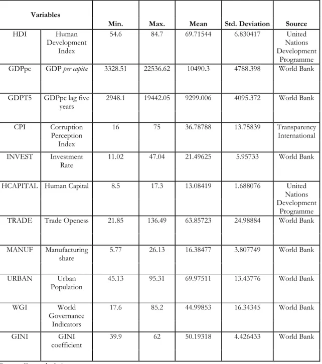
After describing all the variables considered in this study, the following table presents the main descriptive statistics of them.

Table 1: Descriptive Statistics

Variables

Min. Max. Mean Std. Deviation Source

HDI Human Development Index 54.6 84.7 69.71544 6.830417 United Nations Development Programme GDPpc GDP per capita 3328.51 22536.62 10490.3 4788.398 World Bank

GDPT5 GDPpc lag five

years 2948.1 19442.05 9299.006 4095.372 World Bank CPI Corruption Perception Index 16 75 36.78788 13.75839 Transparency International INVEST Investment

Rate 11.02 47.04 21.49625 5.95733 World Bank HCAPITAL Human Capital 8.5 17.3 13.08419 1.688076 United

Nations Development

Programme TRADE Trade Openess 21.85 136.49 63.85723 24.98884 World Bank

MANUF Manufacturing

share 5.77 26.13 16.38477 3.807749 World Bank

URBAN Urban

Population 45.13 95.31 69.97511 13.43776 World Bank

WGI World

Governance Indicators

17.6 85.2 44.99853 16.34345 World Bank

GINI GINI

coefficient 39.9 62 50.19318 4.426433 World Bank Source: Own calculation.

(28)

21 With 11.02% of GDP, Bolivia achieved the minimum percentage in terms of the Gross Capital Formation in 2004; however, in 2014 Panama stood out with a maximum of 47.04%. The expected years of schooling that a child can expect to receive was only 8.5 years for Guatemala in 2000, considered as the minimum expectation in the sample. Subsequently it was improved, until achieving an expectation of 10.7 years in the last year of analysis. Nevertheless, this country continues with the worse performance. In contrast, Argentina was the country that achieved a greater value about 17.3 for four consecutive years, from 2012 until 2015 years.

As for trade openness, Argentina is the country with the lowest percentage with 21.85% of GDP in 2001, which subsequently increased considerably until 2011 and then again decreased to 22.8% in 2015. Furthermore, Honduras had the highest percentage of

openness trade with 136.49% in 2005.The minimum percentage of manufacturing share is

5.77%, and it was observed by Panama in 2015. On the other hand, the maximum percentage of manufacturing share was reached by the Dominican Republic with 26.13% in 2000; however, the percentage of manufacturing share decreased in the Dominican Republic in the following years, finishing with 15.25% in 2015. In what concerns the percentage of urban population, 2000 registers the minimum value for Guatemala, 45.13%.

The maximum value, 95.31%, was reached by Uruguay in 2015, acountry that, along with

Argentina, during the 15 years of analysis has exceeded 90 percent of urban population. With respect to the World Governance indicators, Ecuador obtained the minimum score in the whole sample 17.6 in 2005 and Chile obtained the maximum score of 85.2 in 2004. Between 2000 and 2013 an excellent performance can be observed in Chile about this indicator with scores that exceeds 80 points, however, in 2014 and 2015 Chile registered a worse performance and finalized with a score of 61 in 2015. In 2000 Bolivia obtained the highest coefficient 61.6 in terms of income distribution between individuals and households that means a very high inequality level. Uruguay reached the lowest value of Gini coefficient 39.9 points in 2012, meaning that the lower inequality level for the sample under study was registered in this country for that year.

(29)

22

Chapter 4. The influence of corruption on the economic development of

Latin American countries: an empirical assessment.

In this chapter we present an empirical assessment of the impact of corruption on economic development, after controlling for other variables. We start by estimating the model using the methodology described in previous chapter, and then we proceed with the discussion of the results.

4.1 Correlation analysis

Considering the set of independent variables as well as dependent variables showed in previous chapter, we start by computing the correlation between the different variables that are used for this study. Values above 0.75 are interpreted as a high correlation or strong correlation between variables. As the table depicts, the situation of high correlation correspond to the following cases: between urban population and human capital (0.8205); between urban population and GDPT-5 (0.8484); and between world governance indicator and CPI the correlation (0.8867). Since the regression is likely to present multicollinearity problems when there is high correlation between independent variables, we avoid considering at the same time those variables that show high correlation in the same estimation specification.

Table 2: Correlation matrix among independent variables

GDP-5 CPI INVEST HCAPITAL TRADE MANUF URBAN WGI GINI

GDP-5 1.000 CPI 0.5824 1.000 INVEST 0.0601 0.0877 1.000 HCAPITAL 0.6769 0.4426 -0.1581 1.000 TRADE -0.5063 -0.1369 0.2124 -0.4990 1.000 MANUF -0.1818 -0.1689 -0.1702 -0.2608 0.1726 1.000 URBAN 0.8484 0.6140 -0.0285 0.8205 -0.6583 -0.2346 1.000 WGI 0.6344 0.8867 0.0334 0.4253 -0.1565 -0.0632 0.6097 1.000 GINI -0.4085 -0.3046 -0.0216 -0.3817 0.0663 0.0023 --0.3695 -0.2507 1.000

(30)

23

4.2 Results and discussion

Subsequently, we proceed with the estimation of a balanced panel data in which the number of countries is larger the years, N>T. In order to analyze the effect of corruption on economic development, six models with different combinations of independent variables were performed. First, the different models are estimated by Fixed Effect model (FEM) and Random Effect Model (REM). Subsequently, the Robust Hausman test is performed to decide which estimation model should be used. We must noted that the Robust Hausman test, unlike Hausman test , extends directly to heteroskedastic and cluster robust versions (Schaffer & Stillman, 2006). The null hypothesis of the Robust Hausman test is that REM is consistent. A large value of the test statistic (or a small p-value of the statistic) is a rejection of that null hypothesis, meaning that REM is inconsistent. Thus, with p-value less than 0.05 FEM estimators would be better.

GDP per capita as dependent variable

Table 3 shows the results of the estimations considering as dependent variable GDP per capita. The results of Sargan-Hansen statistic indicates that for models II, III, IV and VI with a p-value less than 0.05, the null hypothesis of "REM consistent" is rejected; however, for models I and V the null hypothesis is not rejected and so these specifications are estimated using "REM". When considering the R-squared value, the results indicate that the overall fit is high for all models. Particularly, for model III and V the fit indicates that 97% of the total variation in GDP per capita is explained by the independent and control variables. As it can be observed in table 3, the main independent variable - the CPI - is not statistically significant in model IV but it is for the other specifications. The base model, that is model I, shows that an increase in the CPI scale, meaning a higher control of corruption, has a positive impact on GDP per capita in Latin American countries.

The GDP per capita incorporated as a 5 years lag variable is strongly significant in the different regressions. The investment rate, proxy for the gross capital formation, is strongly significant in the different models when this variable was incorporated as control variable, being positively correlated with GDP per capita. According to model II, for every increase in investment rate, GDP per capita will improve significantly. The Human capital variable that refers to the expected years of schooling is considered in four models as control variable and only in two it has a significant and positive estimated effect. In model II, one year increase in the expected years of schooling, implies an estimated increase of 265 dollars in GDP per capita, ceteris paribus.

(31)

24

Table 3: Corruption and economic development I: Latin America, 2000-2015 Explained variable: GDP per capita

Control and Explanatory

variables Model I (RE) Model II (RE) Model III (RE) Model IV (FE) Model V (RE) Model VI (FE)

CONST _-1044.4

(0.008) -6364.568 (0.000) 2015.516 (0.267)

5507.151

( 0.303) -513.951 _(0.824) 4514.252 _(0.353)

GDP-5 GDP per

capita lag five

years 1.075 (0.000)*** (0.000)*** 0.958 (0.000)*** 0.915 (0.027 )** 0.606 (0.000)*** 0.859 (0.029)** 0.608 CPI Corruption Perception Index 42.249 (0.037)** _(0.001)***39.699 _(0.000)***30.899 _{(0.579 )}-13.375 _(0.001)***24.141 INVEST Investment rate 141.008 (0.000)*** (0.000)*** 139.394 (0.004)*** 146.311 (0.000)*** 107.291 (0.005)*** 142.623 HCAPITAL Human capital (0.046)** 265.431 (0.017)** 281.788 365.860 (0.121) 366.0097 (0.139) TRADE Trade Openess -13.127 _(0.298) _(0.751)-2.264 -11.155 _(0.400) MANUF Manufacture share -65.46986 (0.353) -66.009 _(0.335) URBAN Urban population _(0.001)***58.303 WGI World Governance indicatos 5.113 (0.628) GINI Gini coefficient (0.055)* -74.390 - 119.565 ( 0.082)* (0.052)* -81.557 -115.632 (0.084)* Summary statistics Sargan-Hansen statistic 2.642 (0.2668) (0.0560) 9.214 (0.0745) 10.025 (0.0215) 16.424 (0.1054) 10.492 (0.0310) 15.419 R-squared 0.95 0.96 0.97 0.93 0.97 0.94 Wald test 873.24 (0.0000) (0.0000) 2378.84 (0.0000) 2063.08 (0.0000) 2488.00 F-statistics 45.75 (0.0000) (0.0000) 39.67 N° of groups 17 17 17 16 16 16 N° of observations 264 264 235 217 220 218

Note: p-values in parenthesis, significance level at 1% (***), 5% (**) and 10% (*).

Trade openness shows an estimated negative association with GDP per capita that is not in line with studies such as Barro and Sala-i-Martin (1997) but this control variable effect is not statistically significant. The variable manufacturing share included in two specifications also shows a negative correlation with GDP per capita but its effect is also not statistically significant. The World Governance Indicator that, as mentioned, represents the

(32)

25 average of five dimensions (voice and responsibility, political stability and absence of violence, government effectiveness, regulatory quality, rule of law) is not statistically significant. Urban population that is incorporated only in model V is strongly statistically significant and with the expected positive effect on GDP per capita as some empirical studies states such as Perkins et al. (2013) and Akçay (2006). The result indicates an increase in urban population rate has a significant estimate effect on GDP per capita. And, as for the last control that is Gini coefficient, a statistical significant effect emerges at 10% level of significance for a negative estimated effect on GDP per capita indicating that although this result is slightly significant , it is in the line with authors previously mentioned as Forbes (2000), Partridge (1997) and others who mention that inequality is beneficial for economic growth. In model IV, where we can see the highest estimated effect of inequality, the result shows that when the Gini coefficient increases by one point, GDP per capita decreases by 119.565 dollars.

HDI as dependent variable:

Table 4 shows the different estimations considering "HDI" as the dependent variable. The Sargan–Hansen test indicates that the REM should be used to run models I and II, whilst for the remaining models the FEM is better. Considering the R-squared value, it is noted that the variation in the HDI is explained by more than 80% by the variables considered in the model, showing that the variation for each one in terms of R-squared is high.

As it can be seen in the different estimations, the effect of the CPI is statistically significant in models I, II and V and all of them show a positive correlation with the HDI. According to the first estimated model that show the direct effect of corruption perception index without any control variable, a 1% increase in the scale of this index has a positive estimated effect of 0.112 points on HDI. In models II and V, as expected, the estimated effect of the CPI is reduced when control variables such as the investment rate, human capital and urban population are incorporated in the different models.

(33)

26

Table 4: Corruption and economic development II: Latin America, 2000-2015 Explained variable: HDI

Control and Explanatory

variables Model I (RE) Model II (RE) Model III (FE) Model IV (FE) Model V (FE) Model VI (FE)

CONST 53.536 (0.000) (0.000) 31.670 (0.000) 58.652 (0.000) 57.752 (0.044) 18.759 (0.000) 60.316 GDPT-5 GDP per capita lag five years 0.0013 (0.000)*** (0.000)*** 0.0006 (0.014)** 0.0003 (0.001)*** 0.0003 (0.001)*** 0.0003 (0.013)** 0.0003 CPI Corruption Perception Index 0.112 (0.000)*** (0.027)** 0.086 (0.529) 0.021 (0.423) 0.026 (0.054)* 0.071 INVEST Investment rate (0.007)*** 0.105 (0.052)* 0.056 (0.001)*** 0.068 (0.021)** 0.092 (0.028)** 0.063 HCAPITAL Human capital (0.000)*** 2.027 (0.000)*** 1.613 (0.000)*** 1.703 (0.001)*** 1.574 (0.000)*** 1.614 TRADE Trade Openess (0.310) 0.011 (0.448) 0.008 MANUF Manufacture share (0.138) -0.096 (0.126) -0.095 URBAN Urban population (0.040)** 0.315 WGI World Governance indicatos -0.010 (0.492) GINI Gini coefficient (0.000)*** -0.282 (0.000)*** -0.311 (0.000)*** -0.288 Summary Model Sargan-Hansen statistic 1.081 (0.5826) (0.1645) 6.504 (0.0000) 149.681 (0.0000) 65.239 (0.0006) 21.754 (0.0009) 78.556 R-squared 0.84 0.90 0.86 0.83 0.84 0.84 Wald test 116.81 (0.0000) (0.0000) 479.55 F-statistic 205.99 (0.0000) (0.0000) 241.56 (0.0000) 187.74 (0.0000) 167.43 N° of groups 17 17 16 17 17 16 N° of observations 264 264 217 235 264 218

Notes: p-values in parenthesis. Significance level at 1% (***), 5% (**), and 10% (*).

With respect to the investment rate, the estimations of models II and IV show that its estimated effect strongly significant, statistically significant at 5% in models V and VI, and at 10% in model III. In model II, the estimation result shows that an increase of 1% in the investment rate generates a positive effect on HDI by 0.105 points. The estimates associated to human capital are strongly statistically significant in the different models and the different results show a positive association with HDI. In model II, the estimated

(34)

27 coefficient associated to human capital indicates that for every 1 year increase in the expected year schooling, HDI improves by 2.027 points. Trade openness incorporated as a control variable in two models does not have a statistically significant impact. Also, the results for the manufacturing share variable that is included in two estimation models are not statistically significant.

Urban population is statistically significant at 5% in the only model where it is included and the result shows that an increase in the urban population rate generates an improvement in HDI. The World Governance Indicator is not statistically significant, whereas the last control variable – the Gini coefficient - the different estimations in the models III, IV and VI that include this variable show that this variable is strongly statistically significant and with a negative estimated effect on HDI. For each 1 point increase in the Gini coefficient that means an increase in inequality, the HDI decreases by 0.282 points for Latin American countries under study.

As mentioned earlier (see chapter 2), most empirical studies that analyze the impact of corruption on different macroeconomics variables such as Akçay (2006), Carballo (2010) that studies the impact of corruption on human development and poverty or studies focused on the impact of corruption on economic growth such as Akçay (2002), Mauro (1995), Mo (2001), Aidt (2009), Vaal and Ebben (2011), Ahmad et al. (2012), Pulok (2012), Oni and Awe (2012), Mikaelsson and Sall ( 2014), Mustapha (2014), conclude that corruption can be seen as a factor that impacts negatively on the economy through different mechanisms.

The main objective of the different estimations carried out in the present dissertation is to determine the effect of corruption on human development and GDP per capita. The results show a negative effect on both variables which is in line with many of the conclusions to which most of the empirical studies arrived such as studies of Tanzi and Davoodi (1997), Mo (2001), Akçay (2006), Akçay (2002), Aidt (2009) among others. (The results also sustain that the most commonly control variables identified in the related literature as determinants for economic growth such as the investment rate (proxy for gross capital formation), human capital (the expected years of schooling as proxy) and urban population, together with corruption, are important determinants of human development which is in line with the results reached by Akçay (2006). Also, when considering the GDP per capita variable, it is observed that these variables have a significant estimated effect on this variable.

(35)

28

Chapter 5: Conclusions

Several decades ago corruption was a phenomenon analyzed mainly by political scientists, sociologists, historians. Approximately since the nineties a greater interest in the topic of corruption started to emerge among economists who began considering corruption as a variable of interest for the study of economic growth and development. However, as literature review shows, empirical studies that assess the effects of corruption on economic development are still scarce (e.g. Akçay (2006), Carballo (2010)) especially for the Latin American region. Therefore, the main purpose and goal of the present dissertation has been to fill in this gap, by determining the effect of corruption not only on GDP per capita but also on human development, considering a sample of 17 Latin American countries over a period of 16 years. The conclusions of this study are the following:

First, after carrying out several regressions taking into account the impact of corruption on two alternative dependent variables, GDP per capita and human development, the main conclusion that has been reached is that corruption has a negative estimated effect on both variables for the sample of the 17 Latin American countries over the period 2000- 2015. This result goes in line with the study of Akçay (2006), one of the few studies that analyzed corruption and human development.

Second, the data on the CPI indicates that most of the analyzed countries with the exception of Chile and Uruguay, have been scored below 50 on a scale of 0 (highly corrupt) to 100 (highly transparent) during the period analyzed. Also, the level of corruption for the Latin American countries was maintained during the 15 years without significant improvement. Regarding this aspect, Chile, Uruguay and, to a large extent, Costa Rica stand out for their good performance in the corruption perception scale with a score similar to many developed countries.

Third, an average of 0.7 for HDI was reached for the sample of countries as a whole during the period under consideration, falling within the category “high human development”. However, Chile stood out during the period, which led it to be placed within the category of countries with "very high human development". Finally, in terms of GDP per capita, Argentina, Chile and Mexico showed the highest average GDP per capita in