and its components
Jair Andrade Araujo, Débora Gaspar Feitosa
and Almir Bittencourt da Silva
ABSTRACT This article applies the stochastic-frontier model to examine total factor productivity (TFP)
and its components in Latin America between 1960 and 2010. The likelihood-ratio test
shows that, for a selection of Latin American countries over the 50 years analysed, the
macroeconomic variables of technical inefficiency included in the model generally have
a significant effect; and they allow for a better understanding of technical inefficiency
throughout the region. The key variables explaining technical inefficiency in the selected
countries are public expenditure and the inflation rate; and there is also an inverse
relation between technical inefficiency and the extent to which local prices diverge from
purchasing power parity.
KEYWORDS Productivity, measurement, mathematical analysis, econometric models, Latin America
JEL CLASSIFICATION O47, O54, O57
AUTHORS Jair Andrade Araujo has a Ph.D. in Economics and is a Professor on the Masters Course in Rural Economics
(maer) of the Federal University of Ceará (ufc), Brazil. [email protected]
Débora Gaspar Feitosa has a Ph.D. in Economics and is a Professor on the Economic Sciences and Finance Courses of the Federal University of Ceará (ufc), Brazil. [email protected]
Using the concept of total factor productivity (tfp), quantified using the Cobb-Douglas production function, Solow (1957) introduced the measurement of the contribution made by technical progress to per capita output growth. This author estimated the production function of the United States economy from 1909 to 1949, and established the existence of a residual, measured as the difference between the growth rates of real output and the weighted growth rates of the individual factors of production, capital and labour. The importance of technical progress, which was discovered when attempting to break down the growth rate of real output using the growth rates of the factors of production, is known as the Solow residual.
The notion of technical progress then came to be used as an abbreviated expression for any shift of the production function. Nonetheless, based on empirical studies founded on growth accounting and inspired in the neoclassical model, some authors started to claim that several causes could be closely related to the measurement of the residual. Drawing on Solow’s work, a number of empirical studies were performed —such as those of Griliches (1996), which uses various methodologies and samples— aimed at analysing the components of the aforementioned residual, with a view to quantifying as precisely as possible the real contribution that technical progress makes to output growth.
Orea (2002) studies panel data based on information from Spanish banks and proposes a parametric breakdown of the Malmquist index. The results show that tfp growth can be attributed mainly to technical progress. Färe, Grosskopf and Roos (1998) also study productivity and the Malmquist index. The empirical studies of Färe and others (1994); Johnson and Kuosmanen (2012); Lee and others (2013), and Wang and others (2014), among various authors, also show that it is possible to study the productivity of economic agents using non-parametric or semi-parametric methods. For example, data envelopment analysis (dea) is a non-parametric methodology that can be used to evaluate the technical efficiency of productive units and estimate the Malmquist index.
The present article reports an application of the tfp decomposition procedure suggested by Bauer (1990) and Kumbhakar (2000) to a sample of Latin American countries for the period 1960-2010, based on the stochastic production-frontier model. The advantage
of this approach is that allows tfp to be broken down into components that characterize the general production process. The procedure used makes it possible to identify the components of technical efficiency, which reflect the way an economy moves towards the production frontier, as distinct from the technical progress component, which represents a shifting of the frontier itself.
An advantage of the procedure used by Bauer (1990) and Kumbhakar (2000) is that by permitting a flexible specification of the production frontier, such as translog, tfp can be broken down into the components of technical efficiency, allocative efficiency, scale effect and technical progress. This procedure is superior to decomposition using the tfp Malmquist index (based on a production frontier that is restricted by the imposition of constant returns to scale), which is used in many other studies. In this case, according to Färe and others (1992), tfp is divided into just two elements: the variation in technical efficiency and technological change. This line of research also includes studies by Kumbhakar and Lovell (2003); Sauer, Frohberg and Hockmann (2006), and Henningsen and Henning (2009).
This article uses the stochastic-frontier model to analyse the contribution made by tfp to economic growth in a sample of Latin American countries; for which purpose it examines the components of technical efficiency, allocative efficiency, scale effect, and technical progress in the variation of tfp in those countries. It thus contributes to the empirical literature for a better understanding of the real factors that underlie the economic performance of the sample countries over a 50-year period. A further aim is to understand the influence of the vector of macroeconomic variables on the technical efficiency of the countries in the sample, through the technical inefficiency model, following Battese and Coelli (1995).
The article is divided into six sections including this introduction. Section II briefly explains the stochastic-frontier model and the tfp decomposition procedure; and section III presents the databases, sample of countries and the econometric model used. Section IV demonstrates the calculation of the tfp decomposition, using the Bauer (1990) and Kumbhakar (2000) procedure; and section V presents the results of the estimation and breakdown. The sixth and last section puts forward a number of final thoughts.
I
II
Stochastic frontier and
TFP
decomposition
This study uses stochastic production-frontier analysis, which is one of the methods adopted in the technical-inefficiency literature, to identify one of the components of tfp, namely technical efficiency.
The approach uses econometric (parametric) techniques, whose production-frontier models are used to study technical inefficiency, and it is recognized that output can be affected by random disturbances that are outside producer control. Unlike non-parametric approaches, which assume deterministic frontiers, stochastic-frontier analysis allows for deviations from the frontier, for which the error can be broken down into changes in technical efficiency and random disturbances.
In the deterministic-frontier models, deviations from the production frontier are attributed to the producer’s technical inefficiency; but those models ignore the fact that production can be affected by random disturbances outside producer control, such as strikes or environmental conditions, among others.
Stochastic-frontier analysis originated in articles by Aigner, Lovell and Schmidt (1977) and Meeusen and Broeck (1977), which were followed by the work of Battese and Corra (1977). Those original studies present the structurally composed error term in the context of the production function. Since then, various authors have collaborated, including Battese and Coelli (1995), who modelled technical inefficiency as time-variant, formalizing the technical inefficiency of the stochastic production function for panel data. The present article adopts the model proposed by Battese and Coelli (1995) and Coelli, Rao and Battese (1998). Accordingly, the stochastic production-frontier model can be described through equation (1), where yit is the
vector of quantities produced by the various countries in period t; xit is the vector of factors of production used
in period t, and β is the vector of parameters defining the production technology.
, , . . ,
, ..., , , ...,
exp exp
y f t x v u u
i N t T
0
1 1
it= itb it − it $
= =
_ i _ i _ i (1)
The terms vit and uit are vectors that represent
different error components. The first relates to the random part, with a truncated normal distribution, independent and identically distributed, with a constant
variance of σ2, (v ~ iid N (0,
v
2
v )); whereas the second represents technical inefficiency, in other words the part that constitutes a retreat from the production frontier, which can be inferred from the negative sign and the constraint u ≥ 0. These are non-negative random variables with a zero-truncated normal distribution, independently distributed (not identically) with mean μit and constant variance vu2; in other words (u ~ NT (μ,vu2)). As the
error components are mutually independent and xit is assumed exogenous, the model can be estimated using the maximum-likelihood technique.
Unlike the model used by Pires and Garcia (2004), this one has the advantage of allowing inefficiencies and input elasticities to vary through time, which makes it easier to identify changes in the production structure.
The effects of technical inefficiency (eit) are expressed with the following characteristics:
eit = zitδ + wit
where: zit is a vector of explanatory variables of the technical inefficiency of the i-th productive unit (country) measured in time t; δ is a vector of parameters associated with the variables zit; and wit is a normally distributed random variable with zero mean and variance vw2. It is assumed that eit has a zero-truncated normal distribution, so its mean is wit = zitδt .
Under this formulation, a functional form is defined, as presented below; and this is used to obtain tfp, which is then broken down into its components.
III
Methodology
1. Description of the sample and the data used
The analysis considers the following 19 Latin American countries: Argentina, the Bolivarian Republic of Venezuela, Brazil, Chile, Colombia, Costa Rica, the Dominican Republic, Ecuador, El Salvador, Guatemala, Honduras, Jamaica, Mexico, Nicaragua, Paraguay, Peru, the Plurinational State of Bolivia, Trinidad and Tobago, and Uruguay. The data relate to the period 1960-2010, and were obtained from the following sources: Penn World Table 7.1 (pwt 7.1) and the World Development Indicators published by the World Bank. The availability of information from those databases was decisive in choosing 2010 as the upper bound of the sample.
The variables gross domestic product (PIB), labour (L), government consumption expenditure (G) and deviation of local prices from purchasing power parity (DPPA) were taken from Penn World Table 7.1. The series for physical capital (K) of the individual countries was constructed from estimates based on gross investment, using the perpetual-inventory technique.
The inflation rate data came from the World Development Indicators, although the difficulties in obtaining data for certain countries meant that other sources were also used. In the case of Brazil, the general price index-domestic supply (igp-di) published by the Getulio Vargas Foundation was used.
The sample consists of annual data on capital, labour, gdp, government expenditure, purchasing power parity and inflation from the 19 selected countries, totalling 950 observations forming a balanced panel.
2. Econometric model
Total factor productivity was calculated using the stochastic production-frontier model proposed by Aigner, Leobel and Schmidt (1977) and Meeusen and Broeck (1977), which was subsequently improved by Pitt and Lee (1981) and Schmidt and Sickles (1984). This makes it possible to model the panel data with the productive technical-inefficiency component, according to the foundations used by Battese and Coelli (1995), which suggest that technical inefficiency is modelled by a vector of variables.
This being the case, a functional form of the production frontier is modelled, in conjunction with a
hypothesis about the distribution of technical inefficiency (Battese and Coelli (1995)).
Firstly, one model was tested using the Cobb-Douglas functional form and another using the translog form. The adequacy test identified the latter functional form as superior in terms of data consistency.
Accordingly, the translog production-frontier function for the 19 selected Latin American countries was specified as follows:
t LnK tLnK
LnL tLn LnK Ln
LnK LnL v u
LnY t
L L
2 1
2 1
2 1
it it
it it it it
it it it it
it i 3 2 4 5
6 7 8 9
2
10 2
2
a a a
a a a a
a
a a + + +
+ + + +
+ + −
= +
_ i _ i (2)
where:
Yit = gdp of country i in period t.
Kit = physical capital stock of country i in period t.
Lit = labour in country i in period t.
ai= fixed effects, with the aim of capturing unobserved
heterogeneities in the sample of countries. t = linear trend.
t 2
1 2 = quadratic trend.
vit = random disturbances of the production function,
which are assumed to be normally distributed with zero mean and constant variance.
uit = technical inefficiency of production, modelled
as follows:
uit=dzit+~it (3)
where:
zit = (z1t, z2t, z3t, z4t) represents a vector of variables
that explain technical inefficiency, and δ is a parameter of associated with zit.
ωit = assumed normally distributed N(0,
2 v~).
Under the foregoing hypothesis, it is also assumed that uit is independently distributed in a truncated normal
distribution with mean wit = δzit, and constant variance
of v2~.
The inefficiency variables considered are as follows: z1t = trend effect.
z2t = government consumption expenditure relative to
the gdp of each country. Some empirical studies have been conducted to quantify the effect of current expenditure outgoings on inefficiency. For example, Bittencourt and Marinho (2007) analyse tfp in Latin American countries and discuss the effects of macroeconomic variables in explaining the technical inefficiency component through the stochastic frontier. They find that current government expenditure contributed to increasing technical inefficiency in the countries of the sample between 1961 and 1990. Thus, an increase in government expenditure would be expected to make production more technically inefficient.
z3t = corresponds to the logarithm of 1 + the inflation
rate, p, in other words ln (1 + p). This expression is used because it captures the non-linear effects of inflation on technical inefficiency. According to De Gregorio (1992), some countries experienced periods of deflation and hyperinflation, but the influence of those extreme situations on the inefficiency term is attenuated by using the expression indicated above. Inflation is expected to increase the technical inefficiency of production.
z4t = corresponds to the deviation of the local price level
from purchasing power parity, using the United States as the benchmark country. This variable serves above all to control for the technical-inefficiency effects of trade policies that involve devaluation of the real exchange rate.
The parameters of equations (2) and (3) are estimated using the maximum-likelihood method, which makes it possible to calculate the magnitude of technical efficiencies for each country in the sample.
3. Tests conducted
(a) Functional form
Firstly the Cobb-Douglas and then the translog production functions were estimated, for the purpose of using the adequacy test to choose which functional form to use in the study. Although the Cobb-Douglas functional form is commonly used in frontier-estimation models, it is a simple model with few properties, including constant elasticity and returns to scale (Coelli, Rao and Battese, 1998).
Thus, in line with several studies, the functional form test is used to estimate both the Cobb-Douglas and the translog forms; and the null hypothesis that
Cobb-Douglas is the appropriate form for presenting the data is tested, given the translog specifications. This can be tested using the likelihood-ratio test. The table published in Kodde and Palm (1986) is used to compare the critical values of the results, given the degrees of freedom. The test proceeds as follows:
After obtaining the two models and their respective maximum-likelihood ratios (ll), the generalized-likelihood statistic (lr) of the estimated production functions is considered. Then the hypothesis test is applied:
H0: LL Cobb-Douglas. H1: LL translog.
and, consequently, the generalized-likelihood ratio, LR = - 2 [ln LL H0 – Ln LL H1]
LR > T KP (Kodde and Palm, 1986 table) H0 is rejected.
To find an ideal model to represent the data, further functional form tests were conducted in addition to that described above between Cobb-Douglas and translog. These tests only changed some of the inefficiency variables, but owing to a lack of convergence between certain models, it was impossible to make comparisons.
(b) Absence of technical progress
This test considers whether or not the coefficients of the time-related variables in the translog function are equal to zero. In other words, it tests the hypothesis that a2, a3, a5, a7 in equation (2) are equal to
zero. Thus:
H0: a2, a3, a5, a7 = 0.
H1: complete translog.
Using the generalized-likelihood ratio, LR = - 2 [ln LL H0 – Ln LL H1]
LR > T KP (Kodde and Palm, 1986 table) H0 is rejected.
(c) Effect of technical inefficiency on the production function
This case tests for the nonexistence of technical inefficiency; in other words, whether in fact the inefficiency variables depend on the model. For that purpose, the log-likelihood value (ll) is taken of the model estimated without these variables, and the generalized-likelihood test is performed again, comparing it with the critical value of Kodde and Palm (1986). The degrees of freedom correspond to the inefficiency variables.
Thus:
(d) Absence of fixed effects
This test is used to evaluate the model without the presence of fixed effects captured by its dummy variables. The model is once again estimated without taking account of the presence of those dummy variables, and the generalized-likelihood test is applied,
with reference to the critical value of Kodde and Palm (1986).
In this particular study, the estimation without fixed effects did not converge after a large number of iterations, so the model could not be estimated and was rejected for comparison purposes.
IV
Decomposition of
TFP
1. Composition of the data
In order to break the tpf down into its components, the country data were used to develop the initial econometric model, along with the data calculated from that model.
The 19 countries of the sample were maintained for the econometric model, and the period 1960-2010 was maintained for the analysis, with data on capital (K), labour (L) and gdp (Y) mainly being used. The factor shares SK and SL were obtained from calculations based on Penn World Table 7.1 data.
The elasticities
e
k ande
L were calculated on the basisof the respective derivatives of the translog production function used in relation to the corresponding factors of production.
2. Decomposition procedure
Bauer (1990) and Kumbhakar (2000) proposed a productivity decomposition that goes beyond changes in productivity to capture the effects of technical innovation. This approach also takes account of production-scale effects. That decomposition is performed by firstly estimating the model of equations (2) and (3), after which it is possible to “compose” the rate of change of tpf based on the results.
According to that model, which was used by Pires and Garcia (2004), on the basis of the formulation proposed by Battese and Coelli (1993), it is possible to study the effects of each tpf component. The main advantage of this is that it admits the possibility of variable returns to scale.
In this way, the components of productivity can be identified after some algebraic manipulations on the expression that represents the deterministic part of the production frontier. Pires and Garcia (2004) present an index for the tpf growth rate expressed as:
g yy s
K K
s L L
PTF= − K − L
c c c
(4)
in the deterministic part, it can be seen that:
, , , ln y y
t f t K L
K K
L L
t u
K L
2 2
2 2
b
f f
= + + −
c _ i c c
(5)
where:
SK = the capital share of income; SL = the labour
share of income;
e
K = the elasticity of capital; ande
L = the elasticity of labour.Returns to scale (rts) are defined as the sum of elasticities, such that:
RTS =
e
K +e
Lwhere,
gK = growth rate of K
gL = growth rate of L
Setting, K RTS
K
m = f and L RTS
L
m = f , and substituting in the index, a number of algebraic operations are then performed:
.
. .
. . g
s g s g
g PT u RTS 1 g
K K K L L L
L L
PTF K K m
m m
m
+ − + −
= −c+_ − +
_ _
i
i i
7
9
A
C (6)
Equation (6) describes the rate of variation of tfp, gPTF, which can be broken down into four elements:
technical progress, variation of technical efficiency, variations in the scale of production, and variations in the efficiency of resource allocation.
, , , ln PT
t f t K L
2
2 b
= _ i
The change in technical efficiency is denoted by the technical inefficiency coefficient with a negative sign −uc.
It should be noted that the change in production scale is given by the expression that contains the returns to scale and growth rates of capital and labour, in other words the third term of equation (6): (RTS -1).[λK.gk + λL.gL].
Changes relating to allocative efficiency are represented by the last term in equation (6), which relates proportionate returns to scale, the shares of capital and labour, and the growth rates, and is thus measured by: [(λK - sk).gK + (λL - sL ).gL].
This methodology, with which productivity is broken down into the four components mentioned, makes it possible to evaluate the repercussion of each
one separately. For example, if technology does not change (if PT = 0 in the item defined above), this will not contribute to productivity gains. Similarly, technical inefficiency, which changes through time, will have repercussions on the rate of variation; otherwise, if
u 0
− =c = 0, it will not affect that rate.
With constant returns to scale (RTS = 1), the third component of the formula for the variation in productivity is zero. Nonetheless, if RTS ≠ 1 productivity can partially explain returns to production scale.
By setting λK + λL = 1, one can discern a symmetry
in the distances of the shares of K and L with respect to λ, where the capital and labour shares are symmetric and, consequently, have opposite signs. According to a reallocation factor, this means that the intensity of one factor will reduce the intensity of the other; in other words, that capital intensity will reduce the amount of labour, and vice versa.
1. Analysis of the estimation of the production frontier
Table 1 shows the model that corresponds to the estimation of the production frontier in the translog functional form, which was the model that best fit the data after the appropriate tests described above. All of the estimated parameters are statistically significant at the 5% level, except for the a2 of variable t, which did not return a conclusive result.
Nonetheless, the parameters of the stochastic production frontier estimated in terms of the trend components, provide clear evidence that technical progress occurred at an increasing rate (shown by the positive sign of the t2 variable, which is significant at 1%), which thus means an acceleration in the variation of technical progress.
The value of the technical inefficiency indicator,
g, is 0.51. This means that 51% of the total variance of the composed error of the estimation of the translog production function is explained by the variance in technical inefficiency. This makes it very important to incorporate technical inefficiency into the model.
Table 1 shows that all of the estimated parameters of the variables included to explain the technical inefficiency
V
Estimation and results
are statistically significant at the 1% level, and have the expected signs.
For example, the estimated coefficient of the trend variable (z1t) in the technical inefficiency model has a positive sign and is statistically significant at 1%, which could indicate a tendency for inefficiency to increase in the period studied.
The government current expenditure variable (z2t) is significant and has a positive sign, which suggests that the large share of current expenditure in the composition of aggregate spending in Latin American countries, on average, produces inefficiency in the economy. To some extent, these results agree with those obtained by Klein and Luu (2001), who concluded that countries with high levels of current expenditure tend to be less efficient, since a high level of public expenditure crowds out productive investments and thus generates distortions in resource allocation.
inflationary periods, which had negative repercussions on the technical inefficiency and development of their economies.
In the case of the variable that captures the deviation of local prices from purchasing power parity (z4t), the
estimated coefficient is significant and has the expected negative sign. This indicates that countries which adopted
TABLE 1
Results of the model in the transloga functional form, 1961-2010
Variables Estimations Z-value
d1 0.395 8.8
d2 -0.683 -13.5
d3 1.490 9.9
d4 -0.226 -8.2
d5 0.416 10.3
d6 -0.592 -7.9
d7 -0.475 -10.5
d8 -0.770 -24.6
d9 -0.540 -9.3
d10 -0.400 -9.5
d11 -0.930 -14.6
d12 -0.931 -13.6
d13 1.150 14.4
d14 -1.020 -13.0
d15 -1.073 -18.2
d16 -0.155 -5.5
d17 -0.844 -7.5
d18 -0.934 -16.8
t -0.014 -1.3
t 2 1 2
0.001 11.8
LnL 0.973 4.4
LnK -0.327 -2.2
tLnL 0.001 1.8
tLnK -0.002 -3.2
LnL ∙ LnK 0.061 5.8
LnL 2 1 2
_ i -0.069 -4.4
LnK 2 1 2
_ i
0.024 2.9
Constants 11.22 11.2
Z1-trend effect 0.018 4.3
Z2-government consumption expenditure 30.729 5.7
Z3-inflation rate 0.098 2.9
Z4-degree of openness -0.806 -3.4
Constants -0.696 -3.3
lnsigma2 -3.829 -17.7
Ilgtgama 0.042 0.93
sigma2 0.021
-gamma 0.510
-sigma_u2 0.011
-sigma_v2 0.010
-Source: prepared by the authors, on the basis of the research data.
a Number of observations: 950; log-likelihood probability: 729.28 and probability>chi-squared = 0.0000.
Note: the “d” variables represent the fixed effects of the countries. The other variables correspond to those indicated in equation (2). Gamma and sigma correspond to the results of the log-likelihood function expressed in terms of the parameterization specified
by
u v u 2 2
2
v v
c v
+
= .
2. Analysis of the hypothesis tests
Once the models had been estimated, the respective tests were conducted for functional form, the absence of technical progress and technical inefficiency.
Table 2 sets out some of the results. Firstly, the Cobb-Douglas functional form was tested in comparison with the translog model, and then the likelihood-ratio was used to verify the best functional form. This means testing
the hypothesis that all of the second-order coefficients and the coefficients of the cross-products of the function defined in (2) are equal to zero. It should be noted that the value of the likelihood ratio was 9.77, which is above the 7.04 critical level of the value statistic of Kodde and Palm (1986) (critical value to the right of the c2 distribution at 5% with 3 degrees of freedom). It can therefore be assumed that the most appropriate model for the problem under study is the translog functional form.
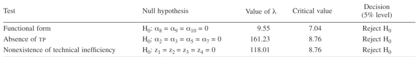
TABLE 2
Likelihood-ratio test of the parameters of the stochastic production frontier
Test Null hypothesis Value of λ Critical value Decision (5% level)
Functional form H0: a8 = a9 = a10 = 0 9.55 7.04 Reject H0
Absence of tp H0: a2 = a3 = a5 = a7 = 0 161.23 8.76 Reject H0
Nonexistence of technical inefficiency H0: z1 = z2 = z3 = z4 = 0 118.01 8.76 Reject H0
Source: prepared by the authors.
λ: Statistical test of the likelihood ratio in which λ = -2 {log [likelihood (H0)] – log [likelihood (H1)]}. This test has a roughly chi-squared
distribution with degrees of freedom equal to the number of independent constraints. tp: technical progress.
Once the functional form had been chosen, the absence of technical progress was tested. In line with the test described above, the model was estimated in the translog functional form, and with the absence of technical progress. The respective values of the log-maximum-likelihood of each estimation were used to obtain lr = - 2 [648.67 – 729.28] = 161.22. The result of the test exceeds the critical value of 8.76 with 4 degrees of freedom and significant at 5% in the table of Kodde and Palm (1986). Consequently, H0 is rejected, and hypothesis H1 is accepted, which confirms the presence of technical progress.
Subsequently, the test for the absence of technical inefficiency was applied to the model, with the following results: lr = - 2 [670.28 – 729.28] = 118.01. Nonetheless, the critical value of the Kodde and Palm table is 8.76, with 4 degrees of freedom and a 5% significance interval. Consequently, the value of the maximum-likelihood ratio exceeds the critical value of the Kodde and Palm (1986) table, thus indicating the presence of technical inefficiency in the model.
3. TFP and its components
Based on the results of the model estimation obtained above and the income distribution data (sK and sL),
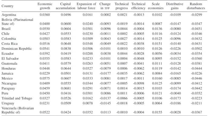
total factor productivity is broken down according to the model described in section IV. Table 3 shows the
country averages of the decomposition throughout the period analysed (1962-2010).1 The results shown in tables 3, 4, 5, 6, 7 and 8 are the average values for each country over 10-year time intervals.
The average economic growth rate in Latin America in the 50 years of the study was 4.2%, whereas the rate of change of tfp for the sample as a whole was -0.3% in that period (see table 3). The following tables present those rates separately for each country.
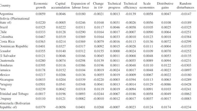
In general, the results agree with those obtained in the studies by de Fajnzylber, Loayza and Calderón (2002) on the growth of the Latin American economies and other countries. Tables 6 and 7 show that the economic growth rates of some countries in the 1990s were less than those recorded in the previous decade. A case in point is Colombia, which grew by 4.67% between 1981 and 1990, and by 4.55% in the following decade. Cárdenas (2007), who obtains similar results, also shows that the long-term economic growth rate in Colombia has fallen since 1980 owing to increasing levels of violence fuelled by an expansion in drug trafficking activities. Among other countries, the Bolivarian Republic of Venezuela recorded growth of 3.7% between 1980 and 1990, but only 3.6% in the following decade.
1 The breakdown was performed as from 1962 owing to the availability
TABLE 3
TFP results: averages 1962-2010
Country Economic growth
Capital accumulation
Expansion of labour force
Change in tfp
Technical progress
Technical efficiency
Scale economies
Distributive gains
Random disturbances
Argentina 0.0360 0.0496 0.0161 0.0002 0.0021 -0.0013 0.0102 -0.0109 -0.0299 Bolivia (Plurinational
State of) 0.0400 0.0600 0.0240 -0.0093 -0.0019 -0.0014 0.0087 -0.0147 -0.0347 Brazil 0.0550 0.0604 0.0301 0.0096 0.0044 -0.0004 0.0136 -0.0080 -0.0451 Chile 0.0427 0.0553 0.0230 -0.0011 0.0002 -0.0005 0.0116 -0.0124 -0.0346 Colombia 0.0503 0.0583 0.0309 0.0043 0.0027 -0.0014 0.0125 -0.0096 -0.0432 Costa Rica 0.0516 0.0648 0.0348 -0.0049 -0.0022 -0.0038 0.0151 -0.0140 -0.0431 Dominican Republic 0.0541 0.0838 0.0306 -0.0101 0.0010 -0.0010 0.0126 -0.0226 -0.0502 Ecuador 0.0392 0.0419 0.0288 0.0038 0.0044 -0.0028 0.0056 -0.0034 -0.0354 El Salvador 0.0355 0.0583 0.0233 -0.0101 0.0004 -0.0048 0.0095 -0.0152 -0.0360 Guatemala 0.0411 0.0579 0.0263 -0.0051 0.0007 -0.0041 0.0111 -0.0128 -0.0381 Honduras 0.0448 0.0644 0.0327 -0.0079 0.0006 -0.0062 0.0119 -0.0142 -0.0444 Jamaica 0.0229 0.0501 0.0131 -0.0177 -0.0035 -0.0062 0.0084 -0.0165 -0.0226 Mexico 0.0575 0.0607 0.0333 0.0081 0.0017 -0.0011 0.0160 -0.0085 -0.0446 Nicaragua 0.0409 0.0555 0.0344 -0.0077 -0.0005 -0.0098 0.0125 -0.0099 -0.0412 Paraguay 0.0459 0.0681 0.0291 -0.0071 0.0014 -0.0015 0.0103 -0.0174 -0.0442 Peru 0.0450 0.0416 0.0301 0.0086 0.0011 -0.0006 0.0121 -0.0040 -0.0352 Trinidad and Tobago 0.0327 0.0526 0.0162 -0.0137 -0.0066 -0.0005 0.0106 -0.0173 -0.0223 Uruguay 0.0231 0.0509 0.0078 -0.0145 -0.0018 -0.0005 0.0064 -0.0186 -0.0211 Venezuela (Bolivarian
Republic of) 0.0522 0.0424 0.0352 0.0113 -0.0010 -0.0004 0.0155 -0.0028 -0.0367
Source: prepared by the authors. tfp: total factor productivity.
TABLE 4
TFP decomposition: averages 1962-1970
Country Economic growth
Capital accumulation
Expansion of labour force
Change in tfp
Technical progress
Technical efficiency
Scale economies
Distributive gains
Random disturbances
Argentina 0.0802 0.1549 0.0143 -0.0438 -0.0183 -0.0006 0.0205 -0.0454 -0.0452 Bolivia (Plurinational
State of) 0.0681 0.1785 0.0182 -0.0717 -0.0174 -0.0012 0.0132 -0.0663 -0.0569 Brazil 0.1014 0.1568 0.0328 -0.0263 -0.0143 -0.0008 0.0215 -0.0328 -0.0619 Chile 0.0641 0.1421 0.0137 -0.0529 -0.0198 -0.0005 0.0161 -0.0487 -0.0388 Colombia 0.0771 0.1477 0.0242 -0.0438 -0.0165 -0.0005 0.0162 -0.0431 -0.0509 Costa Rica 0.0718 0.1599 0.0327 -0.0647 -0.0212 -0.0012 0.0172 -0.0596 -0.0560 Dominican Republic 0.0939 0.2030 0.0417 -0.0695 -0.0169 -0.0007 0.0168 -0.0688 -0.0813 Ecuador 0.0723 0.1450 0.0259 -0.0506 -0.0195 -0.0014 0.0177 -0.0474 -0.0481 El Salvador 0.0812 0.1701 0.0364 -0.0609 -0.0188 -0.0013 0.0174 -0.0581 -0.0644 Guatemala 0.0764 0.1709 0.0256 -0.0619 -0.0182 -0.0012 0.0165 -0.0590 -0.0582 Honduras 0.0759 0.1909 0.0310 -0.0775 -0.0185 -0.0029 0.0155 -0.0717 -0.0685 Jamaica 0.0579 0.1626 0.0114 -0.0745 -0.0227 -0.0008 0.0159 -0.0669 -0.0416 Mexico 0.1066 0.1802 0.0299 -0.0385 -0.0175 -0.0005 0.0263 -0.0468 -0.0650 Nicaragua 0.0826 0.2100 0.0321 -0.0854 -0.0203 -0.0005 0.0183 -0.0830 -0.0741 Paraguay 0.0608 0.1528 0.0260 -0.0640 -0.0163 -0.0007 0.0098 -0.0567 -0.0540 Peru 0.0781 0.1452 0.0235 -0.0440 -0.0195 -0.0005 0.0200 -0.0441 -0.0466 Trinidad and Tobago 0.0427 0.1243 0.0110 -0.0672 -0.0252 -0.0005 0.0125 -0.0540 -0.0254 Uruguay 0.0436 0.1174 0.0083 -0.0561 -0.0205 -0.0007 0.0108 -0.0458 -0.0260 Venezuela (Bolivarian
Republic of) 0.0853 0.1485 0.0304 -0.0430 -0.0212 -0.0004 0.0236 -0.0451 -0.0505
TABLE 5
TFP decomposition: averages 1971-1980
Country Economic growth
Capital accumulation
Expansion of labour force
Change in tfp
Technical progress
Technical efficiency
Scale economies
Distributive gains
Random disturbances
Argentina 0.0409 0.0608 0.0145 -0.0133 -0.0096 0.0001 0.0117 -0.0156 -0.0211 Bolivia (Plurinational
State of) 0.0375 0.0495 0.0228 -0.0108 -0.0081 0.0001 0.0084 -0.0112 -0.0240 Brazil 0.0810 0.1003 0.0359 -0.0026 -0.0059 0.0000 0.0208 -0.0176 -0.0525 Chile 0.0334 0.0192 0.0260 0.0020 -0.0098 0.0002 0.0089 0.0026 -0.0139 Colombia 0.0521 0.0612 0.0302 -0.0056 -0.0074 0.0001 0.0127 -0.0110 -0.0336 Costa Rica 0.0667 0.0837 0.0410 -0.0144 -0.0124 -0.0007 0.0185 -0.0198 -0.0436 Dominican Republic 0.0681 0.1119 0.0345 -0.0255 -0.0088 -0.0001 0.0161 -0.0327 -0.0528 Ecuador 0.0211 0.0353 0.0273 -0.0111 0.0125 -0.0091 -0.0196 0.0051 -0.0304 El Salvador 0.0462 0.0699 0.0299 -0.0194 -0.0098 -0.0049 0.0126 -0.0174 -0.0341 Guatemala 0.0479 0.0762 0.0227 -0.0192 -0.0097 0.0003 0.0122 -0.0220 -0.0318 Honduras 0.0418 0.0678 0.0230 -0.0201 -0.0098 0.0000 0.0101 -0.0203 -0.0289 Jamaica 0.0367 0.0339 0.0299 -0.0096 -0.0138 -0.0074 0.0133 -0.0017 -0.0175 Mexico 0.0781 0.0671 0.0505 0.0084 -0.0084 0.0001 0.0219 -0.0052 -0.0479 Nicaragua 0.0455 0.0459 0.0368 -0.0086 -0.0114 -0.0066 0.0135 -0.0042 -0.0286 Paraguay 0.0619 0.1194 0.0301 -0.0343 -0.0081 0.0006 0.0131 -0.0399 -0.0533 Peru 0.0402 0.0248 0.0312 0.0036 -0.0096 -0.0002 0.0111 0.0023 -0.0194 Trinidad and Tobago 0.0636 0.1078 0.0299 -0.0334 -0.0165 -0.0001 0.0207 -0.0375 -0.0406 Uruguay 0.0256 0.0734 0.0035 -0.0347 -0.0114 0.0002 0.0070 -0.0305 -0.0165 Venezuela (Bolivarian
Republic of) 0.0745 0.0644 0.0469 0.0040 -0.0121 0.0001 0.0228 -0.0067 -0.0409
Source: prepared by the authors. tfp: total factor productivity.
TABLE 6
TFP decomposition: averages 1981-1990
Country Economic growth
Capital accumulation
Expansion of labour force
Change in tfp
Technical progress
Technical efficiency
Scale economies
Distributive gains
Random disturbances
Argentina 0.0059 0.0046 0.0180 -0.0021 0.0013 -0.0139 0.0058 0.0047 -0.0147 Bolivia (Plurinational
State of) 0.0220 -0.0005 0.0246 0.0168 0.0031 -0.0026 0.0056 0.0108 -0.0189 Brazil 0.0325 0.0222 0.0311 0.0117 0.0046 -0.0058 0.0105 0.0025 -0.0325 Chile 0.0333 0.0128 0.0290 0.0164 0.0017 -0.0007 0.0090 0.0064 -0.0251 Colombia 0.0467 0.0319 0.0369 0.0164 0.0033 -0.0010 0.0123 0.0018 -0.0384 Costa Rica 0.0363 0.0214 0.0369 0.0079 -0.0016 -0.0113 0.0136 0.0072 -0.0299 Dominican Republic 0.0401 0.0327 0.0317 0.0092 0.0015 -0.0028 0.0111 -0.0004 -0.0335 Ecuador 0.0355 0.0140 0.0312 0.0155 0.0000 -0.0024 0.0109 0.0070 -0.0252 El Salvador 0.0121 0.0046 0.0166 0.0045 0.0011 -0.0068 0.0048 0.0053 -0.0135 Guatemala 0.0280 0.0074 0.0298 0.0139 0.0011 -0.0055 0.0089 0.0094 -0.0231 Honduras 0.0395 0.0116 0.0386 0.0196 0.0011 -0.0048 0.0110 0.0122 -0.0303 Jamaica 0.0178 0.0152 0.0104 0.0019 -0.0024 0.0017 0.0048 -0.0023 -0.0097 Mexico 0.0217 0.0206 0.0136 0.0055 0.0019 -0.0009 0.0067 -0.0022 -0.0180 Nicaragua 0.0033 0.0204 0.0339 -0.0220 -0.0003 -0.0394 0.0113 0.0063 -0.0289 Paraguay 0.0501 0.0541 0.0348 0.0041 0.0013 -0.0014 0.0129 -0.0086 -0.0428 Peru 0.0239 0.0042 0.0318 0.0119 0.0019 -0.0094 0.0091 0.0103 -0.0241 Trinidad and Tobago -0.0017 0.0196 0.0093 -0.0244 -0.0067 -0.0186 0.0058 -0.0049 -0.0062 Uruguay 0.0110 0.0121 0.0082 -0.0010 -0.0012 -0.0017 0.0037 -0.0017 -0.0083 Venezuela (Bolivarian
Republic of) 0.0379 -0.0056 0.0401 0.0268 -0.0007 -0.0023 0.0124 0.0174 -0.0234
TABLE 7
TFP decomposition: averages 1991-2000
Country Economic growth
Capital accumulation
Expansion of labour force
Change in tfp
Technical progress
Technical efficiency
Scale economies
Distributive gains
Random disturbances
Argentina 0.0327 0.0128 0.0144 0.0322 0.0129 0.0131 0.0057 0.0006 -0.0267 Bolivia (Plurinational
State of) 0.0323 0.0124 0.0305 0.0285 0.0149 -0.0018 0.0075 0.0079 -0.0391 Brazil 0.0344 0.0124 0.0292 0.0322 0.0161 0.0028 0.0086 0.0047 -0.0395 Chile 0.0372 0.0532 0.0184 0.0087 0.0125 0.0001 0.0102 -0.0140 -0.0431 Colombia 0.0455 0.0263 0.0406 0.0287 0.0145 -0.0039 0.0130 0.0051 -0.0501 Costa Rica 0.0460 0.0235 0.0335 0.0287 0.0097 0.0015 0.0129 0.0046 -0.0397 Dominican Republic 0.0357 0.0407 0.0218 0.0140 0.0124 0.0004 0.0093 -0.0082 -0.0408 Ecuador 0.0327 -0.0001 0.0338 0.0328 0.0118 -0.0030 0.0100 0.0139 -0.0337 El Salvador 0.0316 0.0255 0.0188 0.0209 0.0125 0.0047 0.0068 -0.0031 -0.0336 Guatemala 0.0247 0.0166 0.0217 0.0190 0.0127 -0.0031 0.0073 0.0021 -0.0326 Honduras 0.0418 0.0336 0.0441 0.0170 0.0125 -0.0145 0.0142 0.0048 -0.0530 Jamaica 0.0065 0.0259 0.0069 -0.0043 0.0085 -0.0084 0.0045 -0.0089 -0.0220 Mexico 0.0562 0.0194 0.0503 0.0398 0.0138 -0.0003 0.0165 0.0098 -0.0533 Nicaragua 0.0515 -0.0018 0.0397 0.0507 0.0119 0.0084 0.0111 0.0194 -0.0371 Paraguay 0.0297 0.0181 0.0267 0.0210 0.0123 -0.0039 0.0086 0.0039 -0.0360 Peru 0.0480 0.0101 0.0376 0.0421 0.0138 0.0071 0.0109 0.0103 -0.0418 Trinidad and Tobago 0.0331 -0.0066 0.0188 0.0360 0.0052 0.0107 0.0075 0.0126 -0.0150 Uruguay 0.0205 0.0300 0.0104 0.0072 0.0099 0.0008 0.0057 -0.0091 -0.0271 Venezuela (Bolivarian
Republic of) 0.0369 -0.0047 0.0361 0.0388 0.0116 0.0010 0.0107 0.0156 -0.0334
Source: prepared by the authors. tfp: total factor productivity.
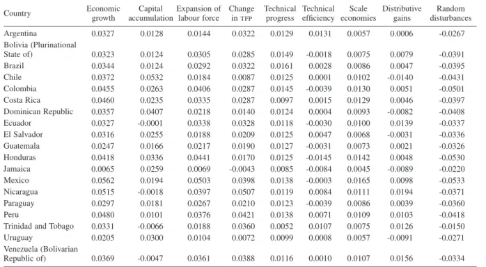
TABLE 8
TFP decomposition: averages 2001-2010
Country Economic growth
Capital accumulation
Expansion of labour force
Change in tfp
Technical progress
Technical efficiency
Scale economies
Distributive gains
Random disturbances
Argentina 0.0201 0.0150 0.0192 0.0279 0.0243 -0.0050 0.0072 0.0014 -0.0420 Bolivia (Plurinational
State of) 0.0254 0.0063 0.0281 0.0380 0.0265 -0.0047 0.0065 0.0096 -0.0471 Brazil 0.0257 0.0101 0.0217 0.0328 0.0213 0.0017 0.0065 0.0033 -0.0390 Chile 0.0455 0.0492 0.0279 0.0204 0.0166 -0.0015 0.0138 -0.0085 -0.0520 Colombia 0.0300 0.0246 0.0229 0.0257 0.0196 -0.0019 0.0085 -0.0006 -0.0431 Costa Rica 0.0370 0.0354 0.0300 0.0179 0.0145 -0.0073 0.0131 -0.0024 -0.0464 Dominican Republic 0.0326 0.0306 0.0233 0.0213 0.0168 -0.0019 0.0096 -0.0031 -0.0426 Ecuador 0.0342 0.0152 0.0261 0.0326 0.0174 0.0017 0.0091 0.0044 -0.0396 El Salvador 0.0062 0.0212 0.0150 0.0043 0.0171 -0.0157 0.0058 -0.0028 -0.0343 Guatemala 0.0282 0.0184 0.0317 0.0228 0.0177 -0.0108 0.0104 0.0055 -0.0448 Honduras 0.0250 0.0179 0.0268 0.0214 0.0175 -0.0087 0.0088 0.0039 -0.0412 Jamaica -0.0045 0.0127 0.0070 -0.0019 0.0132 -0.0160 0.0036 -0.0027 -0.0222 Mexico 0.0248 0.0164 0.0220 0.0252 0.0187 -0.0038 0.0085 0.0017 -0.0387 Nicaragua 0.0216 0.0030 0.0293 0.0268 0.0174 -0.0110 0.0082 0.0121 -0.0375 Paraguay 0.0268 -0.0041 0.0281 0.0375 0.0179 -0.0020 0.0073 0.0144 -0.0347 Peru 0.0347 0.0235 0.0262 0.0293 0.0191 -0.0002 0.0094 0.0011 -0.0443 Trinidad and Tobago 0.0258 0.0178 0.0122 0.0202 0.0103 0.0061 0.0066 -0.0028 -0.0244 Uruguay 0.0147 0.0218 0.0085 0.0120 0.0145 -0.0010 0.0046 -0.0061 -0.0277 Venezuela (Bolivarian
Republic of) 0.0266 0.0094 0.0226 0.0298 0.0172 -0.0004 0.0079 0.0050 -0.0352
Table 3 also shows that the countries that recorded a larger contribution of technical progress to productivity growth in the 50-year period analysed were Argentina, Brazil, Colombia and Ecuador, with indices of around 0.3%. Brazil displayed an average index of 0.4%, as well as the highest indices in the last three decades (see tables 6, 7 and 8). These results coincide with those reported by Pires and Garcia (2004), which also identified low rates of technical progress in Brazil between 1970 and 2000, because the authors take account of the fact that this country was not a member of the Organisation for Economic Co-operation and Development (oecd), and that the markets of the Bolivarian Republic of Venezuela, Mexico and Peru underwent a process of import substitution related to episodes of economic liberalization, during which the industrialization process slowed down.
As shown in table 3, the 19 countries analysed in this study recorded decreasing technical efficiency, which assumes that the contribution of that efficiency to tfp was negative in all countries. Nonetheless, there was some technical progress in most cases, and output increased in all of them. It is well known that technical efficiency is determined by the distance from the technological frontier and effective use of technologies, so these results suggest that the expansion of the frontier was more intense and faster than the dissemination of new technologies. In other words, some of the countries analysed did not fully keep pace with the technological developments that occurred in the period analysed, possibly owing to problems in the process of diffusion and adoption of more modern technologies.
In a general analysis of the decomposition of tfp, table 8 shows that most of the countries display positive allocative gains, including Brazil. Those results reflect improvements in resource allocation among the factors of production used in those countries.
These results agree with those reported by Pires and Garcia (2004), whose estimations show that Costa Rica and Trinidad and Tobago displayed the largest distributive gains, represented by indices of 4.2% and 13.5%, respectively. Those two countries were also the leaders in the sample in terms of technical progress during the period studied.
Tables 4 and 5 show that Brazil suffered allocative efficiency losses in the first two decades analysed, which are the clear result of a growth strategy that did not take account of the adjustment. It can also be seen that both output and physical capital grew more strongly in the 1970s than in other decades. Those findings agree with those obtained by Pires and Garcia (2004), who argue that in the 1970s there was an intensive process of resource allocation in the economy, which led to a considerable investment in infrastructure in Brazil.
The analysis of the data presented in tables 4 and 5 shows that the indices of economic growth in Brazil were higher in the first two decades before dropping to around 3% between 1980 and 2000. This is explained by a slackening of growth in the country owing to the exhaustion of the industrialization-via-import-substitution model.
In the five decades examined separately, only Trinidad and Tobago posted negative growth in the decade 1981-1990. In general, the pattern of economic growth in the countries is similar, and, as shown in table 6, the average does not exceed 6% in the period studied. The cases of Brazil, Colombia and Paraguay stand out as those with the highest indices of economic growth, averaging 4.3%. The countries with the lowest average growth indices were Argentina and Uruguay, with just 0.59% and 1.10%, respectively.
As can be seen in table 4, all of the Latin American countries analysed displayed negative indices of tfp variation in the first period studied (1962-1970). This situation changed in the subsequent decades, when some countries displayed positive indices. Table 7 and 8 show that all countries except the Jamaica achieved positive indices of tfp growth in the decades of 1990 and 2000. The average growth rate of Brazilian productivity throughout the period analysed were 0.9% per year (see table 3).
VI
Final thoughts
The analysis of tfp and its components in Latin America in the period 1960-2010, using a stochastic-frontier model which includes macroeconomic variables of technical inefficiency, shows that those variables generally have a significant effect that enables better understanding of technical inefficiency throughout the region.
The significance of the effects is found both through likelihood tests and through the parameter g, of value 0.51, in the model estimation.
The most important variables for explaining the technical inefficiency of the sample countries, in other words those that display a positive relation to inefficiency, are public expenditure and the inflation rate: the higher these rates are, the more they are associated with technical inefficiency.
In contrast, the variable corresponding to the deviation of local prices from purchasing power parity (used as a proxy variable for the exchange rate) displays an inverse relation with respect to technical inefficiency: the larger deviation of this relative price, the less is technical inefficiency.
Although relatively low throughout the period studied, the average rate of economic growth of the
countries studied was positive. Brazil is one of the leading countries in this respect, with a growth rate of 5.5%. The analysis of the 1960s and 1970s shows that the average Brazilian growth rates were around 7%, which possibly coincides with the adoption of the import substitution industrialization model in the countries of the region.
Costa Rica, the Dominican Republic, Ecuador, Guatemala, Mexico and Paraguay recorded similar average gdp growth rates of 5.1%; 4.0%; 4.1%; 5.7%; 4.5%, and 5.4%, respectively. The worst performer in the period was Uruguay, where the average growth rate was just 2.3%.
The results of the decomposition of the change in tfp into technical progress, technical efficiency, economies of scale and distributive gains vary between the countries analysed. Although there is unanimity with respect to technical progress (the average was positive in most of the countries throughout the period analysed), the results in terms of the other components are different.
Lastly, it is worth stressing that the great advantage of this tfp decomposition model compared to that known as the Malmquist index is the possibility of incorporating scale and allocative effects in the analysis of the results.
Bibliography
Aigner, D.J., C.A.K. Lovell and P. Schmidt (1977), “Formulation and estimation of stochastic frontier production functions models”, Journal of Econometrics, vol. 6, No. 1, Amsterdam, Elsevier. Battese, G.E. and T.J. Coelli (1995), “A model for technical inefficiency effects in stochastic frontier production functions for panel data”, Empirical Economics, vol. 20, No. 2, Springer. (1993), “A stochastic frontier production incorporating a model for technical inefficiency effects”, Working Papers in Econometrics and Applied Statistics, No. 69, Armidale, University of New England.
Battese, G.E. and G.S. Corra (1977), “Estimation of a production frontier model: with application to the pastoral zone of eastern Australia”, Australian Journal of Agricultural Economics, vol. 21, No. 3, Canberra, Australian Agricultural and Resource Economics Society.
Bauer, P.W. (1990), “Recent developments in the econometric estimation of frontiers”, Journal of Econometrics, vol. 46, No. 1-2, Amsterdam, Elsevier.
Bittencourt, A. and Marinho, E. (2007), “Produtividade e crescimento econômico na América Latina: a abordagem da fronteira de produção estocástica”, Estudos Econômicos, vol. 37, No. 1, São Paulo, Instituto de Pesquisas Econômicas.
Cárdenas, M. (2007), “Economic growth in Colombia: a reversal of fortune?”, Ensayos sobre Política Económica, vol. 25, No. 53, Bogota, Bank of the Republic.
Coelli, T.J., D.S.P. Rao and G.E. Battese (1998), An Introduction to Efficiency and Productivity Analysis, Kluwer Academic Publishers.
De Gregorio, J. (1992), “Economic growth in Latin America”, Journal of Development Economics, vol. 39, No. 1, Amsterdam, Elsevier. Fajnzylber, P., N. Loayza and C. Calderón (2002), Economic Growth in Latin America and the Caribbean: Stylized Facts, Explanation and Forecasts, Washington, D.C., World Bank. Färe, R. and others (1994), “Productivity growth, technical progress,
and efficiency change in industrialized countries”, American Economic Review, vol. 84, No. 1, Nashville, Tennessee, American Economic Association.
(1992), “Productivity changes in Swedish pharmacies 1980-1989: a non-parametric Malmquist approach”, Journal of Productivity Analysis, vol. 3, No. 1-2, Springer.
Färe, R., S. Grosskopf and P. Roos (1998), “Malmquist productivity indexes: a survey of theory and practice”, Index Numbers: Essays in Honour of Sten Malmquist, Kluwer Academic Publishers. Griliches, Z. (1996), “The discovery of the residual: a historical note”,
Journal of Economic Literature, vol. 34, No. 3, Nashville, Tennessee, American Economic Association.
Johnson, A.L. and T. Kuosmanen (2012), “One-stage and two-stage dea estimation of the effects of contextual variable”, European Journal of Operational Research, vol. 220, No. 2, Amsterdam, Elsevier.
Klein, P.G. and H. Luu (2001), Politics and Productivity, Merril Lynch Capital Markets Bank Ltd.
Kodde, D.A. and F.C. Palm (1986), “Wald criteria for jointly testing equality and inequality restrictions”, Econometrica, vol. 54, No. 5, New York, The Econometric Society.
Kumbhakar, S.C. (2000), “Estimation and decomposition of productivity change when production is not efficient”, Econometric Reviews, vol. 19, No. 4, Taylor & Francis. Kumbhakar, S.C. and C.A.K. Lovell (2003), Stochastic Frontier
Analysis, New York, Cambridge University Press.
Laborda, L., D. Sotelsek and J.L. Guasch (2011), “Innovative and absorptive capacity of international knowledge: an empirical analysis of productivity sources in Latin American countries”, Latin American Business Review, vol. 12, No. 4, Taylor & Francis.
Lee, C.Y. and others (2013), “A more efficient algorithm for convex nonparametric least squares”, European Journal of Operational Research, vol. 227, No. 2, Amsterdam, Elsevier.
Maudos, J., J.M. Pastor and L. Serrano (1999), “Total factor productivity measurement and human capital in oecd countries”, Economics Letters, vol. 63, No. 1, Amsterdam, Elsevier.
Meeusen, W. and V.D. Broeck (1977), “Efficiency estimation from Cobb-Douglas production functions with composed error”, International Economic Review, vol. 18, No. 2, Wiley. Orea, L. (2002), “Parametric decomposition of a generalized
Malmquist productivity index”, Journal of Productivity Analysis, vol. 18, No. 1, Kluwer Academic Publishers. Pires, J.O. and F. Garcia (2004), “Productivity of nations: a stochastic
frontier approach to tfp decomposition”, Econometric Society Latin American Meetings, No. 292, Econometric Society. Pitt, M.M. and L.F. Lee (1981), “The measurement and sources
of technical inefficiency in the Indonesian weaving industry”, Journal of Development Economics, vol. 9, No. 1, Amsterdam, Elsevier.
Sauer, J., K. Frohberg and H. Hockmann (2006), “Stochastic efficiency measurement: the curse of theoretical consistency”, Journal of Applied Economics, vol. 9, No. 1, cema University. Schmidt, P. and R. Sickles (1984), “Production frontiers and panel data”, Journal of Business and Economic Statistics, vol. 2, No. 4, Taylor & Francis.
Solow, R.M. (1957), “Technical change and the aggregate production function”, Review of Economic and Statistics, vol. 39, No. 3, Cambridge, Massachusetts, The mit Press.