Analytical methods to study fate of organic pollutants in environment

(1)

DIANA LUÍSA

DUARTE DE LIMA

MÉTODOS ANALÍTICOS: DESTINO AMBIENTAL DE

POLUENTES ORGÂNICOS

ANALYTICAL METHODS TO STUDY FATE OF

ORGANIC POLLUTANTS IN ENVIRONMENT

(2)

DIANA LUÍSA

DUARTE DE LIMA

MÉTODOS ANALÍTICOS: DESTINO AMBIENTAL DE

POLUENTES ORGÂNICOS

ANALYTICAL METHODS TO STUDY FATE OF

ORGANIC POLLUTANTS IN ENVIRONMENT

Tese apresentada à Universidade de Aveiro para cumprimento dos requisitos necessários à obtenção do grau de Doutor em Química, realizada sob a orientação científica do Doutor Valdemar Inocêncio Esteves, Professor Auxiliar do Departamento de Química da Universidade de Aveiro e do Doutor Rudolf Josef Schneider, Investigador com agregação do BAM Federal Institute for Materials and Testing e lecturer da Technical University of Berlin.

Apoio financeiro da FCT e do FSE no âmbito do QREN-POPH.Tipologia 4.1 Apoio via Bolsa de Doutoramento SFRH/BD/36086/2007.

(3)

(4)

o júri

presidente Prof. Doutor Aníbal Manuel de Oliveira Duarte

professor catedrático da Universidade de Aveiro

Prof. Doutor Rudolf Josef Schneider

Investigador com agregação do BAM Federal Institute for Materials Research and Testing e

lecturer da Technical University of Berlin, Germany

Prof. Doutor Joaquim Esteves da Silva

professor associado com agregação da Faculdade de Ciências da Universidade do Porto

Prof. Doutora Marcela Alves Segundo

professora auxiliar da Faculdade de Farmácia da Universidade do Porto

Prof. Doutora Maria Eduarda Bastos Henriques dos Santos professora auxiliar da Universidade de Aveiro

Prof. Doutor Valdemar Inocêncio Esteves professor auxiliar da Universidade de Aveiro

(5)

agradecimentos A realização e conclusão deste trabalho não teria sido possível sem a colaboração, presença e apoio de diversas pessoas a quem eu gostaria de deixar expresso o meu reconhecimento e profundo agradecimento.

Ao meu orientador, Doutor Valdemar I. Esteves, por toda a amizade, apoio, paciência e motivação que sempre me transmitiu, quer nos bons momentos, quer nos menos bons, e que me fizeram olhar em frente e nunca desistir!

Ao meu co-orientador, Rudolf J. Schneider, pela sua inteira disponibilidade e apoio durante a realização deste trabalho. À BAM Federal Institute for Materials and Testing por me ter proporcionado as condições necessárias à realização de um estágio sobre ensaios imunológicos nas suas instalações. Ao INRES – Institute of Plant Nutrition, University of Bonn pelas amostras de solos disponibilizadas para a realização deste trabalho.

À Escola Superior de Tecnologia da Saúde de Coimbra, sua Direcção, corpo docente e funcionários, pela compreensão e flexibilidade de horário ao longo destes quatro anos. Um agradecimento especial à Paula Fonseca, pela amizade, apoio e incentivo.

Aos meu colegas de trabalho e amigos, em particular à Pati, à Luci e à DiMoni, por toda a amizade, pelos bons momentos de convívio e, principalmente, pela alegria que trazem à minha vida.

Ao grupo de Química Analítica e Ambiental pelo seu companheirismo, em particular à Patrícia Silva, à Vânia Calisto, ao Guillaume Erny e à Joana Leal pela sua colaboração em algumas partes deste trabalho.

Aos amigos de sempre, Isaura, Micas, Cátia, Paulinha e Carlos, simplesmente por fazerem parte da minha vida.

Aos meus amigos e familiares, em particular, ao meu pai e irmão pela amizade, compreensão e motivação.

À minha mãe, por tudo o que me proporcionou ao longo da vida, pelo exemplo de Mulher de força e coragem que é, e pelo facto de que, sem ela, nunca poderia ser quem sou.

As palavras finais vão para o meu chatinho, por me fazer sorrir sempre que tinha vontade de chorar!

(6)

palavras-chave Atrazina, 17α-etinilestradiol, adsorção-dessorção, electroforese capilar, desconvolução espectral, ELISA.

resumo O transporte de poluentes no ambiente envolve processos distintos, tais como

a volatilização, a lixiviação e escoamento através dos solos atingindo águas superficiais. A adsorção e a dessorção são dos factores que mais influenciam a lixiviação, tendo assim um papel fundamental no destino dos poluentes orgânicos e na sua distribuição no sistema solo/água. O trabalho desenvolvido envolve a optimização de metodologias analíticas para a monitorização da sorção de poluentes orgânicos, 17α-etinilestradiol (EE2) e atrazina, e do seu destino no ambiente aquático.

Inicialmente, foram desenvolvidas várias metodologias, baseadas na cromatografia micelar electrocinética, na desconvolução de espectros de absorvência e de fluorescência, e, ainda, em ensaios imunoenzimáticos. Neste trabalho, encontram-se também descritas as optimizações dos referidos métodos juntamente com a avaliação do seu desempenho. Avaliou-se ainda a aplicabilidade dos métodos desenvolvidos fazendo estudos de adsorção da atrazina e do EE2, a diferentes amostras de solos. O trabalho desenvolvido faculta assim várias opções, no que diz respeito a metodologias analíticas para monitorizar a adsorção da atrazina a solos, incrementado a liberdade de escolha, a qual será dependente das condições disponíveis no laboratório e das preferências do analista.

Na segunda parte do trabalho faz-se o estudo do comportamento de sorção dos dois poluentes orgânicos em causa a diferentes amostras de solos. A caracterização química da matéria orgânica dos solos serve de base para a interpretação dos mecanismos de interacção responsáveis pelas ligações estabelecidas entre os poluentes e os constituintes do solo. No caso da atrazina, os resultados demonstraram que os grupos aromáticos e carboxílicos da matéria orgânica dos solos são os agentes de ligação mais eficientes. O EE2 liga-se fortemente à matéria orgânica e é essencialmente estabilizado por interacções hidrofóbicas através de associações face-a-face dos núcleos aromáticos do EE2 com os da superfície dos solos e/ou com os das outras moléculas de EE2. A fertilização com estrumes de animais introduz mais estruturas aromáticas e grupos carboxílicos, indicando que a sua utilização poderá minimizar a toxicidade residual do EE2 e da atrazina presente nos solos, através do aumento da sua adsorção e, consequentemente, redução da sua lixiviação.

Uma vez que as águas residuais, superficiais e/ou subterrâneas podem ser o destino final dos poluentes orgânicos, foi ainda realizada a quantificação do EE2 e da atrazina em diversas amostras de diferentes ambientes aquáticos.

(7)

keywords Atrazine, 17α-ethinylestradiol, adsorption-desorption, capillary electrophoresis, spectral deconvolution, ELISA.

abstract Environmental transport of pollutants comprises distinct processes such as

volatilization, leaching and surface runoff. Sorption is one of the most important phenomena that affects leaching, and thus the fate of hydrophobic organic pollutants in soils and also control their distribution in the soil/water environment. The work developed focuses the optimization of analytical techniques for monitoring the sorption behaviour of organic pollutants, 17α-ethinylestradiol (EE2) and atrazine, and their fate in aqueous environment. Initially, the development of several analytical techniques, such as micellar electrokinetic chromatography, spectral deconvolution, using UV-Vis and fluorescence spectroscopy, and also enzyme linked immunosorbent assay was performed. Optimization, method performance and recovery tests are

described and results discussed. Moreover, in order to evaluate the

applicability of the previously optimized method, atrazine and EE2 sorption to soil samples was performed. The work developed provide several options, in terms of methodology to follow sorption of atrazine onto soils, however the choice depends on the laboratory conditions and on the analyst preferences. The advantages and disadvantages of each methodology should be evaluated first.

The second part of this work consisted in the sorption behaviour study of those two different hydrophobic organic pollutants onto different soil samples. Soil organic matter chemical characterization, being essential to understand the binding mechanism responsible for the interactions, was made. The results of atrazine binding to organic matter pointed out that carboxyl units and aromatic-rich organic matter are the most efficient binding agents for atrazine. EE2 adsorbs strongly to soil organic matter and is mainly stabilized by hydrophobic interactions, through aromatic nuclei face to face with surface and/or another EE2 molecule association. Farmyard manure soil contains higher aromatic and carboxyl units, indicating that this type of manure can be effectively used to minimize the residual toxicity of EE2 and atrazine present in soils, increasing the sorption and reducing leaching onto water resources.

Since the final destination of organic pollutants can be ground, surface and/or waste water, atrazine and 17α-ethinylestradiol were quantified in several water samples.

(8)

(9)

PART I – Introduction Introduction

Hydrophobic organic pollutants ... 1

Atrazine ... 1

Description ... 1

Sources of pesticides in water... 2

17α-Ethinylestradiol ... 4

Description ... 4

Sources of estrogens in waters ... 5

Fate of HOP in the environment... 6

References ... 11

PART II – Development of analytical procedures to follow sorption behaviour of HOP onto soils Chapter 1 – Atrazine analysis by capillary electrophoresis 1.1. Introduction ... 15

1.2. Experimental procedure ... 16

1.2.1. Soil sample ... 16

1.2.2. Instrumentation ... 17

1.2.3. Buffer and standards ... 18

1.2.4. Capillary column conditioning ... 18

1.2.5. Separation conditions ... 19

1.2.6. Suitability of the MEKC method... 19

1.2.7. Adsorption studies ... 19

1.2.8. Data analysis ... 20

1.3. Results and discussion ... 21

1.3.1. Electrophoretic separation of atrazine ... 21

1.3.2. Performance of the method ... 22

1.3.3. Preliminary studies and kinetic experiments ... 23

1.3.4. Adsorption studies ... 24

1.3.5. MEKC and HPLC methods – comparison ... 26

1.4. Conclusions ... 28

1.5. References ... 29

Chapter 2 – Spectral deconvolution to follow sorption behaviour of organic pollutants 2.1. Introduction ... 31

(10)

2.3.1.1. Soil sample ... 34

2.3.1.2. Instrumentation ... 34

2.3.1.3. Adsorption studies ... 34

2.3.1.4. MEKC analysis ... 35

2.3.1.5. UV determination ... 35

2.3.2. Results and discussion ... 36

2.3.2.1. UV Spectral deconvolution method ... 36

2.3.2.2. Analytical curves by UVSD and MEKC... 37

2.3.2.3. Adsorption experiments – Evaluation of the analytical methods ... 38

2.4. Fluorescence SD for EE2 ... 40

2.4.1. Experimental procedure ... 40

2.4.1.1. Soil sample ... 40

2.4.1.2. Instrumentation ... 40

2.4.1.3. Fluorescence spectra acquisition ... 41

2.4.2.1. Fluorescence spectral deconvolution method ... 43

2.4.2.2. Evaluation of the deconvolution method... 45

2.4.2.3. Adsorption experiments ... 46

Chapter 3 – Development of an enzyme linked immunosorbent assay to follow atrazine sorption onto soils 3.1. Introduction ... 55

3.1.1. Antibodies ... 56

3.1.1.1. Structural and functional properties ... 57

3.1.1.2. Antibody production ... 58

3.1.2. Tracer synthesis ... 60

3.1.3. Immunoassays ... 62

3.1.4. Application in environmental analysis ... 66

3.1.4.1. Using ELISA to follow sorption behaviour ... 67

3.2.1. Soil sample ... 69

3.2.2. ELISA development ... 69

3.2.2.1. Reagents and materials ... 69

(11)

3.2.2.5. ELISA procedure... 78

3.2.3. Adsorption experiment ... 79

3.3.1. Tracer and antibody binding specificity ... 79

3.3.2. Optimization of antibody and tracer dilutions ... 88

3.3.3. Evaluation of assay performance ... 89

3.3.4. Evaluation of soil matrix effects ... 93

3.3.5 Adsorption experiment ... 95

PART III – Fate and persistence of HOP on environment Chapter 4 – Characterization of soil samples subjected to different organic long-term amendments 4.1. Introduction ... 101

4.2.1. Soil samples description ... 102

4.2.2. Total organic matter, total organic carbon, total nitrogen ... 102

4.2.3. 13C NMR spectroscopy ... 102

4.2.4. FT-IR spectroscopy ... 103

4.2.5. Capillary zone electrophoresis ... 103

4.3.1. Total organic matter, total organic carbon, total nitrogen ... 105

4.3.2. 13C NMR spectroscopy ... 106

4.3.3. FT-IR spectroscopy ... 108

4.3.4. Phenolic compounds content ... 111

Chapter 5 – Sorption behaviour of HOP on soils subjected to different organic long-term amendments 5.1. Introduction ... 119

5.2. Atrazine sorption behaviour ... 122

5.2.1.1. Soil samples ... 122

5.2.1.2. Instrumentation and analysis conditions ... 122

(12)

5.2.1.1. Adsorption ... 124

5.2.1.2 Desorption ... 127

5.3. EE2 sorption behaviour ... 132

5.3.1.1. Soil samples ... 132

5.3.1.2. Instrumentation and analysis conditions ... 132

5.3.1.4. Molecular modelling studies ... 132

Chapter 6 – Determination of HOP in water samples using ELISA 6.1. Introduction ... 149

6.2.1. Water samples ... 152

6.2.2. Reagents and materials ... 155

6.2.3. ELISA procedure ... 156

6.2.4. Matrix effects ... 157

6.3.1. Atrazine determination... 157

6.3.1.1. Evaluation of matrix effects... 157

6.3.1.2. Quantification of atrazine in ground, surface and wastewaters ... 165

6.3.2. EE2 determination ... 166

6.3.2.1. Optimization of antibody and tracer dilutions ... 166

6.3.2.2. Evaluation of assay performance ... 167

6.3.2.3. Cross-reactivity ... 169

6.3.2.4. Evaluation of matrix effects... 170

6.3.2.5. Quantification of EE2 in ground, surface and wastewaters ... 176

PART IV – Conclusions and Future work Conclusions ... 181

(13)

List of Figures

Figure I.I. Major pathways for pesticide transport into waters (Gerecke et al., 2002)…………3 Figure I.II. Pathways of pollutants degradation and transport……….…………...7 Figure 1.1. Chromatogram of an aqueous soil solution from a batch experimental sample (a)

matrix peak; (b) atrazine (c) ethylvanillin analysed using buffers with 0, 25 and 50 mmol L-1 SDS……….22

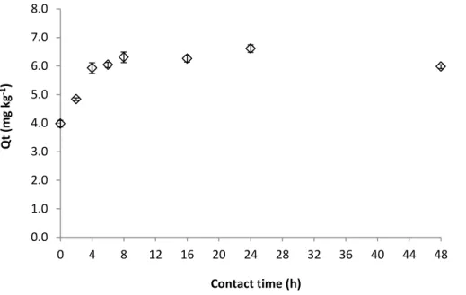
Figure 1.2. Influence of contact time on atrazine adsorption on soil. Initial atrazine

concentration 5 mg L-1 in 0.01 mol L-1 CaCl2 (n = 3); Qt – adsorbed concentration at time t

(h) (mg kg-1)……….………23

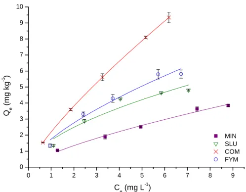
Figure 1.3. Freundlich adsorption isotherms for atrazine in soils subjected to different

fertilizations (MIN – mineral fertilizer; COM – compost fertilizer; FYM – farmyard manure; SLU – sewage sludge fertilizer; Error bars represent 95% confidence interval for n = 3)…….25

Figure 2.1. UV spectra from adsorption experiments on soil fertilized with sewage sludge (a)

UV Reference spectra of background (0.01 mol L-1 CaCl2), RSWE and atrazine; (b) Combined

spectrum of the three reference spectra; (c) Residual plots………37

Figure 2.2. Adsorption isotherms of atrazine onto soil fertilized with sewage sludge

obtained by UVSD (■) and by MEKC (x)……….……….39

Figure 2.3. Change in EE2 adsorption percentage with the soil/solution ratio; Initial EE2

concentration 2 mg L-1. Soil sample fertilized with farmyard manure………..…42

Figure 2.4. Residual plots obtained after the deconvolution of a 20 µg L-1 EE2 standard spiked into a farmyard manure soil extract using emission spectra range between a) 290 and 650 nm; b) 295 and 350 nm. λexc = 280 nm……….44

Figure 2.5. Influence of contact time on EE2 adsorption onto soil. Initial EE2 concentration

of 2 mg L-1 in 0.01 mol L-1 CaCl2 (n=3); Qt – adsorbed concentration at time t (h) (mg kg-1)……….47

(14)

Figure 2.6. Adsorption isotherms with fitting using Hill Equation; SLU, sewage sludge

fertilizer; MIN, mineral fertilizer; FYM, farmyard manure; COM, compost from organic

household waste; COM_LOI, composted soil submitted to loss on ignition……….…..………….48

Figure 3.1. Structural diagram representing the IgG (antibody); Fab = fragment of antigen binding region; Fc = constant fragment which binds to various cell receptors and complement proteins.……….57

Figure 3.2. The generation of hybridoma cells for monoclonal antibody production (adapted from Mikkelsen and Cortón, 2004)……….59

Figure 3.3. Coupling of the hapten to HRP using the mixed anhydride method………...61

Figure 3.4. Coupling of the hapten to HRP using the active ester method………62

Figure 3.5. Principle of non-competitive immunoassay – sandwich assay……….…63

Figure 3.6. Principle of direct competitive immunoassay……….………….…63

Figure 3.7. Principle of indirect competitive immunoassay………..64

Figure 3.8. Typical 4-parameter logistic function graph for a competitive immunoassay format……….…64

Figure 3.9. Triazine derivatives: a) 2-(tert-butylamino)-4-[(1-carboxypent-5-yl)amino]-6-(ethylamino)-1,3,5-triazine (t-Bu/Et/C6); b) 2-(tert-butylamino)-4-[(1-carboxyeth-2-yl-)thio]-6-(ethylamino)-1,3,5-triazine (t-Bu/Et/SC3); c) 2-[(1-carboxyeth-2-yl-)thio]-4-(ethylamino)-6-(isopropylamino)-1,3,5-triazine (i-Pr/Et/SC3); d) 2-[(1-carboxypent-5-yl)amino]-4-chloro-6-amino-1,3,5-triazine (H/Cl/C6); e) 2-(tert-butylamino)-4-[(1-carboxypent-5-yl)amino]-6-chloro-1,3,5-triazine (t-bu/Cl/C6); f) 2-[(1-carboxypent-5-yl)amino]-4-(ethylamino)-6-(isopropylamino)-1,3,5-triazine (i-Pr/Et/C6); g) 2-[(1-carboxypent-5-yl)amino]-4-chloro-6-(isopropylamino)-1,3,5-triazine (i-Pr/Cl/C6); (for nomenclature and abbreviations, cf. to Weller and Niessner, 1997)……………70

Figure 3.10. Collection of the tracer T1: t-Bu/Et/C6 fractions after separation by means of a Sephadex G-25 PD-10® column using mixed anhydride method………72

Figure 3.11. Collection of the tracer T2: t-Bu/Et/SC3 fractions after separation by means of a Sephadex PD-10® column using mixed anhydride method………73

Figure 3.12. Collection of the tracer T3: Et/i-Pr/SC3 fractions after separation by means of a Sephadex G-25 PD-10® column using mixed anhydride method………73

(15)

Sephadex G-25 PD-10® column using the active ester method with DMF as solvent………….75

Figure 3.14. Collection of the tracer T2: t-Bu/Et/SC3 fractions after separation by means of

a Sephadex G-25 PD-10® column using the active ester method with DMF as solvent……….75

Figure 3.15. Collection of the tracer T1: t-Bu/Et/C6 fractions after separation by means of a

Sephadex G-25 PD-10®_{column using active ester method with THF as solvent……….76}

Figure 3.16. Collection of the tracer T2: t-Bu/Et/SC3 fractions after separation by means of

a Sephadex G-25 PD-10® column using active ester method with THF as solvent……….76

Figure 3.17. Collection of the tracer T4: H/Cl/C6 fractions after separation by means of a

Sephadex G-25 PD-10® column using active ester method with THF as solvent……….77

Figure 3.18. Collection of the tracer T5: t-Bu/Cl/C6 fractions after separation by means of a

Sephadex G-25 PD-10® column using active ester method with THF as solvent……….77

Figure 3.19. Representation of the OD values obtained for each standard, A – blank (water)

and H – atrazine concentration 1000 g L-1 obtained using different tracers (synthesized differently) and microtiter plate coated using the polyclonal antibody S84. T1: t-Bu/Et/C6; T2: t-Bu/Et/SC3; T3: Et/i-Pr/SC3; T5: t-Bu/Cl/C6; T6: i-Pr/Et/C6 and T7: i-Pr/Cl/C6……….80

Figure 3.20. Representation of the OD values obtained for each standard between A – blank

(water) and H – atrazine concentration 1000 g L-1 obtained using different tracers (synthesized differently) and microtiter plate coated using the polyclonal antibody S84. T2: t-Bu/Et/SC3; T3: Et/i-Pr/SC3; T5: t-Bu/Cl/C6………...81

and H – atrazine concentration 1000 g L-1 obtained using different tracers (synthesized differently) and microtiter plate coated using the polyclonal antibody Ak15. T1: t-Bu/Et/C6; T2: t-Bu/Et/SC3 and T3: Et/i-Pr/SC3……….…………...82

and H – atrazine concentration 1000 g L-1_{obtained using different tracers (synthesized}

differently) and microtiterplate coated using the polyclonal antibody Ak19. T1: t-Bu/Et/C6; T2: t-Bu/Et/SC3 and T3: Et/i-Pr/SC3……….……….…………...82

(16)

(water) and H – atrazine concentration 1000 g L-1 obtained using different tracers (synthesized differently) and microtiter plate coated using the polyclonal antibody Ak15. T1: t-Bu/Et/C6; T3: Et/i-Pr/SC3………..……….……….…………...83

(water) and H – atrazine concentration 1000 g L-1 obtained using different tracers (synthesized differently) and microtiter plate coated using the polyclonal antibody Ak19. T1: t-Bu/Et/C6; T3: Et/i-Pr/SC3………..……….……….…………...84

and H – atrazine concentration 1000 g L-1 obtained using different tracers (synthesized differently) and microtiter plate coated using the polyclonal antibody CWoNr. T1: t-Bu/Et/C6; T2: t-Bu/Et/SC3; T3: Et/Pr/SC3; T5: t-Bu/Cl/C6; T6: Pr/Et/C6 and T7: i-Pr/Cl/C6...85

and H – atrazine concentration 1000 g L-1 obtained using different tracers (synthesized differently) and microtiter plate coated using the polyclonal antibody C193. T1: tBu/Et/C6; T2 - tBu/Et/SC3; T3: Et/iPr/SC3; T5: tBu/Cl/C6; T6: iPr/Et/C6 and T7: iPr/Cl/C6...86

Figure 3.27. Calibration curves obtained for direct ELISA using polyclonal antibody C193 and

enzyme tracers produced with the 3 haptens T3: Et/Pr/SC3, T5: t-Bu/Cl/C6 and T7: i-Pr/Cl/C6. Y-axis corresponds to normalized OD according to the equation given in Section 3.1.3. Antibody dilution 1:5000; tracers dilution 1:5000...87

Figure 3.28. Calibration curves obtained using different antibody and tracer dilutions for

direct ELISA using polyclonal antibody C193 and enzyme tracers produced with the hapten T5: t-Bu/Cl/C6...88

Figure 3.29. Calibration curve (pink squares) of ELISA (A = 0.697; B = 0.776; C = 0.036; D =

0.058; r = 0.9968) and precision profile (black squares). The precision profile and the relative error of concentration were calculated in accordance with Ekins (1981)...90

Figure 3.30. Plot of concentration obtained for each well for 0.03 g L-1 (purple squares) and 0.08 g L-1 (blue squares) atrazine standards and the respective upper and lower limits of the allowed interval...91

(17)

0.5 g L-1 (blue squares) atrazine standards and the respective upper and lower limits of the allowed interval...91

Figure 3.32. Influence of soil matrix on atrazine determination by ELISA. Shown are the

calibration curves obtained from standard solutions prepared in raw extract matrix of the soil and in subsequent matrix dilution. Calibration curve obtained from calibrators prepared in ultrapure water is also shown for comparison...94

Figure 4.1. Solid state 13C CPMAS-NMR spectra from soil samples supplied with different fertilizers (MIN – mineral fertilizer; FYM – farmyard manure; SLU – sewage sludge fertilizer; COM – compost fertilizer)………..……106

Figure 4.2. FT-IR spectra of soil samples supplied with different fertilizers (MIN – mineral

fertilizer; FYM – farmyard manure; SLU – sewage sludge fertilizer; COM – compost fertilizer)……….109

Figure 4.3. Selected zoomed parts of the spectra presented in Figure 4.2.: a) region 3050 to

2800 cm-1; b) region 1900 to 900 cm-1 (MIN – mineral fertilizer; FYM – farmyard manure; SLU – sewage sludge fertilizer; COM – compost fertilizer)……….110

Figure 5.1. Freundlich adsorption isotherms for atrazine in soils subjected to different

fertilizations (MIN – mineral fertilizer; COM – compost fertilizer; FYM – farmyard manure; SLU – sewage sludge fertilizer; Error bars represent 95% confidence interval for n = 5)….124

Figure 5.2. Freundlich sorption isotherms (filled symbol) and sequential desorption steps

(open symbols) for atrazine onto soil subjected to compost fertilizations (COM)………….…128

(open symbols) for atrazine onto soil subjected to farmyard manure (FYM)………...128

(open symbols) for atrazine onto soil subjected to sewage sludge fertilizer (SLU)…………...129

(18)

Figure 5.6. Linear relationship between sorbed amount of EE2 and the square root of time

(hours) needed to attain sorption equilibrium. Initial EE2 concentration 2 mg L-1. Soil sample fertilized with farmyard manure………..…...134

Figure 5.7. Adsorption isotherms with fitting using Hill Equation; SLU, sewage sludge

fertilizer; MIN, mineral fertilizer; FYM, farmyard manure; COM, compost from organic household waste; COM_LOI, composted soil submitted to loss on ignition……….…….135

Figure 5.8. Association between two EE2 molecules: a) lowest energy co-conformation

obtained in gas phase simulation; b) and c) co-conformations adopted during 5 ns of simulation in aqueous solution. Carbon, hydrogen and oxygen atoms are shown in grey, light grey and dark grey, respectively……….…………..138

Figure 6.1. Aerial photograph of North STP (adapted from SimRia, 2011); 1– Pre-treatment

building; 2– Primary sedimentation; 3– Biological treatment; 4– Secondary sedimentation 5– Sludge thickening; 6– Primary digestion; 7– Sludge treatment building; 8 – Secondary digestion and gasometer; 9– Sludge silo; 10– Transformation point and workshop; 11– Offices………..150

Figure 6.2. Photograph of North STP where A) biological treatment and B) secondary

sedimentation occurs………151

Figure 6.3. Map and the bathymetry of the Ria de Aveiro lagoon. Sampling sites: S1

Barrinha de Mira; S2 Poço da Cruz; S3 Costa Nova; S4 Torreira; S5 Cais do Bico; S6 Cais da Fonte Nova; S7 Rossio Channel; S8 S. Roque Channel; S9 Rio Novo Príncipe; S10 Mataduços; S11 Vouga River; M1 and M2: mines; C1-C4: water collecting wells; RBF: water from riverine bank filtration system in Vouga river; W1: North STP; W2: South STP (Image adapted from Dias and Lopes, 2006b)………153

Figure 6.4. Pictures of sampling sites. A: RBF - water from riverine bank filtration system on

Vouga river; B: mine; C: Rossio Channel; D: Rio Novo Príncipe; E: North STP after primary treatment; F: North STP after secondary treatment………154

Figure 6.5. Evaluation of the organic matter effects on the ELISA calibration curves without

sample buffer. Calibration curves obtained in the absence of organic matter and in the presence of 1, 10 and 20 mg L-1 of HA………158

(19)

sample buffer. Calibration curves obtained in the absence of organic matter and in the presence of 1, 10 and 20 mg L-1 of HA………160

0.033; r = 0.998) and precision profile (black squares). The precision profile and determination of the relative error of concentration were calculated in accordance with Ekins (1981)………..161

Figure 6.8. Recovery rates for a 0.03 g L-1 atrazine standard with different HA concentrations (between 0.5 and 20 mg L-1) (n=9) with (green bars) and without (pink bars) the use of the sample buffer………..162

Figure 6.9. Recovery rates for a 0.03 g L-1 atrazine standard with different NaCl concentrations (between 10 and 30 g L-1) (n=9) with (green bars) and without (pink bars) the use of the sample buffer……….…..163

Figure 6.10. Recovery rates for a 0.3 g L-1 atrazine standard with different NaCl concentrations (between 10 and 30 g L-1) (n=9) with (green bars) and without (pink bars) the use of the sample buffer………163

Figure 6.11. Calibration curves obtained using different antibody and tracer dilutions for

direct ELISA for EE2 measurements……….…..166

0.030; r = 0.999) and precision profile (black squares). The precision profile and determination of the relative error of concentration were calculated in accordance with Ekins (1981)………..168

Figure 6.13. Plot of concentration obtained for each well for 1 g L-1 EE2 standard and respective upper and lower limit for a 25% deviation………...………...169

Figure 6.14. Evaluation of the organic matter effect on the ELISA calibration curve……….170 Figure 6.15. Evaluation of the organic matter effect on the ELISA calibration curve in the

(20)

0.052; r = 0.998) and precision profile (black squares). The precision profile and determination of the relative error of concentration were calculated in accordance with Ekins (1981)……….…….173

Figure 6.17. Recovery rates for a 1 g L-1 EE2 standard with different HA concentrations (between 0.5 and 20 mg L-1) (n=9) with (green bars) and without (pink bars) the use of sample buffer………....174

Figure 6.18. Recovery rates for a 1 g L-1 EE2 standard with different NaCl concentrations (between 10 and 30 g L-1) (n=9) with (green bars) and without (pink bars) the use of the sample buffer………..…..175

Figure 6.19. Plot of EE2 concentrations determined by ELISA without sample buffer after

spiking a STP sample (pink squares) and a surface water sample (green diamonds) with three EE2 concentrations……….……….176

(21)

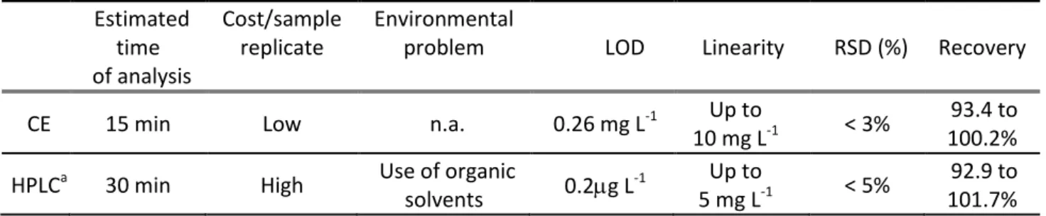
Table I.I. Molecular structure and some physicochemical properties of atrazine…………..….…..1 Table I.II. Molecular structure and some physicochemical properties of EE2………5 Table 1.1. Summary of characteristics for comparison between MEKC and HPLC………..26 Table 2.1. Statistical parameter ( standard errors) for typical analytical curves obtained by UV spectral deconvolution and by MEKC………..38

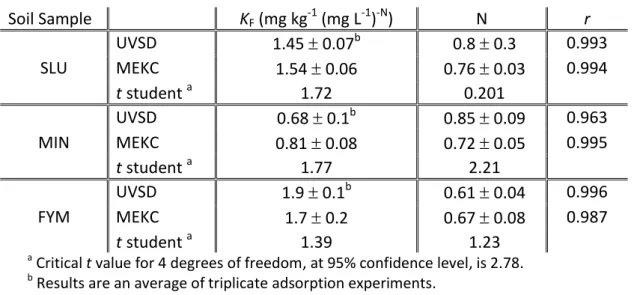
Table 2.2. Mean ( standard errors) Freundlich KF and N parameters for adsorption of

atrazine onto a soil obtained by UVSD and MEKC………..40

Table 2.3. Statistical parameter ( standard errors) for the analytical curves obtained by FSD for each soil sample used………..45

Table 2.4. Recoveries results obtained for EE2 spiked into 0.01 mol L-1 CaCl2 and also into soil

extract solution……….…46

Table 3.1. Schematic list of the synthesized tracers using different methodologies………….….77 Table 3.2. Parameter values obtained for the four-parametric logistic equation (4PL) using

tracer T3: i-Pr/Et/SC3, T5: t-Bu/Cl/C6 and T7: i-Pr/Cl/C6 and polyclonal antibody C193……….86

Table 3.3. Parameter values obtained for the four-parametric logistic equation (4PL) using

different dilutions of polyclonal antibody C193 and tracer T3: i-Pr/Et/SC3………..89

Table 3.4. Atrazine mean concentration and respective RSD for 4 standards (n = 32) ………...92 Table 3.5. Cross-reactivities (CR [%]) of some selected triazine herbicides and their main

metabolites at the center points of their calibration curves……….93

Table 3.6. Mean ( standard errors) Freundlich KF and N parameters for adsorption of

atrazine onto a luvisol soil amended with sewage sludge. Concentration measurements by ELISA and MEKC, respectively………...95

Table 4.1. Influence of long-term application of different organic fertilizers and mineral

fertilizer, respectively, on chemical soil parameters; (MIN – mineral fertilizer; FYM – farmyard manure; SLU – sewage sludge fertilizer; COM – compost fertilizer)………..………….105

(22)

COM – compost fertilizer)……….107

Table 4.3. Calibration parameters for the eleven quantified phenolic compounds. Values are

presented as average ± standard deviation (n=3)……….…112

Table 4.4. Phenolic compound contents of soil samples subjected to the application of

different fertilizers. Values are presented as average ± standard deviation (n=3)………112

Table 5.1. Parameters of the Freundlich equation describing the adsorption isotherms of

atrazine to the four soils samples used………125

Table 5.2. Correlation coefficients (r) between the parameter KF or KFOC and TOC or relative

area distribution (% of total spectrum area) of solid-state 13C CPMAS-NMR spectra………….126

Table 5.3. Parameters of the Freundlich equation describing the desorption isotherms of

atrazine to the four soils samples used (MIN – mineral fertilizer; SLU – sewage sludge fertilizer; FYM – farmyard manure; COM – compost fertilizer)……….…….130

Table 5.4. Parameters obtained for the adsorption isotherm fitting with Hill equation……..136 Table 5.5. Correlation coefficients (r) between Parameter K1 or K1OC and TOC or Relative Area

Distribution (Percent of Total Spectrum Area) of Solid-State 13C CPMAS-NMR Spectra……...140

Table 6.1. Parameter values obtained for the four-parametric logistic equation (4PL) using

atrazine standards prepared with and without HA……….159

Table 6.2. Parameters of linear regression for determination of atrazine recovery rates in

surface and waste water……….164

Table 6.3. Atrazine concentrations (± standard deviation)………165 Table 6.4. Parameter values obtained for the 4PL equation using different dilutions of

polyclonal antibody and tracer for EE2……….167

Table 6.5. Cross-reactivities (CR, %) of some selected hormones at the center points of

their calibration curves………..…….170

Table 6.6. Parameter values obtained for the 4PL equation using EE2 standards prepared

with and without HA………..…….…………....171

(23)

4PL – Four-parameter logistic equation Ab – Antibodies

AHI – Apparent Hysteresis Index BSA – Bovine Serum Albumin CE – Capillary Electrophoresis

COM – Soil fertilized with compost from organic household waste

COM_LOI – soil fertilized with compost from organic household waste and subjected to loss on ignition

CPMAS-NMR – Cross-Polarization Magic-Angle Spinning Nuclear Magnetic Resonance

CR – Cross Reactivity CV – Coefficient of Variation

CZE – Capillary Zone Electrophoresis DAD – Diode Array Detector

DCC – N,N′-Dicyclohexylcarbodiimide DMF – Dimethylformamide

DOC – Dissolved Organic Carbon E1 – Estrone

E2 – 17β-estradiol E3 – Estriol

EDCs – Endocrine Disrupting Compounds EE2 – 17α-ethinylestradiol

ELISA – Enzyme-Linked Immunosorbent Assay EU – European Union

Fab – Fragment containing the antibody binding site Fc – Fragment that crystallizes

FSD – Fluorescence Spectral Deconvolution FT-IR – Fourier Transform Infrared Spectroscopy FYM – Soil fertilized with farmyard manure

(24)

HA – Humic Acids HF – Hydrofluoric acid

HF-LPME – Hollow-Fiber Liquid Phase Microextraction HOC – Hydrophobic Organic Compounds

HOP – Hydrophobic Organic Pollutants

HPLC – High Performance Liquid Chromatography HRP – Horseradish Peroxidase IBCF – Isobutylchloroformiate Ig – Immunoglobulin i-Pr/Cl/C6 – 2-[(1-carboxypent-5-yl)amino]-4-chloro-6-(isopropylamino)-1,3,5-triazine i-Pr/Et/C6 – 2-[(1-carboxypent-5-yl)amino]-4-(ethylamino)-6-(isopropylamino)-1,3,5-triazine i-Pr/Et/SC3 – 2-[(1-carboxyeth-2-yl-)thio]-4-(ethylamino)-6-(isopropylamino)-1,3,5-triazine IS – Internal Standard LC – Liquid Chromatography Lin – Linearity

LOD – Limit Of Detection LOI – Loss On Ignition

LOQ – Limit Of Quantification LSC – Liquid Scintillation Counting

MEKC – Micellar Electrokinetic Chromatography MIN – Soil fertilized with mineral fertilizer MIPs – Molecularly Imprinted Polymers MS – Mass Spectrometer

NHS – N-hydroxysuccinimide

NMR – Nuclear Magnetic Resonance Spectroscopy OC – Organic Carbon

OD – Optical Density

(25)

PPCPs – Phamaceuticals and Personal Care Products ppm – part per million

ppt – part per trillion REF – Reference Spectra RIA – Radioimmunoassay

RSD – Relative Standard Deviation

RSDb – Relative Standard Deviation of the slope

RSWE – Raw soil water extract RT – Room Temperature S/V – Syringic-to-Vanillic unities SDS – Sodium Dodecyl Sulphate

SLU – Soil fertilized with sewage sludge from municipal water treatment facilities SOM – Soil Organic Matter

SPE – Solid Phase Extraction STPs – Sewage Treatment Plants

t-Bu/Cl/C6 – 2-(tert-butylamino)-4-[(1-carboxypent-5-yl)amino]-6-chloro-1,3,5-triazine t-Bu/Et/C6–2-(tert-butylamino)-4-[(1-carboxypent-5-yl)amino]-6-(ethylamino)-1,3,5-triazine t-Bu/Et/SC3 – 2-(tert-butylamino)-4-[(1-carboxyeth-2-yl-)thio]-6-(ethylamino)-1,3,5-triazine THF – Tetrahydrofuran TMB – Tetramethylbenzidine TN – Total Nitrogen

TOC – Total Organic Carbon TOM – Total Organic Matter UV-Vis – Ultraviolet-visible

(26)

a – is the intercept of the regression line

A – OD of a zero control

ai – contribution coefficient of the ith REF in the linear combination

b – empirical parameter which varies with the degree of heterogeneity

B – slope at the inflection point B/B0 – Normalized OD

C – concentration value at the inflection point

Ce – solution-phase concentration (mg L-1)

Cstandard – parameter of the 4PL giving the antigen concentration at the inflection point

Ctest – parameter of the 4PL giving the antigen concentration of the cross-reacting

compound at its inflection point D – OD at a standard excess

K1 – affinity parameter

K1OC – normalized affinity parameter (K1) to total organic content Kd – sorption partition coefficient (L kg-1)

KF – Freundlich distribution coefficient (mg kg-1)(mg L-1)-N

KFdes – Desorption Freundlich distribution coefficient (mg kg-1)(mg L-1)-N

KFOC – Freundlich distribution coefficient normalized to soil organic carbon (mg kg-1)(mg L-1)-N

KFOCdes - Desorption Freundlich distribution coefficient normalized to soil organic carbon (mg

kg-1)(mg L-1)-N

KOC – sorption coefficient normalized to soil organic carbon (L Kg-1)

KOW – octanol-water partition coefficient

Log KOW – logarithmic octanol-water partition coefficient

Mol. Wt. – Molecular weight (g mol-1) N – isotherm nonlinearity factor

Ndes – Desorption isotherm nonlinearity factor OD – optical density

p – number of reference spectra

(27)

REF – Reference Spectra

SS – Sample absorbance Sw – Solubility in water (mg L-1)

(28)

PART I

(29)

(30)

Hydrophobic organic pollutants ... 1 Atrazine ... 1 Description ... 1 Sources of pesticides in waters ... 2 17α-Ethinylestradiol ... 4 Description ... 4 Sources of estrogens in waters ... 5 Fate of HOP in the environment ... 6 References ... 11

(31)

Hydrophobic organic pollutants

Large amounts of chemicals reach the environment via industrial discharges and/or other anthropogenic activities. Hydrophobic organic compounds (HOC), due to their physicochemical properties and their ability to accumulate in the environment, attract the attention of a large number of researchers. Among the so-called hydrophobic organic pollutants (HOP), herbicides, such as atrazine, have been frequently found in soils and surface waters (Yang et al., 2009). Estrogenic compounds, such as 17α-ethinylestradiol, with low water solubility, and thus considered non-polar hydrophobic compounds, have also been detected, becoming problematic for the environment (Feng et al., 2010).

Atrazine

Description

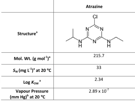
Atrazine (2-chloro-4-ethylamino-6-isopropylamino-s-triazine) is a weak-base selective herbicide with a pKa of 1.7 (Table I.I.) used to control annual grasses and broadleaf weeds in corn and sorghum (Mersie and Seybold, 1996; Smith et al., 2003).

Table I.I. Molecular structure and some physicochemical properties of atrazine Atrazine Structurea Mol. Wt. (g mol-1)a 215.7 SW (mg L-1)a at 20 ºC 33 Log KOW a 2.34 Vapour Pressure (mm Hg)b at 20 ºC 2.89 x 10-7 a Prata et al., 2003 b Kovaios et al., 2006

(32)

Atrazine is relatively hydrophobic presenting a logarithmic octanol-water partition coefficient (log KOW) of 2.34 and a relatively low solubility (33 mg L-1). From properties

presented in Table I.I., it may also be concluded that atrazine is a compound with low volatility.

When applied in agricultural fields it is adsorbed mainly by the shoots and then by the roots and its mechanism of action is based on the inhibition of photosynthesis by binding to specific sites within the plant’s chloroplasts and preventing electron transport process (Kovaios et al., 2006; Nemeth-Konda et al., 2002). Even though this herbicide has been banned in some countries due to its resistance against chemical and biological degradation, and therefore accumulate in the environment (Celano et al., 2008), the application is yet allowed in many countries (more than 80) to control weeds. It is still one of the most widely used herbicides, with a worldwide production of over 70 million kg annually (Ben-Hur et al., 2003; Yang et al., 2009). As a result of its extensive use, atrazine and metabolites have been detected at alarmingly high concentrations in soils, groundwater, rivers and lakes (Celano et al., 2008), being one of the most important pollutants found in groundwater of many countries (Correia et al., 2007). The Directive 98/83/EC has set the maximum concentration of atrazine to 0.1 µg L-1 and the total concentration for all pesticides to 0.5 µg L-1 in what concerns to quality of the water for human consumption (Kovaios et al., 2006). Atrazine was banned in the European Union (EU) in 2004 (Directive 2004/248/CE) because of its persistent groundwater contamination (Ackerman, 2007). In the United States, however, atrazine is one of the most widely used herbicides, where nearly 30 million kg is applied each year (Yang et al., 2009). Several effects of atrazine have been reported, such as increase risk of cancer in humans, induce several hormonal disturbances in amphibians and tumors in rats. However, these are still controversial conclusions (Kovaios et al., 2006; Yang et al., 2009).

Sources of pesticides in waters

Pesticides have been found in water samples, and even in ground waters, at high concentrations (Loos et al., 2010). Many of these substances are introduced into the

(33)

aquatic system through different pathways. The reduction of water contamination by pesticides is only possible if such pathways are known.

Different possibilities are illustrated on Figure I.I. Pesticides can be used either on agriculture or in urban areas. One of the important pathways for pesticide transport is the spray drift during application, surface runoff and leaching during rain events into aquatic systems (Figure I.I., source 1). If farmers are not careful during critical operations, such as filling of sprayers, washing of measuring utilities, disposal of packing material or unused products and cleaning of spraying equipment, they can cause an immediate input of pesticides into the sewerage, septic tank or surface waters (Figure I.I., source 2). Most of pesticides are not significantly eliminated in sewage treatment plants (STPs) and usually end up on effluents’ receiving waters.

Figure I.I. Major pathways for pesticide transport into waters (Gerecke et al., 2002)

Contamination caused by application on urban areas has almost the same causes as the ones described above. Inappropriate operations performed, for example, by gardeners (Figure I.I., source 3), or pesticides present in building materials to prevent

(34)

biological deterioration (Figure I.I., source 4) can be leached during rain events and end up on sewage treatment plants or surface waters. Pesticides applied on lawns, streets, places or roads that are prone to be flushed into sewerage during rain events, are also pathways for pesticide contamination (Figure I.I., source 5). Another source of contamination can occur by products for protection of materials, like bactericide used in soaps that end-up in STPs (Figure I.I., source 6).

17α-Ethinylestradiol

Description

Recently, has been a growing concern about the harmful effects of endocrine disrupting chemicals (EDCs) on the reproduction and development of animals and humans, becoming important the study of their persistence in the environment (Hildebrand et al., 2006). EDCs have been defined as “exogenous agents that interfere with the production, release, transport, metabolism, binding action or elimination of the natural hormones in the body (of a human and/or wildlife species) responsible for the maintenance of homeostasis and the regulation of development process” (Lee et al., 2003). Natural estrogens, such as 17β-estradiol (E2), estrone (E1) and estriol (E3), are predominantly female hormones, biologically active steroid hormones, mainly excreted by humans, but also by livestock (e.g. animal manure) and wildlife (Fan et al., 2007; Feng et al., 2010; Ying et al., 2002; Yu et al., 2004). 17α-ethinylestradiol (EE2), presented in Table I.II., is a manufactured pharmaceutical chemical used for birth control and medical treatments of cancer, hormonal imbalance, osteoporosis, and other ailments (Yu et al., 2004).

Physicochemical properties, such as low water solubility, high log KOW values and low

vapour pressure demonstrate the hydrophobic nature, high sorption potential and low volatility, respectively, of this compound. When present in soils, the behaviour and fate of such compounds is determined by their physicochemical properties. High log KOW values

(35)

4.0 yields medium sorption potential, and log Kow< 2.5 yields low sorption potential

(Jones-Lepp and Stevens, 2007).

Table I.II. Molecular structure and some physicochemical properties of EE2c 17α-ethinylestradiol Structure Mol. Wt. (g mol-1) 296.4 SW (mg L-1) 4.8 Log KOW 4.15 Vapour Pressure (mm Hg) at 20 ºC 4.15 x 10-11 c

Adapted from Ying et al., 2002

Sources of estrogens in waters

Estrogens are compounds of great concern since they can bioaccumulate mainly in the bile and in ovaries of aquatic organisms exposed to contaminated water (Hintemann et al., 2006). These natural and synthetic compounds have gained attention due to their occurrence not only in municipal wastewater, but also in surface and groundwater (Ying et al., 2002).

All humans and animals can excrete hormone steroids from their bodies that will end up in the environment through sewage discharge and animal waste disposal (Ying et al., 2002). Usually they are released in urine as conjugated glucuronides or sulphate complexes (Feng et al., 2010) which are rapidly cleaved and metabolized during transport and treatment of domestic waste, releasing the fully potent hormones with sewage sludge (Emmerik et al., 2003). Women typically excrete 0.5 to 5 g day-1 (up to 400 g

(36)

day-1 for pregnant women), but hormone steroids are also excreted by men. The excretion rate of E1, an important pregnancy estrogen and E2 metabolite, is between 3 and 20 g day-1, while for E3 is up to 64 g day-1 (Racz and Goel, 2010). The daily excretion of EE2 was estimated as being 35 g day-1 (Ying et al., 2002). STPs are not designed to remove estrogens or other micropollutants, thus estrogens that are not degraded during wastewater treatment processes are released into the environment in the effluent (Racz and Goel, 2010). From STPs two products are obtained: one is the liquid effluent and the other is the sludge. The liquid effluent is usually discharged into surface waters or, in some cases, used for irrigation. Sludge, on the other hand, can be disposed in the form of soil amendment or fertilizer. Such disposal can result in leaching of residues present in the sludge into the ground water. Studies have shown that the disposal of animal manures, waste water and sewage sludge to agricultural land can lead to the contamination, by E2 and EE2, of surface and groundwaters (Stumpe and Marschner, 2009). Although the concentrations observed were extremely low (ng L-1) when compared to other anthropogenic organic contaminants, these compounds are extremely potent (Sarmah et al., 2008), particularly EE2 with an estrogenic potency about ten times that of natural hormones. EE2 has been detected in effluents of different STPs (up to 94 ng L-1) (Feng et al., 2010; Stumpe and Marschner, 2009; Yu et al., 2004) and in surface waters (up to 7 ng L-1) (Sarmah et al., 2008).

Fate of HOP in the environment

Aquatic environment is particularly sensitive to pollution, thus drinking water and aquatic organisms also pose a direct threat to human health. The prediction of the aquatic fate of HOP and their distribution in the environment is, therefore, of great importance. Most of these compounds have very low solubility in water (Shim et al., 2007). The water phase is energetically unfavorable for hydrophobic pollutants, thus these tend to associate with organic phases, such as sediments and biological tissues, or to escape from the aqueous phase to the atmosphere.

(37)

Once the organic pollutants reach the soil they can undergo different pathways: volatilize, leach and degrade, among others (Haygarth and Jarvis, 2002), which are represented on Figure I.II.

Figure I.II. Pathways of pollutants degradation and transport.

Pollutants that enter the soil environment are subjected to a diversity of degradative and transport processes. Environmental transport of pollutants comprises distinct processes, such as volatilization, leaching and surface runoff. Pesticides are immediately subjected to volatilization during the application to agricultural soils. Pollutants, when present in soils, can volatilize at higher rates if they are not adsorbed to soil (Haygarth and Jarvis, 2002).

Another fundamental soil process, related to environmental transport of pollutants, is the leaching, where pollutants, dissolved or suspended in soil solution phase, are lost from the soil profile by the action of percolating liquid water. This process has been identified as the major cause of groundwater contamination. Surface runoff has also impact on surface and groundwater quality and has been a major concern for the last three decades (Haygarth and Jarvis, 2002). Pesticide runoff includes dissolved, suspended

(38)

particulate and sediment-adsorbed pesticide that is transported by water from a polluted surface (Haygarth and Jarvis, 2002).

Pollutants degradation is one of the main loss processes of pollutants in the soil. These losses may be due to biological degradation, where microorganisms mediate the transformation process of the pollutant. However, abiotic degradation is often seen as the prevailing process for pollutants degradation and includes hydrolysis, oxidation-reduction and photolysis. Hydrolytic degradation occurs in soil pore water or on surface of clay minerals, while photolysis is due to their exposure to radiation. Although photolysis was not considered, initially, as an important degradation pathway for pollutants in soils, recently, evidence suggests that photoinduced transformations can, in some cases, be significant (Haygarth and Jarvis, 2002).

Retention phenomena comprise several mechanisms, such as sorption-desorption, sequestration and bound residue formation. Sorption and sequestration can be considered as one process, initially fast and then gradually becoming slower. Sorption comprises the physical-chemical processes throughout the pollutant molecule present in soil solution binds to the soil particles. This binding can vary from complete reversibility to total irreversibility and interaction may be physical (van der Waals forces) and/or chemical (electrostatic interactions). One or more of these mechanisms can occur simultaneously. Chemical reactions often lead to the formation of stable chemical linkages, increasing the persistence of the residue in soil. On the other hand, this linkage cause the loss of the chemical identity and, from a toxicological point of view, will lead to: a decrease of its availability to interact with biota; a reduction in the toxicity of the compound; and an immobilization of the compound, thereby reducing its leaching and transport. The extent of sorption depends on several factors, such as properties of soil and pollutant, which include size, shape, configuration, molecular structure, chemical functions, solubility and polarity, among others (Correia et al., 2007; Haygarth and Jarvis, 2002).

Sorption of a pollutant can be divided into fast and slow phase. The fast sorption phase includes surface processes, while slow phase refers to diffusion into and out of humic substances. A very slow diffusion also leads to a very slow release of the pesticide,

(39)

since desorption from the interior of the humic matrix back into solution is more difficult. When desorption is too slow, the pollutant can be considered to be irreversibly adsorbed and named “bound residue” fraction. Bound residues formation plays an important role in the dissipation of hydrophobic pollutants in soil (Prata et al., 2003). Sorption isotherms are mathematical equations widely used to describe retention of chemicals by soils components (Hinz, 2001). A difference between sorption-desorption isotherms is a phenomenon frequently observed and denominated hysteresis. Sorption-desorption hysteresis is usually explained by irreversible chemical binding, sequestration of a solute into specific components of the soil organic matter, or entrapment of the solute into microporous structures or into the soil organic matter (SOM) matrix (Chefetz et al., 2004). Pollutant sorption to soil is often described using a distribution constant of the pollutant between the soil and the solution at the equilibrium, Kd (Spark and Swift, 2002).

The partition coefficient describes an apparent sorption constant that is time, soil, and pesticide dependent (Smith et al., 2003). High values of Kd indicate a strong adsorption of

the pollutant by the soil, and also resistant to microbial degradation (Wauchope et al., 2002). Generally, there is a high correlation between organic matter content of the soils and the distribution constant. Thus, such observation leads to a theory that soil organic matter is the main sorbent in soils, attracting pollutants because they are normally non-polar organic molecules. Therefore, the soil organic carbon sorption coefficient (KOC) of a

pesticide is calculated by dividing a measured Kd, in a specific soil, by the organic carbon

fraction of the same soil. KOC values are universally measures of the relative potential

mobility of pesticides in soils (Wauchope et al., 2002). Nonionic organic compounds isotherms are usually considered to be linear. However, when sorption is evaluated over a large range of concentrations, the partitioning coefficient of most pollutants is not linear. In order to describe more accurately the isotherms of most organic compounds curvilinear equations should be used (Smith et al., 2003). Simple equations, such as Freundlich or Langmuir isotherms are commonly used to describe the sorption data. Every time such equations are not accurate describing the data, more complex expressions are available. Although Freundlich equation is the most commonly used, it is

(40)

crucial to choose an equation that is suitable for the data obtained experimentally (Hinz, 2001).

As mentioned before, even though there are several factors affecting mobility and fate of organic pollutants in the environment, sorption and desorption are considered the most important ones. A fundamental understanding of adsorption-desorption mechanisms is therefore critical for accurate predictions of the environmental load of released HOP and the effective implementation of remedial strategies. In this work, analytical techniques able to follow adsorption-desorption mechanisms of organic pollutants to soil organic matter were developed and optimized. Such techniques were then applied to follow the phenomena in different soil samples (previously characterized) and correlations between content and type of organic matter and its sorption capacity were evaluated.

(41)

References

Ackerman, F., 2007. The economics of atrazine. Int. J. Occup. Environ. Health 13, 441-449.

Ben-Hur, M., Letey, J., Farmer, W.J., Williams, C.F., Nelson, S.D., 2003. Soluble and solid organic matter effects in atrazine adsorption in cultivated soils. Soil Sci. Soc. Am. J. 67, 1140-1146. Celano, G., Šmejkalová, D., Spaccini, R., Piccolo, A., 2008. Interactions of three s-triazines with

humic acids of different structure. J. Agr. Food Chem. 57, 7360-7366.

Chefetz, B., Bilkis, Y.I., Polubesova, T., 2004. Sorption-desorption behaviour of atrazine and phenylurea herbicides in Kishon river sediments. Water Res. 38, 4383-4394.

Correia, F.V., Macrae, A., Guilherme, L.R.G., Langenbach, T., 2007. Atrazine sorption and fate in a Ultisol from humid tropical Brazil. Chemosphere 67, 847-854.

Emmerik, T.V., Angove, M.J., Johnson, B.B., Wells, J.D., Fernandes, M.B., 2003. Sorption of 17β-estradiol onto selected soil minerals. J. Colloid Interf. Sci. 266, 33-39.

Fan, Z., Casey, F.X.M., Hakk, H., Larsen, G., 2007. Persistence and fate of 17β-estradiol and testosterone in agricultural soils. Chemosphere 67, 886-895.

Feng, Y., Zhang, Z., Gao, P., Su, H., Yu, Y., Ren, N., 2010. Adsorption behaviour of EE2 (17α-ethinylestradiol) onto the inactivated sewage sludge: Kinetics, thermodynamics and influence factors. J. Hazard. Mater. 175, 970-976.

Gerecke, A.C., Schärer, M., Singer, H.P., Mϋller, S.R., Schwarzenbach, R.P., Sägesser, M., Ochsenbein, U., Popow, G., 2002. Sources of pesticides in surface waters in Switzerland: pesticide load through waste water treatment plants – current situation and reduction potential. Chemosphere 48, 307-315.

Haygarth, P.M., Jarvis, S.C., 2002. Agriculture, hydrology and water quality. CABI Publishing, First Edition, Wallingford, UK.

Hildebrand, C., Londry, K.L., Farenhorst, A., 2006. Sorption and desorption of three endocrine disrupters in soils. J. Environ. Sci. Heal. B 41, 907-921.

Hintemann, T., Schneider, C., Schöler, H.F., Schneider, R.J., 2006. Field study using two immunoassays for the determination of estradiol and ethinylestradiol in the aquatic environment. Water Res. 40, 2287-2294.

Hinz, C., 2001. Description of sorption data with isotherm equations. Geoderma 99, 225-243. Jones-Lepp, T.L., Stevens, R., 2007. Pharmaceuticals and personal care products in

biosolids/sewage sludge: interface between analytical chemistry and regulation. Anal.

(42)

Kovaios, I.D., Parakeva, C.A., Koutsoukos, P.G., Payatakes, A.C., 2006. Adsorption of atrazine on soils: Model study. J. Colloid Interf. Sci. 299, 88-94.

Lee, L.S., Strock, T.J., Sarmah, A.K., Rao, P.S.C., 2003. Sorption and dissipation of testosterone, estrogens, and their primary transformation products in soils and sediment. Environ. Sci.

Technol. 37, 4098-4105.

Loos, R., Locoro, G., Comero, S., Contini, S., Schwesig, D., Werres, F., Balsaa, P., Gans, O., Weiss, S., Blaha, L., Bolchi, M., Gawlik, B.M., 2010. Pan-European survey on the occurrence of selected polar organic persistent pollutants in ground water. Water Res. 44, 4115-4126.

Mersie, W., Seybold, C., 1996. Adsorption and desorption of atrazine, deethylatrazine, deisopropylatrazine, and hydroxyatrazine on levy wetland soil. J. Agr. Food Chem. 44, 1925-1929.

Nemeth-Konda, L., Füleky, G., Morovjan, G., Csokan, P., 2002. Sorption behaviour of acetochlor, atrazine, carbendazim, diazinon, imidacloprid and isoproturon on Hungarian agricultural soil.

Chemosphere 48, 545-552.

Prata, F., Lavorenti, A., Vanderborght, J., Burauel, P., Vereecken, H., 2003. Miscible displacement, sorption and desorption of atrazine in a Brazilian oxisol. Vadose Zone J. 2, 728-738.

Racz, L., Goel, R.K., 2010. Fate and removal of estrogens in municipal wastewater. J. Environ.

Monit. 12, 58-70.

Sarmah, A.K., Northcott, G.L., Scherr, F.F., 2008. Retention of estrogenic steroid hormones by selected New Zealand soils. Environ. Int. 34, 749-755.

Shim, J.-K., Park, I.-S., Kim, J.-Y., 2007. Use of amphiphilic polymer nanoparticles as a nano-absorbent for enhancing efficiency of micelle-enhanced ultrafiltration process. J. Ind. Eng.

Chem. 13, 917-925.

Smith, M.C., Shaw, D.R., Massey, J.H., Boyette, M., Kingery, W., 2003. Using nonequilibrium thin-disc and batch equilibrium techniques to evaluate herbicide sorption. J. Environ. Qual. 32, 1393-1404.

Spark, K.M., Swift, R.S., 2002. Effect of soil composition and dissolved organic matter on pesticide sorption. Sci. Total Environ. 298, 147-161

Stumpe, B., Marschner, B., 2009. Factors controlling the biodegradation of 17α-estradiol, estrone and 17α-ethinylestradiol in different natural soils. Chemosphere 74, 556-562.

Wauchope, R.D., Yeh, S., Linders, J.B.H.J., Kloskowski, R., Tanaka, K., Rubin, B., Katayama, A., Kordel, W., Gerstl, Z., Lane, M., Unsworth, J.B., 2002. Pesticide soil sorption parameters: theory, measurement, uses, limitations and reliability. Pest. Manag. Sci. 58, 419-445.

(43)

Yang, W., Zhang, J., Zhang, C., Zhu, L., Chen, W., 2009. Sorption and resistant desorption of atrazine in typical Chinese soils. J. Environ. Qual. 38, 171-179.

Ying, G.-G., Kookana, R.S., Ru, Y.-J., 2002. Occurance and fate of hormone steroids in the environment. Environ. Int. 28, 545-551.

Yu, Z., Xiao, B., Huang, W., Peng, P., 2004. Sorption of steroid estrogens to soils and sediments.

(44)

PART II

DEVELOPMENT OF ANALYTICAL PROCEDURES TO

FOLLOW SORPTION BEHAVIOUR OF HOP ONTO SOILS

(45)

CHAPTER 1

(46)

ATRAZINE ANALYSIS BY CAPILLARY ELECTROPHORESIS*

1.1. Introduction ... 15 1.2. Experimental procedure ... 16 1.2.1. Soil sample ... 16 1.2.2. Instrumentation ... 17 1.2.3. Buffer and standards ... 18 1.2.4. Capillary column conditioning ... 18 1.2.5. Separation conditions ... 19 1.2.6. Suitability of the MEKC method ... 19 1.2.7. Adsorption studies ... 19 1.2.8. Data analysis ... 20 1.3. Results and discussion ... 21 1.3.1. Electrophoretic separation of atrazine ... 21 1.3.2. Performance of the method ... 22 1.3.3. Preliminary studies and kinetics experiments ... 23 1.3.4. Adsorption studies ... 24 1.3.5. MEKC and HPLC methods – comparison ... 26 1.4. Conclusions ... 28 1.5. References ... 29