An expansion formula with higher-order derivatives for fractional operators of variable order

(1)

Volume 2013, Article ID 915437,11pages http://dx.doi.org/10.1155/2013/915437

Research Article

An Expansion Formula with Higher-Order Derivatives for

Fractional Operators of Variable Order

Ricardo Almeida and Delfim F. M. Torres

Center for Research and Development in Mathematics and Applications (CIDMA), Department of Mathematics, University of Aveiro, 3810-193 Aveiro, Portugal

Correspondence should be addressed to Delfim F. M. Torres; [email protected] Received 27 August 2013; Accepted 19 September 2013

Academic Editors: A. Atangana, S. C. O. Noutchie, and A. Secer

Copyright © 2013 R. Almeida and D. F. M. Torres. This is an open access article distributed under the Creative Commons Attribution License, which permits unrestricted use, distribution, and reproduction in any medium, provided the original work is properly cited.

We obtain approximation formulas for fractional integrals and derivatives of Riemann-Liouville and Marchaud types with a variable fractional order. The approximations involve integer-order derivatives only. An estimation for the error is given. The efficiency of the approximation method is illustrated with examples. As applications, we show how the obtained results are useful to solve differential equations, and problems of the calculus of variations that depend on fractional derivatives of Marchaud type.

1. Introduction

Fractional calculus is a natural extension of the integer-order calculus by considering derivatives and integrals of arbitrary real or complex order 𝛼 ∈ K, with K = R or K = C. The subject was born from a famous cor-respondence between L’Hopital and Leibniz in 1695 and then developed by many famous mathematicians, like Euler, Laplace, Abel, Liouville, and Riemann, just to mention a few names. Recently, fractional calculus has attracted the attention of a vast number of researchers, not only in mathematics, but also in physics and in engineering, and has proven to better describe certain complex phenomena in nature [1,2].

Since the order𝛼 of the integrals and derivatives may take any value, another interesting extension is to consider the order not as a constant during the process but as a variable 𝛼(𝑡) that depends on time. This provides an extension of the classical fractional calculus and it was introduced by Samko and Ross in 1993 [3] (see also [4]). The variable order fractional calculus is nowadays recognized as a useful tool, with successful applications in mechanics, in the modeling of linear and nonlinear viscoelasticity oscillators, and in other phenomena where the order of the derivative varies with time. For more on the subject, and its applications, we

mention [5–11]. For a numerical approach see, for example, [12–14]. Results on differential equations and the calculus of variations with fractional operators of variable order can be found in [15, 16] and references therein. In this paper we show how fractional derivatives and integrals of variable order can be approximated by classical integer-order operators.

The outline of the paper is the following. In Section 2 we present the necessary definitions, namely, the fractional operators of Riemann-Liouville and Marchaud of variable order. Some properties of the operators are also given. The main core of the paper is Section 3, where we prove the expansion formulas for the considered fractional operators, with the size of the expansion being the derivative of order 𝑛 ∈ N. InSection 4we show the accuracy of our method with some examples and how the approximations can be applied in different situations to solve problems involving variable order fractional operators.

2. Fractional Calculus of Variable Order

In the following, the order of the fractional operators is given by a function𝛼 ∈ 𝐶1([𝑎, 𝑏], ]0, 1[); 𝑥(⋅) is assumed to ensure convergence for each of the involved integrals. For a complete and rigorous study of fractional calculus we refer to [17].

(2)

Definition 1. Let𝑥(⋅) be a function with domain [𝑎, 𝑏]. Then,

for𝑡 ∈ [𝑎, 𝑏],

(i) the left Riemann-Liouville fractional integral of order 𝛼(⋅) is given by

𝑎𝐼𝑡𝛼(𝑡)𝑥 (𝑡) = _{Γ (𝛼 (𝑡))}1 ∫ 𝑡 𝑎(𝑡 − 𝜏)

𝛼(𝑡)−1_{𝑥 (𝜏) 𝑑𝜏,} ₍₁₎

(ii) the right Riemann-Liouville fractional integral of order𝛼(⋅) is given by

𝑡𝐼𝑏𝛼(𝑡)𝑥 (𝑡) = _{Γ (𝛼 (𝑡))}1 ∫ 𝑏 𝑡 (𝜏 − 𝑡)

𝛼(𝑡)−1_{𝑥 (𝜏) 𝑑𝜏,} ₍₂₎

(iii) the left Riemann-Liouville fractional derivative of order𝛼(⋅) is given by

𝑎𝐷𝛼(𝑡)𝑡 𝑥 (𝑡) = _{Γ (1 − 𝛼 (𝑡))}1 _𝑑𝑡𝑑 ∫ 𝑡 𝑎(𝑡 − 𝜏)

−𝛼(𝑡)_{𝑥 (𝜏) 𝑑𝜏, (3)}

(iv) the right Riemann-Liouville fractional derivative of order𝛼(⋅) is given by

𝑡𝐷𝑏𝛼(𝑡)𝑥 (𝑡) = _{Γ (1 − 𝛼 (𝑡))}−1 _𝑑𝑡𝑑 ∫ 𝑏 𝑡 (𝜏 − 𝑡)

−𝛼(𝑡)_{𝑥 (𝜏) 𝑑𝜏, (4)}

(v) the left Marchaud fractional derivative of order𝛼(⋅) is given by 𝑎D𝛼(𝑡)𝑡 𝑥 (𝑡) = _{Γ (1 − 𝛼 (𝑡)) (𝑡 − 𝑎)}𝑥 (𝑡) 𝛼(𝑡) + 𝛼 (𝑡) Γ (1 − 𝛼 (𝑡))∫ 𝑡 𝑎 𝑥 (𝑡) − 𝑥 (𝜏) (𝑡 − 𝜏)1+𝛼(𝑡)𝑑𝜏, (5)

(vi) the right Marchaud fractional derivative of order𝛼(⋅) is given by 𝑡D𝛼(𝑡)𝑏 𝑥 (𝑡) = _{Γ (1 − 𝛼 (𝑡)) (𝑏 − 𝑡)}𝑥 (𝑡) 𝛼(𝑡) + 𝛼 (𝑡) Γ (1 − 𝛼 (𝑡))∫ 𝑏 𝑡 𝑥 (𝑡) − 𝑥 (𝜏) (𝜏 − 𝑡)1+𝛼(𝑡)𝑑𝜏. (6)

Remark 2. It follows fromDefinition 1that

𝑎𝐷𝛼(𝑡)𝑡 𝑥 (𝑡) = _𝑑𝑡𝑑𝑎𝐼𝑡1−𝛼(𝑡)𝑥 (𝑡) , 𝑡𝐷𝛼(𝑡)𝑏 𝑥 (𝑡) = −_𝑑𝑡𝑑𝑡𝐼𝑏1−𝛼(𝑡)𝑥 (𝑡) .

(7)

Example 3 (see [3]). Let 𝑥 be the power function 𝑥(𝑡) = (𝑡 − 𝑎)𝛾_{. Then, for}_{𝛾 > −1, we have}

𝑎𝐼𝑡𝛼(𝑡)𝑥 (𝑡) = Γ (𝛾 + 1) Γ (𝛾 + 𝛼 (𝑡) + 1)(𝑡 − 𝑎)𝛾+𝛼(𝑡), 𝑎D𝛼(𝑡)𝑡 𝑥 (𝑡) = Γ (𝛾 + 1) Γ (𝛾 − 𝛼 (𝑡) + 1)(𝑡 − 𝑎)𝛾−𝛼(𝑡), 𝑎𝐷𝛼(𝑡)𝑡 𝑥 (𝑡) = _{Γ (𝛾 − 𝛼 (𝑡) + 1)}Γ (𝛾 + 1) (𝑡 − 𝑎)𝛾−𝛼(𝑡) − 𝛼(1)(𝑡) Γ (𝛾 + 1) Γ (𝛾 − 𝛼 (𝑡) + 2)(𝑡 − 𝑎)𝛾−𝛼(𝑡)+1 × [ln (𝑡 − 𝑎) − 𝜓 (𝛾 − 𝛼 (𝑡) + 2) +𝜓 (1 − 𝛼 (𝑡))] , (8)

where 𝜓 is the Psi function, that is, the derivative of the logarithm of the Gamma function:

𝜓 (𝑡) =_𝑑𝑡𝑑 ln(Γ (𝑡)) =Γ

󸀠_(𝑡)

Γ (𝑡). (9)

FromExample 3we see that _𝑎𝐷𝛼(𝑡)_𝑡 𝑥(𝑡) ̸=_𝑎D𝛼(𝑡)_𝑡 𝑥(𝑡). Also, the symmetry on power functions is violated, when we con-sider _𝑎𝐼𝛼(𝑡)_𝑡 𝑥(𝑡) and _𝑎𝐷𝛼(𝑡)_𝑡 𝑥(𝑡), but holds for _𝑎𝐼_𝑡𝛼(𝑡)𝑥(𝑡) and

𝑎D𝛼(𝑡)𝑡 𝑥(𝑡). Later we explain this better, when we deduce the

expansion formula for the Marchaud fractional derivative. In contrast with the constant fractional order case, the law of exponents fails for fractional integrals of variable order. However, a weak form holds (see [3]): if𝛽(𝑡) ≡ 𝛽, 𝑡 ∈]0, 1[, then _𝑎𝐼_𝑡𝛼(𝑡)_𝑎𝐼_𝑡𝛽𝑥(𝑡) = _𝑎𝐼_𝑡𝛼(𝑡)+𝛽𝑥(𝑡).

3. Expansion Formulas with

Higher-Order Derivatives

The main results of the paper provide approximations of the fractional derivatives of a given function𝑥 by sums involving only integer derivatives of 𝑥. The approximations use the generalization of the binomial coefficient formula to real numbers:

(−𝛼 (𝑡)_{𝑘 ) (−1)}𝑘 _{= (𝛼 (𝑡) + 𝑘 − 1}

𝑘 ) = Γ (𝛼 (𝑡) + 𝑘)_{Γ (𝛼 (𝑡)) 𝑘!} . (10) Theorem 4. Fix 𝑛 ∈ N and 𝑁 ≥ 𝑛 + 1, and let 𝑥(⋅) ∈ 𝐶𝑛+1_{([𝑎, 𝑏], R). Define the (left) moment of 𝑥 of order 𝑘 by}

𝑉_𝑘(𝑡) = (𝑘 − 𝑛) ∫𝑡

𝑎(𝜏 − 𝑎)

𝑘−𝑛−1_{𝑥 (𝜏) 𝑑𝜏.} ₍₁₁₎

Then,

(3)

with 𝑆1(𝑡) = (𝑡 − 𝑎)−𝛼(𝑡)[ 𝑛 ∑ 𝑘=0𝐴 (𝛼 (𝑡) , 𝑘) (𝑡 − 𝑎) 𝑘_𝑥(𝑘)_(𝑡) + ∑𝑁 𝑘=𝑛+1𝐵 (𝛼 (𝑡) , 𝑘) (𝑡 − 𝑎) 𝑛−𝑘_𝑉 𝑘(𝑡)] , (13) where 𝐴 (𝛼 (𝑡) , 𝑘) =_{Γ (𝑘 + 1 − 𝛼 (𝑡))}1 × [ [ 1 + ∑𝑁 𝑝=𝑛+1−𝑘 Γ (𝑝 − 𝑛 + 𝛼 (𝑡)) Γ (𝛼 (𝑡) − 𝑘) (𝑝 − 𝑛 + 𝑘)!]_], 𝑘 = 0, . . . , 𝑛, 𝐵 (𝛼 (t) , 𝑘) = _{Γ (−𝛼 (𝑡)) Γ (1 + 𝛼 (𝑡)) (𝑘 − 𝑛)!}Γ (𝑘 − 𝑛 + 𝛼 (𝑡)) , 𝑆₂(𝑡) = 𝑥 (𝑡) 𝛼(1)(𝑡) Γ (1 − 𝛼 (𝑡))(𝑡 − 𝑎)1−𝛼(𝑡) × [ln(𝑡 − 𝑎) 1 − 𝛼 (𝑡) − 1 (1 − 𝛼 (𝑡))2 − ln (𝑡 − 𝑎)∑𝑁 𝑘=0 (−𝛼 (𝑡)_{𝑘 )}(−1)𝑘 𝑘 + 1 +∑𝑁 𝑘=0 (−𝛼 (𝑡)_{𝑘 ) (−1)}𝑘∑𝑁 𝑝=1 1 𝑝 (𝑘 + 𝑝 + 1)] + 𝛼(1)(𝑡) Γ (1 − 𝛼 (𝑡))(𝑡 − 𝑎)1−𝛼(𝑡) × [ln (𝑡 − 𝑎)𝑁+𝑛+1∑ 𝑘=𝑛+1 ( −𝛼 (𝑡)_{𝑘 − 𝑛 − 1)} × (−1)_{𝑘 − 𝑛}𝑘−𝑛−1(𝑡 − 𝑎)𝑛−𝑘𝑉_𝑘(𝑡) −𝑁+𝑛+1∑ 𝑘=𝑛+1 ( −𝛼 (𝑡)_{𝑘 − 𝑛 − 1) (−1)}𝑘−𝑛−1 × ∑𝑁 𝑝=1 1 𝑝 (𝑘 + 𝑝 − 𝑛)(𝑡 − 𝑎)𝑛−𝑘−𝑝𝑉𝑘+𝑝(𝑡)] . (14)

The error of the approximation _𝑎𝐷𝛼(𝑡)_𝑡 𝑥(𝑡) ≈ 𝑆₁(𝑡) − 𝑆₂(𝑡) is given by𝐸_1,𝑁(𝑡) + 𝐸_2,𝑁(𝑡), where 𝐸_1,𝑁(𝑡) and 𝐸_2,𝑁(𝑡) are bounded by 󵄨󵄨󵄨󵄨𝐸1,𝑁(𝑡)󵄨󵄨󵄨󵄨 ≤ 𝐿𝑛+1(𝑡) × exp((𝑛 − 𝛼 (𝑡)) 2_{+ 𝑛 − 𝛼 (𝑡))} Γ (𝑛 + 1 − 𝛼 (𝑡)) (𝑛 − 𝛼 (𝑡)) 𝑁𝑛−𝛼(𝑡) × (𝑡 − 𝑎)𝑛+1−𝛼(𝑡)_, ₍₁₅₎ 󵄨󵄨󵄨󵄨𝐸2,𝑁(𝑡)󵄨󵄨󵄨󵄨 ≤ 𝐿1(𝑡)󵄨󵄨󵄨󵄨_󵄨𝛼(1)(𝑡)󵄨󵄨󵄨󵄨_{󵄨 (𝑡 − 𝑎)}2−𝛼(𝑡)exp(𝛼2(𝑡) − 𝛼 (𝑡)) Γ (2 − 𝛼 (𝑡)) 𝑁1−𝛼(𝑡) × [|ln (𝑡 − 𝑎)| +_𝑁1] (16) with 𝐿_𝑗(𝑡) = max 𝜏∈[𝑎,𝑡]󵄨󵄨󵄨󵄨󵄨𝑥 (𝑗)_(𝜏)󵄨󵄨󵄨󵄨 󵄨 , 𝑗 ∈ {1, 𝑛 + 1} . (17)

Proof. Starting with equality

𝑎𝐷𝛼(𝑡)𝑡 𝑥 (𝑡) = _{Γ (1 − 𝛼 (𝑡))}1 _𝑑𝑡𝑑 ∫ 𝑡 𝑎(𝑡 − 𝜏)

−𝛼(𝑡)_{𝑥 (𝜏) 𝑑𝜏, (18)}

doing the change of variable𝑡 − 𝜏 = 𝑢 − 𝑎 over the integral, and then differentiating it, we get

𝑎𝐷𝛼(𝑡)𝑡 𝑥 (𝑡) = _{Γ (1 − 𝛼 (𝑡))}1 _𝑑𝑡𝑑 ∫ 𝑡 𝑎(𝑢 − 𝑎) −𝛼(𝑡)_{𝑥 (𝑡 − 𝑢 + 𝑎) 𝑑𝑢} = 1 Γ (1 − 𝛼 (𝑡))[(𝑡 − 𝑎)𝑥 (𝑎)𝛼(𝑡) + ∫𝑡 𝑎 𝑑 𝑑𝑡[(𝑢 − 𝑎)−𝛼(𝑡) ×𝑥 (𝑡 − 𝑢 + 𝑎)] 𝑑𝑢] = 1 Γ (1 − 𝛼 (𝑡)) × [ 𝑥 (𝑎) (𝑡 − 𝑎)𝛼(𝑡) + ∫ 𝑡 𝑎[−𝛼 (1)_{(𝑡) (𝑢 − 𝑎)}−𝛼(𝑡) × ln (𝑢 − 𝑎) 𝑥 (𝑡 − 𝑢 + 𝑎) + (𝑢 − 𝑎)−𝛼(𝑡) × 𝑥(1)(𝑡 − 𝑢 + 𝑎)] 𝑑𝑢] = 𝑆₁(𝑡) − 𝑆₂(𝑡) (19) with 𝑆₁(𝑡) = 1 Γ (1 − 𝛼 (𝑡))[(𝑡 − 𝑎)𝑥 (𝑎)𝛼(𝑡) + ∫ 𝑡 𝑎(𝑡 − 𝜏) −𝛼(𝑡)_𝑥(1)_{(𝜏) 𝑑𝜏] ,} (20) 𝑆₂(𝑡) = 𝛼(1)(𝑡) Γ (1 − 𝛼 (𝑡))∫ 𝑡 𝑎(𝑡 − 𝜏) −𝛼(𝑡)_ln_{(𝑡 − 𝜏) 𝑥 (𝜏) 𝑑𝜏.} (21)

(4)

The equivalence between (20) and (13) follows from the computations of [18]. To show the equivalence between (21) and (14) we start in the same way as done in [19], to get

𝑆₂(𝑡) = 𝛼(1)(𝑡) Γ (1 − 𝛼 (𝑡))[𝑥 (𝑡) ∫ 𝑡 𝑎(𝑡 − 𝑢) −𝛼(𝑡)_ln_{(𝑡 − 𝑢) 𝑑𝑢} − ∫𝑡 𝑎𝑥 (1)_(𝜏) × (∫𝜏 𝑎 (𝑡 − 𝑢) −𝛼(𝑡)_ln_{(𝑡 − 𝑢) 𝑑𝑢) 𝑑𝜏]} = 𝛼(1)(𝑡) Γ (1 − 𝛼 (𝑡))[𝑥 (𝑡) (𝑡 − 𝑎)1−𝛼(𝑡) × [ln(𝑡 − 𝑎) 1 − 𝛼 (𝑡) − 1 (1 − 𝛼 (𝑡))2] − ∫𝑡 𝑎𝑥 (1)_(𝜏) × (∫𝜏 𝑎 (𝑡 − 𝑎) −𝛼(𝑡)_{(1 −}𝑢 − 𝑎 𝑡 − 𝑎) −𝛼(𝑡) × [ ln (𝑡 − 𝑎) + ln (1 −𝑢 − 𝑎 𝑡 − 𝑎)] 𝑑𝑢) 𝑑𝜏] . (22) Now, applying Taylor’s expansion over

(1 −𝑢 − 𝑎_{𝑡 − 𝑎})−𝛼(𝑡) (23) and ln(1 −𝑢 − 𝑎 𝑡 − 𝑎) , (24) we deduce that 𝑆₂(𝑡) = 𝛼(1)(𝑡) Γ (1 − 𝛼 (𝑡)) × [𝑥 (𝑡) (𝑡 − 𝑎)1−𝛼(𝑡)[ln(𝑡 − 𝑎) 1 − 𝛼 (𝑡) − 1 (1 − 𝛼 (𝑡))2] − ∫𝑡 𝑎𝑥 (1)_{(𝜏) ( ∫}𝜏 𝑎 (𝑡 − 𝑎) −𝛼(𝑡)_ln_{(𝑡 − 𝑎)} ×∑𝑁 𝑘=0 (−𝛼 (𝑡)_{𝑘 ) (−1)}𝑘(𝑢 − 𝑎)𝑘 (𝑡 − 𝑎)𝑘𝑑𝑢 − ∫𝜏 𝑎 (𝑡 − 𝑎) −𝛼(𝑡)_∑𝑁 𝑘=0 (−𝛼 (𝑡)_{𝑘 ) (−1)}𝑘 × (𝑢 − 𝑎)𝑘 (𝑡 − 𝑎)𝑘 𝑁 ∑ 𝑝=1 1 𝑝 (𝑢 − 𝑎)𝑝 (𝑡 − 𝑎)𝑝𝑑𝑢) 𝑑𝜏] + 𝐸2,𝑁(𝑡) = 𝛼(1)(𝑡) Γ (1 − 𝛼 (𝑡))[𝑥 (𝑡) (𝑡 − 𝑎)1−𝛼(𝑡) × [ln(𝑡 − 𝑎) 1 − 𝛼 (𝑡) − 1 (1 − 𝛼 (𝑡))2] − ∫𝑡 𝑎𝑥 (1)_{(𝜏) (𝑡 − 𝑎)}−𝛼(𝑡)_ln_{(𝑡 − 𝑎)} ×∑𝑁 𝑘=0 (−𝛼 (𝑡)_{𝑘 )} (−1)𝑘 (𝑡 − 𝑎)𝑘 × (∫𝜏 𝑎 (𝑢 − 𝑎) 𝑘 _{𝑑𝑢) 𝑑𝜏} + ∫𝑡 𝑎𝑥 (1)_{(𝜏) (𝑡 − 𝑎)}−𝛼(𝑡) ×∑𝑁 𝑘=0 (−𝛼 (𝑡)_{𝑘 )} (−1)𝑘 (𝑡 − 𝑎)𝑘 ×∑𝑁 𝑝=1 1 𝑝(𝑡 − 𝑎)𝑝 × (∫𝜏 𝑎 (𝑢 − 𝑎) 𝑘+𝑝 _{𝑑𝑢) 𝑑𝜏]} + 𝐸_2,𝑁(𝑡) = 𝛼(1)(𝑡) (𝑡 − 𝑎)−𝛼(𝑡) Γ (1 − 𝛼 (𝑡)) × [𝑥 (𝑡) (𝑡 − 𝑎) [ln(𝑡 − 𝑎) 1 − 𝛼 (𝑡) − 1 (1 − 𝛼 (𝑡))2] − ln (𝑡 − 𝑎)∑𝑁 𝑘=0 (−𝛼 (𝑡)_{𝑘 )} (−1)𝑘 (𝑡 − 𝑎)𝑘(𝑘 + 1) × (∫𝑡 𝑎𝑥 (1)_{(𝜏) (𝜏 − 𝑎)}𝑘+1 _𝑑𝜏) +∑𝑁 𝑘=0 (−𝛼 (𝑡)_{𝑘 )} (−1)𝑘 (𝑡 − 𝑎)𝑘 𝑁 ∑ 𝑝=1 1 𝑝(𝑡 − 𝑎)𝑝_{(𝑘 + 𝑝 + 1)} × (∫𝑡 𝑎𝑥 (1)_{(𝜏) (𝜏 − 𝑎)}𝑘+𝑝+1_{𝑑𝜏)] + 𝐸} 2,𝑁(𝑡) . (25)

Integrating by parts, we conclude with the two following equalities: ∫𝑡 𝑎𝑥 (1)_{(𝜏) (𝜏 − 𝑎)}𝑘+1_{𝑑𝜏 = 𝑥 (𝑡) (𝑡 − 𝑎)}𝑘+1_{− 𝑉} 𝑘+𝑛+1(𝑡) , ∫𝑡 𝑎𝑥 (1)_{(𝜏) (𝜏 − 𝑎)}𝑘+𝑝+1_{𝑑𝜏 = 𝑥 (𝑡) (𝑡 − 𝑎)}𝑘+𝑝+1_{− 𝑉} 𝑘+𝑝+𝑛+1(𝑡) . (26)

(5)

The deduction of relation (14) for 𝑆₂(𝑡) follows now from direct calculations. Finally, we prove the upper bound for-mula for the error. The bound (15) for the error𝐸_1,𝑁(𝑡) at time 𝑡 follows easily from [18]. With respect to sum𝑆₂, the error at 𝑡 is bounded by 󵄨󵄨󵄨󵄨𝐸2,𝑁(𝑡)󵄨󵄨󵄨󵄨 ≤󵄨󵄨󵄨󵄨󵄨󵄨󵄨󵄨 󵄨 𝛼(1)_{(𝑡) (𝑡 − 𝑎)}−𝛼(𝑡) Γ (1 − 𝛼 (𝑡)) 󵄨󵄨󵄨󵄨󵄨󵄨󵄨󵄨_󵄨 ×󵄨󵄨󵄨󵄨󵄨󵄨󵄨󵄨 󵄨󵄨− ln (𝑡 − 𝑎) ∞ ∑ 𝑘=𝑁+1 (−𝛼 (𝑡)_{𝑘 )}(−1)_{𝑘 + 1}𝑘 × (∫𝑡 𝑎𝑥 (1)_(𝜏)(𝜏 − 𝑎)𝑘+1 (𝑡 − 𝑎)𝑘 𝑑𝜏) + ∑∞ 𝑘=𝑁+1 (−𝛼 (𝑡)_{𝑘 ) (−1)}𝑘 × ∑∞ 𝑝=𝑁+1 1 𝑝 (𝑘 + 𝑝 + 1) × (∫𝑡 𝑎𝑥 (1)_(𝜏)(𝜏 − 𝑎)𝑘+𝑝+1 (𝑡 − 𝑎)𝑘+𝑝 𝑑𝜏) 󵄨󵄨󵄨󵄨 󵄨󵄨󵄨󵄨 󵄨󵄨. (27)

Define the quantities 𝐼₁(𝑡) = ∫∞ 𝑁 1 𝑘1−𝛼(𝑡)_{(𝑘 + 1) (𝑘 + 2)} 𝑑𝑘, 𝐼₂(𝑡) = ∫∞ 𝑁 ∫ ∞ 𝑁 1 𝑘1−𝛼(𝑡)_{𝑝 (𝑘 + 𝑝 + 1) (𝑘 + 𝑝 + 2)} 𝑑𝑝 𝑑𝑘. (28) Inequality (16) follows from relation

󵄨󵄨󵄨󵄨

󵄨󵄨󵄨󵄨(−𝛼 (𝑡)𝑘 )󵄨󵄨󵄨󵄨󵄨󵄨󵄨󵄨 ≤

exp(𝛼2(𝑡) − 𝛼 (𝑡))

𝑘1−𝛼(𝑡) (29)

and the upper bounds 𝐼₁(𝑡) < ∫∞ 𝑁 1 𝑘2−𝛼(𝑡)𝑑𝑘 = 1 (1 − 𝛼 (𝑡)) 𝑁1−𝛼(𝑡), 𝐼₂(𝑡) < ∫∞ 𝑁 ∫ ∞ 𝑁 1 𝑘2−𝛼(𝑡)_𝑝2 𝑑𝑝 𝑑𝑘 = 1 (1 − 𝛼 (𝑡)) 𝑁2−𝛼(𝑡) (30) for𝐼₁and𝐼₂.

Similarly as done in Theorem 4 for the left Riemann-Liouville fractional derivative, an approximation formula can be deduced for the right Riemann-Liouville fractional derivative.

Theorem 5. Fix 𝑛 ∈ N and 𝑁 ≥ 𝑛 + 1, and let 𝑥(⋅) ∈ 𝐶𝑛+1([𝑎, 𝑏], R). Define the (right) moment of 𝑥 of order 𝑘 by

𝑊_𝑘(𝑡) = (𝑘 − 𝑛) ∫𝑏 𝑡 (𝑏 − 𝜏) 𝑘−𝑛−1_{𝑥 (𝜏) 𝑑𝜏.} ₍₃₁₎ Then, 𝑡𝐷𝛼(𝑡)𝑏 𝑥 (𝑡) = 𝑆1(𝑡) + 𝑆2(𝑡) + 𝐸1,𝑁(𝑡) + 𝐸2,𝑁(𝑡) (32) with 𝑆₁(𝑡) = (𝑏 − 𝑡)−𝛼(𝑡)[∑𝑛 𝑘=0𝐴 (𝛼 (𝑡) , 𝑘) (𝑏 − 𝑡) 𝑘_𝑥(𝑘)_(𝑡) + ∑𝑁 𝑘=𝑛+1𝐵 (𝛼 (𝑡) , 𝑘) (𝑏 − 𝑡) 𝑛−𝑘_𝑊 𝑘(𝑡)] , (33) where 𝐴 (𝛼 (𝑡) , 𝑘) = _{Γ (𝑘 + 1 − 𝛼 (𝑡))}(−1)𝑘 × [ [ 1 + ∑𝑁 𝑝=𝑛+1−𝑘 Γ (𝑝 − 𝑛 + 𝛼 (𝑡)) Γ (𝛼 (𝑡) − 𝑘) (𝑝 − 𝑛 + 𝑘)!]_], 𝑘 = 0, . . . , 𝑛, 𝐵 (𝛼 (𝑡) , 𝑘) = _{Γ (−𝛼 (𝑡)) Γ (1 + 𝛼 (𝑡)) (𝑘 − 𝑛)!}(−1)𝑛+1Γ (𝑘 − 𝑛 + 𝛼 (𝑡)) , 𝑆₂(𝑡) = 𝑥 (𝑡) 𝛼(1)(𝑡) Γ (1 − 𝛼 (𝑡))(𝑏 − 𝑡)1−𝛼(𝑡) × [ln(𝑏 − 𝑡) 1 − 𝛼 (𝑡) − 1 (1 − 𝛼 (𝑡))2 − ln (𝑏 − 𝑡)∑𝑁 𝑘=0 (−𝛼 (𝑡)_{𝑘 )}(−1)_{𝑘 + 1}𝑘 +∑𝑁 𝑘=0 (−𝛼 (𝑡)_{𝑘 ) (−1)}𝑘∑𝑁 𝑝=1 1 𝑝 (𝑘 + 𝑝 + 1)] + 𝛼(1)(𝑡) Γ (1 − 𝛼 (𝑡))(𝑏 − 𝑡)1−𝛼(𝑡) × [ ln (𝑏 − 𝑡)𝑁+𝑛+1∑ 𝑘=𝑛+1 ( −𝛼 (𝑡)_{𝑘 − 𝑛 − 1)} × (−1)_{𝑘 − 𝑛}𝑘−𝑛−1(𝑏 − 𝑡)𝑛−𝑘𝑊𝑘(𝑡) −𝑁+𝑛+1∑ 𝑘=𝑛+1 ( −𝛼 (𝑡)_{𝑘 − 𝑛 − 1) (−1)}𝑘−𝑛−1 × ∑𝑁 𝑝=1 1 𝑝 (𝑘 + 𝑝 − 𝑛)(𝑏 − 𝑡)𝑛−𝑘−𝑝𝑊𝑘+𝑝(𝑡)] . (34)

(6)

The error of the approximation _𝑡𝐷𝛼(𝑡)_𝑏 𝑥(𝑡) ≈ 𝑆₁(𝑡) + 𝑆₂(𝑡) is given by𝐸_1,𝑁(𝑡) + 𝐸_2,𝑁(𝑡), where 𝐸_1,𝑁(𝑡) and 𝐸_2,𝑁(𝑡) are bounded by 󵄨󵄨󵄨󵄨𝐸1,𝑁(𝑡)󵄨󵄨󵄨󵄨 ≤ 𝐿𝑛+1(𝑡) × exp((𝑛 − 𝛼 (𝑡)) 2_{+ 𝑛 − 𝛼 (𝑡))} Γ (𝑛 + 1 − 𝛼 (𝑡)) (𝑛 − 𝛼 (𝑡)) 𝑁𝑛−𝛼(𝑡) × (𝑏 − 𝑡)𝑛+1−𝛼(𝑡), 󵄨󵄨󵄨󵄨𝐸2,𝑁(𝑡)󵄨󵄨󵄨󵄨 ≤ 𝐿₁(𝑡)󵄨󵄨󵄨󵄨_󵄨𝛼(1)(𝑡)󵄨󵄨󵄨󵄨_{󵄨 (𝑏 − 𝑡)}2−𝛼(𝑡)exp(𝛼2(𝑡) − 𝛼 (𝑡)) Γ (2 − 𝛼 (𝑡)) 𝑁1−𝛼(𝑡) × [|ln (𝑏 − 𝑡)| +_𝑁1] (35) with 𝐿_𝑗(𝑡) = max 𝜏∈[𝑎,𝑡]󵄨󵄨󵄨󵄨󵄨𝑥 (𝑗)_(𝜏)󵄨󵄨󵄨󵄨 󵄨 , 𝑗 ∈ {1, 𝑛 + 1} . (36) Using the techniques presented in [20], similar formulas as the ones given by Theorems4and5can be proved for the left and right Riemann-Liouville fractional integrals of order 𝛼(⋅). For example, for the left fractional integral one has the following result.

Theorem 6. Fix 𝑛 ∈ N and 𝑁 ≥ 𝑛 + 1, and let 𝑥(⋅) ∈ 𝐶𝑛+1_{([𝑎, 𝑏], R). Then,} 𝑎𝐼𝑡𝛼(𝑡)𝑥 (𝑡) = (𝑡 − 𝑎)𝛼(𝑡)[ 𝑛 ∑ 𝑘=0𝐴 (𝛼 (𝑡) , 𝑘) (𝑡 − 𝑎) 𝑘_𝑥(𝑘)_(𝑡) + ∑𝑁 𝑘=𝑛+1𝐵 (𝛼 (𝑡) , 𝑘) (𝑡 − 𝑎) 𝑛−𝑘_𝑉 𝑘(𝑡)] + 𝐸_𝑁(𝑡) , (37) where 𝐴 (𝛼 (𝑡) , 𝑘) = 1 Γ (𝑘 + 1 + 𝛼 (𝑡)) × [ [ 1 + ∑𝑁 𝑝=𝑛+1−𝑘 Γ (𝑝 − 𝑛 − 𝛼 (𝑡)) Γ (−𝛼 (𝑡) − 𝑘) (𝑝 − 𝑛 + 𝑘)!]_], 𝑘 = 0, . . . , 𝑛, 𝐵 (𝛼 (𝑡) , 𝑘) = Γ (𝑘 − 𝑛 − 𝛼 (𝑡)) Γ (𝛼 (𝑡)) Γ (1 − 𝛼 (𝑡)) (𝑘 − 𝑛)!, 𝑉_𝑘(𝑡) = (𝑘 − 𝑛) ∫𝑡 𝑎(𝜏 − 𝑎) 𝑘−𝑛−1_{𝑥 (𝜏) 𝑑𝜏, 𝑘 = 𝑛 + 1, . . . , 𝑁.} (38)

A bound for the error𝐸_𝑁(𝑡) is given by

󵄨󵄨󵄨󵄨𝐸𝑁(𝑡)󵄨󵄨󵄨󵄨 ≤ 𝐿𝑛+1(𝑡) × exp((𝑛 + 𝛼 (𝑡)) 2_{+ 𝑛 + 𝛼 (𝑡))} Γ (𝑛 + 1 + 𝛼 (𝑡)) (𝑛 + 𝛼 (𝑡)) 𝑁𝑛+𝛼(𝑡) × (𝑡 − 𝑎)𝑛+1+𝛼(𝑡). (39)

We now focus our attention on the left Marchaud frac-tional derivative _𝑎D𝛼(𝑡)_𝑡 𝑥(𝑡). Splitting the integral (5), we deduce that 𝑎D𝛼(𝑡)𝑡 𝑥 (𝑡) = −_{Γ (1 − 𝛼 (𝑡))}𝛼 (𝑡) ∫ 𝑡 𝑎 𝑥 (𝜏) (𝑡 − 𝜏)1+𝛼(𝑡)𝑑𝜏. (40) Integrating by parts, 𝑎D𝛼(𝑡)𝑡 𝑥 (𝑡) = 1 Γ (1 − 𝛼 (𝑡))[(𝑡 − 𝑎)𝑥 (𝑎)𝛼(𝑡) + ∫ 𝑡 𝑎(𝑡 − 𝜏) −𝛼(𝑡)_𝑥(1)_{(𝜏) 𝑑𝜏] ,} (41) which is a representation for the left Riemann-Liouville fractional derivative when the order is constant, that is, when 𝛼(𝑡) ≡ 𝛼 [17, Lemma 2.12]. For this reason, the Marchaud fractional derivative is more suitable as the inverse operation for the Riemann-Liouville fractional integral. With (41) andTheorem 4in mind, it is not difficult to obtain the corresponding formula for _𝑎D𝛼(𝑡)_𝑡 𝑥(𝑡).

Theorem 7. Fix 𝑛 ∈ N and 𝑁 ≥ 𝑛 + 1, and let 𝑥(⋅) ∈ 𝐶𝑛+1_{([𝑎, 𝑏], R). Then,}

𝑎D𝛼(𝑡)𝑡 𝑥 (𝑡) = 𝑆1(𝑡) + 𝐸1,𝑁(𝑡) , (42)

where𝑆₁(𝑡) and 𝐸_1,𝑁(𝑡) are as inTheorem 4.

Similarly, having into consideration that

𝑡D𝛼(𝑡)𝑏 𝑥 (𝑡) = 1 Γ (1 − 𝛼 (𝑡))[(𝑏 − 𝑡)𝑥 (𝑏)𝛼(𝑡) − ∫ 𝑏 𝑡 (𝜏 − 𝑡) −𝛼(𝑡)_𝑥(1)_{(𝜏) 𝑑𝜏] ,} (43) the following result holds.

Theorem 8. Fix 𝑛 ∈ N and 𝑁 ≥ 𝑛 + 1, and let 𝑥(⋅) ∈ 𝐶𝑛+1_{([𝑎, 𝑏], R). Then,}

𝑡D𝛼(𝑡)𝑏 𝑥 (𝑡) = 𝑆1(𝑡) + 𝐸1,𝑁(𝑡) , (44)

where𝑆₁(𝑡) and 𝐸_1,𝑁(𝑡) are as inTheorem 5.

4. Examples

For illustrative purposes, we consider the left Riemann-Liouville fractional integral and the left Riemann-Riemann-Liouville and Marchaud fractional derivatives of order𝛼(𝑡) = (𝑡+1)/4. Similar results as the ones presented here are easily obtained for the other fractional operators and for other functions𝛼(⋅). All computations were done using the Computer Algebra System Maple.

(7)

N = 3 N = 5 Exact 0 0.1 0.2 0.3 0.4 0.5 0.2 0.4 0.6 0.8 1 t 0 I 𝛼( t) t x( t)

Figure 1: Exact (45) and numerical approximations of the left

Riemann-Liouville integral ₀𝐼_𝑡𝛼(𝑡)𝑥(𝑡) with 𝑥(𝑡) = 𝑡4 and𝛼(𝑡) =

(𝑡 + 1)/4 obtained fromTheorem 6with𝑛 = 2 and 𝑁 ∈ {3, 5}. The

error (48) is𝐸 ≈ 0.02169 for 𝑁 = 3 and 𝐸 ≈ 0.00292 for 𝑁 = 5.

4.1. Test Function. We test the accuracy of our

approxima-tions with an example.

Example 1. Let𝑥 be the function 𝑥(𝑡) = 𝑡4 with𝑡 ∈ [0, 1]. Then, for𝛼(𝑡) = (𝑡 + 1)/4, it follows fromExample 3that

0𝐼𝑡𝛼(𝑡)𝑥 (𝑡) = _{Γ ((𝑡 + 21) /4)}24 𝑡(𝑡+17)/4, (45) 0𝐷𝛼(𝑡)𝑡 𝑥 (𝑡) = _{Γ ((19 − 𝑡) /4)}24 𝑡(15−𝑡)/4−_{Γ ((23 − 𝑡) /4)}6 𝑡(19−𝑡)/4 × [ln (𝑡) − 𝜓 (23 − 𝑡₄ ) + 𝜓 (3 − 𝑡 4 )] , (46) 0D𝛼(𝑡)𝑡 𝑥 (𝑡) = _{Γ ((19 − 𝑡) /4)}24 𝑡(15−𝑡)/4. (47)

In Figures1,2, and3one can compare the exact expressions of the fractional operators of variable order (45), (46), and (47), respectively, with the approximations obtained from our results ofSection 3with𝑛 = 2 and 𝑁 ∈ {3, 5}. The error 𝐸 is measured using the norm

𝐸 (𝑓, 𝑔) (𝑡) = √∫1

0 (𝑓 (𝑡) − 𝑔 (𝑡))

2 _𝑑𝑡. ₍₄₈₎

4.2. Fractional Differential Equations of Variable Order.

Con-sider the following fractional differential equation of variable order:

0D𝛼(𝑡)𝑡 𝑥 (𝑡) + 𝑥 (𝑡) = _{Γ ((7 − 𝑡) /4)}1 𝑡(3−𝑡)/4+ 𝑡,

𝑥 (0) = 0,

(49)

with 𝛼(𝑡) = (𝑡 + 1)/4. It is easy to check that 𝑥(𝑡) = 𝑡 is a solution to (49). We exemplify howTheorem 7may be applied in order to approximate the solution of such type

0 0.5 1 1.5 2 2.5 0.2 0.4 0.6 0.8 1 t N = 3 N = 5 Exact 0 D 𝛼( t) t x( t)

Riemann-Liouville derivative ₀𝐷𝛼(𝑡)_𝑡 𝑥(𝑡) with 𝑥(𝑡) = 𝑡4and𝛼(𝑡) =

(𝑡 + 1)/4 obtained fromTheorem 4with𝑛 = 2 and 𝑁 ∈ {3, 5}. The

error (48) is𝐸 ≈ 0.03294 for 𝑁 = 3 and 𝐸 ≈ 0.003976 for 𝑁 = 5.

0 0.5 1 1.5 2 0.2 0.4 0.6 0.8 1 t N = 3 N = 5 Exact 0 D 𝛼( t) t x( t)

Marchaud derivative ₀D𝛼(𝑡)_𝑡 𝑥(𝑡) with 𝑥(𝑡) = 𝑡4and𝛼(𝑡) = (𝑡 + 1)/4

obtained fromTheorem 7with𝑛 = 2 and 𝑁 ∈ {3, 5}. The error (48)

is𝐸 ≈ 0.04919 for 𝑁 = 3 and 𝐸 ≈ 0.01477 for 𝑁 = 5.

of problems. The main idea is to replace all the fractional operators that appear in the differential equation by a finite sum up to order𝑁, involving integer derivatives only, and, by doing so, to obtain a new system of standard ordinary differential equations that is an approximation of the initial fractional variable order problem. As the size of𝑁 increases, the solution of the new system converges to the solution of the initial fractional system. The procedure for (49) is the following. First, we replace₀D𝛼(𝑡)_𝑡 𝑥(𝑡) by

0D𝛼(𝑡)𝑡 𝑥 (𝑡) ≈ 𝐴 (𝛼 (𝑡) , 𝑁) 𝑡−𝛼(𝑡)𝑥 (𝑡) + 𝐵 (𝛼 (𝑡) , 𝑁) 𝑡1−𝛼(𝑡)𝑥(1)(𝑡) +∑𝑁 𝑘=2𝐶 (𝛼 (𝑡) , 𝑘) 𝑡 1−𝑘−𝛼(𝑡)_𝑉 𝑘(𝑡) , (50)

(8)

where 𝐴 (𝛼 (𝑡) , 𝑁) = _{Γ (1 − 𝛼 (𝑡))}1 [1 +∑𝑁 𝑝=2 Γ (𝑝 − 1 + 𝛼 (𝑡)) Γ (𝛼 (𝑡)) (𝑝 − 1)!] , 𝐵 (𝛼 (𝑡) , 𝑁) = 1 Γ (2 − 𝛼 (𝑡))[1 + 𝑁 ∑ 𝑝=1 Γ (𝑝 − 1 + 𝛼 (𝑡)) Γ (𝛼 (𝑡) − 1) 𝑝! ] , 𝐶 (𝛼 (𝑡) , 𝑘) = _{Γ (−𝛼 (𝑡)) Γ (1 + 𝛼 (𝑡)) (𝑘 − 1)!}Γ (𝑘 − 1 + 𝛼 (𝑡)) , (51) and𝑉_𝑘(𝑡) is the solution of the system

𝑉(1)

𝑘 (𝑡) = (𝑘 − 1) 𝑡𝑘−2𝑥 (𝑡) ,

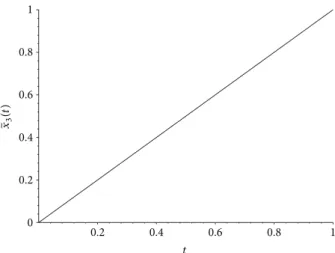
𝑉_𝑘(0) = 0, 𝑘 = 2, 3, . . . , 𝑁. (52) Thus, we get the approximated system of ordinary differential equations [𝐴 (𝛼 (𝑡) , 𝑁) 𝑡−𝛼(𝑡)+ 1] 𝑥 (𝑡) + 𝐵 (𝛼 (𝑡) , 𝑁) 𝑡1−𝛼(𝑡)𝑥(1)(𝑡) +∑𝑁 𝑘=2𝐶 (𝛼 (𝑡) , 𝑘) 𝑡 1−𝑘−𝛼(𝑡)_𝑉 𝑘(𝑡) = 1 Γ ((7 − 𝑡) /4)𝑡(3−𝑡)/4+ 𝑡, 𝑉_𝑘(1)(𝑡) = (𝑘 − 1) 𝑡𝑘−2𝑥 (𝑡) , 𝑘 = 2, 3, . . . , 𝑁, 𝑥 (0) = 0, 𝑉_𝑘(0) = 0, 𝑘 = 2, 3, . . . , 𝑁. (53) Now we apply any standard technique to solve the system of ordinary differential equations (53). We used the command dsolve of Maple. In Figure 4 we find the graph of the approximatioñ𝑥₃(𝑡) to the solution of problem (49), obtained by solving (53) with𝑁 = 3.Table 1 gives some numerical values of such approximation, illustrating numerically the fact that the approximatioñ𝑥₃(𝑡) is already very close to the exact solution𝑥(𝑡) = 𝑡 of (49). In fact the plot of ̃𝑥₃(𝑡) in Figure 4is visually indistinguishable from the plot of𝑥(𝑡) = 𝑡.

4.3. Fractional Variational Calculus of Variable Order. We

now exemplify how the expansions obtained inSection 3are useful to approximate solutions of fractional problems of the calculus of variations [21]. The fractional variational calculus of variable order is a recent subject under strong current development [15,16,22,23]. So far, only analytical methods to solve fractional problems of the calculus of variations of variable order have been developed in the literature, which consist in the solution of fractional Euler-Lagrange differential equations of variable order [15, 16, 22, 23]. In most cases, however, to solve analytically such fractional differential equations is extremely hard or even impossible, so numerical/approximating methods are needed. Our results

0.2 0.4 0.6 0.8 1 t 0 0.2 0.4 0.6 0.8 1 ̃x(t3 )

Figure 4: Approximatioñ𝑥3(𝑡) to the exact solution 𝑥(𝑡) = 𝑡 of the

fractional differential equation (49), obtained from the application

ofTheorem 7, that is, obtained by solving (53) with𝑁 = 3.

provide two approaches to this issue. The first was already illustrated inSection 4.2and consists in approximating the necessary optimality conditions proved in [15, 16, 22, 23], which are nothing else than fractional differential equations of variable order. The second approach is now considered. Similar to Section 4.2, the main idea here is to replace the fractional operators of variable order that appear in the formulation of the variational problem by the corresponding expansion of Section 3, which involves only integer-order derivatives. By doing it, we reduce the original problem to a classical optimal control problem, whose extremals are found by applying the celebrated Pontryagin maximum principle [24]. We illustrate this method with a concrete example. Consider the functional

𝐽 (𝑥) = ∫1 0 [0D 𝛼(𝑡) 𝑡 𝑥(𝑡) − _{Γ((7 − 𝑡)/4)}1 𝑡(3−𝑡)/4] 2 𝑑𝑡, (54) with fractional order𝛼(𝑡) = (𝑡+1)/4, subject to the boundary conditions

𝑥 (0) = 0, 𝑥 (1) = 1. (55) Since𝐽(𝑥) ≥ 0 for any admissible function 𝑥 and taking 𝑥(𝑡) = 𝑡, which satisfies the given boundary conditions (55), gives 𝐽(𝑥) = 0, we conclude that 𝑥 gives the global minimum to the fractional problem of the calculus of variations that consists in minimizing functional (54) subject to the boundary condi-tions (55). The numerical procedure is now explained. Since we have two boundary conditions, we replace ₀D𝛼(𝑡)_𝑡 𝑥(𝑡) by the expansion given inTheorem 7with𝑛 = 1 and a variable size𝑁 ≥ 2. The approximation becomes

0D𝛼(𝑡)𝑡 𝑥 (𝑡) ≈ 𝐴 (𝛼 (𝑡) , 𝑁) 𝑡−𝛼(𝑡)𝑥 (𝑡) + 𝐵 (𝛼 (𝑡) , 𝑁) 𝑡1−𝛼(𝑡)𝑥(1)(𝑡) +∑𝑁 𝑘=2𝐶 (𝛼 (𝑡) , 𝑘) 𝑡 1−𝑘−𝛼(𝑡)_𝑉 𝑘(𝑡) . (56)

(9)

Table 1: Some numerical values of the solutioñ𝑥3(𝑡) of (53) with𝑁 = 3, very close to the values of the solution 𝑥(𝑡) = 𝑡 of the fractional differential equation of variable order (49).

𝑡 0.2 0.4 0.6 0.8 1

̃𝑥3(𝑡) 0.20000002056 0.40000004031 0.60000009441 0.80000002622 1.0000001591

Using (56), we approximate the initial problem (54)-(55) by the following one: to minimize

̃𝐽(𝑥) = ∫1 0 [𝐴 (𝛼 (𝑡) , 𝑁) 𝑡 −𝛼(𝑡)_{𝑥 (𝑡)} + 𝐵 (𝛼 (𝑡) , 𝑁) 𝑡1−𝛼(𝑡)_𝑥(1)_(𝑡) +∑𝑁 𝑘=2 𝐶 (𝛼 (𝑡) , 𝑘) 𝑡1−𝑘−𝛼(𝑡)𝑉_𝑘(𝑡) −_{Γ((7 − 𝑡)/4)}1 𝑡(3−𝑡)/4]2𝑑𝑡 (57) subject to 𝑉_𝑘(1)(𝑡) = (𝑘 − 1) 𝑡𝑘−2𝑥 (𝑡) , 𝑉𝑘(0) = 0, 𝑘 = 2, . . . , 𝑁, 𝑥 (0) = 0, 𝑥 (1) = 1, (58)

where𝛼(𝑡) = (𝑡 + 1)/4. This dynamic optimization problem has a system of ordinary differential equations as a constraint, so it is natural to solve it as an optimal control problem. For that, define the control𝑢 by

𝑢 (𝑡) = 𝐴 (𝛼 (𝑡) , 𝑁) 𝑡−𝛼(𝑡)𝑥 (𝑡) + 𝐵 (𝛼 (𝑡) , 𝑁) 𝑡1−𝛼(𝑡)𝑥(1)(𝑡) +∑𝑁 𝑘=2𝐶 (𝛼 (𝑡) , 𝑘) 𝑡 1−𝑘−𝛼(𝑡)_𝑉 𝑘(𝑡) . (59)

We then obtain the control system 𝑥(1)(𝑡) = 𝐵−1𝑡𝛼(𝑡)−1𝑢 (𝑡) − 𝐴𝐵−1𝑡−1𝑥 (𝑡)

−∑𝑁

𝑘=2

𝐵−1𝐶_𝑘𝑡−𝑘𝑉_𝑘(𝑡) := 𝑓 (𝑡, 𝑥 (𝑡) , 𝑢 (𝑡) , 𝑉 (𝑡)) , (60) where, for simplification,

𝐴 = 𝐴 (𝛼 (𝑡) , 𝑁) , 𝐵 = 𝐵 (𝛼 (𝑡) , 𝑁) , 𝐶𝑘= 𝐶 (𝛼 (𝑡) , 𝑘) ,

𝑉 (𝑡) = (𝑉2(𝑡) , . . . , 𝑉𝑁(𝑡)) .

(61)

In conclusion, we wish to minimize the functional ̃𝐽(𝑥, 𝑢, 𝑉) = ∫1 0 [𝑢(𝑡) − 1 Γ((7 − 𝑡)/4)𝑡(3−𝑡)/4] 2 𝑑𝑡 (62)

subject to the first-order dynamic constraints 𝑥(1)(𝑡) = 𝑓 (𝑡, 𝑥, 𝑢, 𝑉) ,

𝑉_𝑘(1)(𝑡) = (𝑘 − 1) 𝑡𝑘−2𝑥 (𝑡) , 𝑘 = 2, . . . , 𝑁, (63) and the boundary conditions

𝑥 (0) = 0, 𝑥 (1) = 1,

𝑉_𝑘(0) = 0, 𝑘 = 2, . . . , 𝑁.

(64)

In this case, the Hamiltonian is given by 𝐻 (𝑡, 𝑥, 𝑢, 𝑉, 𝜆) = [𝑢 − _{Γ((7 − 𝑡)/4)}1 𝑡(3−𝑡)/4]2

+ 𝜆₁𝑓 (𝑡, 𝑥, 𝑢, 𝑉) +∑𝑁

𝑘=2

𝜆_𝑘(𝑘 − 1) 𝑡𝑘−2𝑥 (65) with the adjoint vector𝜆 = (𝜆₁, 𝜆₂, . . . , 𝜆_𝑁) [24]. Following the classical optimal control approach of Pontryagin et al. [24], we have the following necessary optimality conditions:

𝜕𝐻 𝜕𝑢 = 0, 𝑥(1)= 𝜕𝐻 𝜕𝜆₁, 𝑉_𝑝(1)= 𝜕𝐻 𝜕𝜆_𝑝, 𝜆(1)1 = −𝜕𝐻_𝜕𝑥, 𝜆(1)_𝑝 = −_𝜕𝑉𝜕𝐻 𝑝. (66)

That is, we need to solve the system of differential equations 𝑥(1)(𝑡) = 𝐵−1 Γ ((7 − 𝑡) /4) − 1 2𝐵−2𝑡2𝛼(𝑡)−2𝜆1(𝑡) − 𝐴𝐵−1_𝑡−1_{𝑥 (𝑡) −}_∑𝑁 𝑘=2 𝐵−1_𝐶 𝑘𝑡−𝑘𝑉𝑘(𝑡) , 𝑉(1) 𝑘 (𝑡) = (𝑘 − 1) 𝑡𝑘−2𝑥 (𝑡) , 𝑘 = 2, . . . , 𝑁, 𝜆(1) 1 (𝑡) = 𝐴𝐵−1𝑡−1𝜆1− 𝑁 ∑ 𝑘=2 (𝑘 − 1) 𝑡𝑘−2𝜆_𝑘(𝑡) , 𝜆(1) 𝑘 (𝑡) = 𝐵−1𝐶𝑘𝑡−𝑘𝜆1, 𝑘 = 2, . . . , 𝑁, (67)

(10)

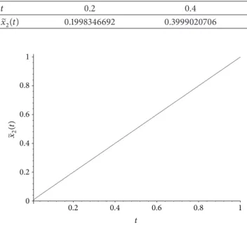
Table 2: Some numerical values of the solutioñ𝑥2(𝑡) of (67)-(68) with𝑁 = 2, close to the values of the global minimizer 𝑥(𝑡) = 𝑡 of the fractional variational problem of variable order (54)-(55).

𝑡 0.2 0.4 0.6 0.8 1 ̃𝑥2(𝑡) 0.1998346692 0.3999020706 0.5999392936 0.7999708526 1.0000000000 0.2 0.4 0.6 0.8 1 t 0 0.2 0.4 0.6 0.8 1 ̃x2 (t )

Figure 5: Approximatioñ𝑥2(𝑡) to the exact solution 𝑥(𝑡) = 𝑡 of the

fractional problem of the calculus of variations (54)-(55), obtained

from the application of Theorem 7 and the classical Pontryagin

maximum principle, that is, obtained by solving (67)-(68) with𝑁 =

2.

subject to the boundary conditions 𝑥 (0) = 0,

𝑉_𝑘(0) = 0, 𝑘 = 2, . . . , 𝑁, 𝑥 (1) = 1,

𝜆_𝑘(1) = 0, 𝑘 = 2, . . . , 𝑁.

(68)

Figure 5plots the numerical approximation ̃𝑥₂(𝑡) to the global minimizer𝑥(𝑡) = 𝑡 of the variable order fractional problem of the calculus of variations (54)-(55), obtained by solving (67)-(68) with 𝑁 = 2. The approximation ̃𝑥₂(𝑡) is already visually indistinguishable from the exact solution 𝑥(𝑡) = 𝑡 , and we do not increase the value of 𝑁. The effectiveness of our approach is also illustrated inTable 2, where some numerical values of the approximatioñ𝑥₂(𝑡) are given.

Acknowledgments

This work is supported by FEDER Funds through COMPETE—Operational Programme Factors of Com-petitiveness (“Programa Operacional Factores de Compet-itividade”) and by Portuguese Funds through the Center for

Research and Development in Mathematics and Applications

(University of Aveiro) and the Portuguese Foundation for Science and Technology (“FCT—Fundação para a Ciência e a Tecnologia”), within Project PEst-C/MAT/UI4106/2011 with COMPETE no. FCOMP-01-0124-FEDER-022690. Delfim F.M. Torres was also supported by EU Funding under the

7th Framework Programme FP7-PEOPLE-2010-ITN, Grant Agreement no. 264735-SADCO.

References

[1] M. Dalir and M. Bashour, “Applications of fractional calculus,” Applied Mathematical Sciences, vol. 4, no. 21–24, pp. 1021–1032, 2010.

[2] J. A. Tenreiro Machado, M. F. Silva, R. S. Barbosa et al., “Some applications of fractional calculus in engineering,” Mathemat-ical Problems in Engineering, vol. 2010, Article ID 639801, 34 pages, 2010.

[3] S. G. Samko and B. Ross, “Integration and differentiation to a variable fractional order,” Integral Transforms and Special Functions, vol. 1, no. 4, pp. 277–300, 1993.

[4] S. G. Samko, “Fractional integration and differentiation of variable order,” Analysis Mathematica, vol. 21, no. 3, pp. 213–236, 1995.

[5] A. Almeida and S. Samko, “Fractional and hypersingular oper-ators in variable exponent spaces on metric measure spaces,” Mediterranean Journal of Mathematics, vol. 6, no. 2, pp. 215–232, 2009.

[6] C. F. M. Coimbra, “Mechanics with variable-order differential operators,” Annalen der Physik (Leipzig), vol. 12, no. 11-12, pp. 692–703, 2003.

[7] C. M. Soon, C. F. M. Coimbra, and M. H. Kobayashi, “The variable viscoelasticity oscillator,” Annalen der Physik (Leipzig), vol. 14, no. 6, pp. 378–389, 2005.

[8] G. Diaz and C. F. M. Coimbra, “Nonlinear dynamics and control of a variable order oscillator with application to the van der Pol equation,” Nonlinear Dynamics, vol. 56, no. 1-2, pp. 145–157, 2009.

[9] C. F. Lorenzo and T. T. Hartley, “Variable order and distributed order fractional operators,” Nonlinear Dynamics, vol. 29, no. 1– 4, pp. 57–98, 2002.

[10] L. E. S. Ramirez and C. F. M. Coimbra, “On the selection and meaning of variable order operators for dynamic modeling,” International Journal of Differential Equations, vol. 2010, Article ID 846107, 16 pages, 2010.

[11] L. E. S. Ramirez and C. F. M. Coimbra, “On the variable order dynamics of the nonlinear wake caused by a sedimenting particle,” Physica D, vol. 240, no. 13, pp. 1111–1118, 2011. [12] S. Ma, Y. Xu, and W. Yue, “Numerical solutions of a

variable-order fractional financial system,” Journal of Applied Mathemat-ics, vol. 2012, Article ID 417942, 14 pages, 2012.

[13] D. Val´erio and J. S´a Da Costa, “Variable-order fractional deriva-tives and their numerical approximations,” Signal Processing, vol. 91, no. 3, pp. 470–483, 2011.

[14] P. Zhuang, F. Liu, V. Anh, and I. Turner, “Numerical methods for the variable-order fractional advection-diffusion equation with a nonlinear source term,” SIAM Journal on Numerical Analysis, vol. 47, no. 3, pp. 1760–1781, 2009.

[15] T. Odzijewicz, A. B. Malinowska, and D. F. M. Torres, “Frac-tional varia“Frac-tional calculus of variable order,” in Advances in

(11)

Harmonic Analysis and Operator Theory, the Stefan Samko Anniversary Volume, A. Almeida, L. Castro, and F. O. Speck, Eds., vol. 229 of Operator Theory: Advances and Applications, pp. 291–301, Springer, 2013.

[16] T. Odzijewicz, A. B. Malinowska, and D. F. M. Torres, “A gener-alized fractional calculus of variations,” Control and Cybernetics, vol. 42, no. 2, pp. 443–458, 2013.

[17] S. G. Samko, A. A. Kilbas, and O. I. Marichev, Fractional Integrals and Derivatives, Gordon and Breach, Yverdon, Switzer-land, 1993.

[18] S. Pooseh, R. Almeida, and D. F. M. Torres, “Numerical approximations of fractional derivatives with applications,” Asian Journal of Control, vol. 15, no. 3, pp. 698–712, 2013. [19] T. M. Atanackovic, M. Janev, S. Pilipovic, and D. Zorica, “An

expansion formula for fractional derivatives of variable order,” Central European Journal of Physics, 2013.

[20] S. Pooseh, R. Almeida, and D. F. M. Torres, “Approximation of fractional integrals by means of derivatives,” Computers & Mathematics with Applications, vol. 64, no. 10, pp. 3090–3100, 2012.

[21] A. B. Malinowska and D. F. M. Torres, Introduction to the Frac-tional Calculus of Variations, Imperial College Press, London, UK, 2012.

[22] T. Odzijewicz, A. B. Malinowska, and D. F. M. Torres, “Variable order fractional variational calculus for double integrals,” in Proceedings of the 51st IEEE Conference on Decision and Control, no. 6426489, pp. 6873–6878, Maui, Hawaii, USA, December 2012, Article 6426489.

[23] T. Odzijewicz, A. B. Malinowska, and D. F. M. Torres, “Noether’s theorem for fractional variational problems of variable order,” Central European Journal of Physics, vol. 11, no. 6, pp. 691–701, 2013.

[24] L. S. Pontryagin, V. G. Boltyanskii, R. V. Gamkrelidze, and E. F. Mishchenko, The Mathematical Theory of Optimal Processes, Interscience, John Wiley & Sons, New York, NY, USA, 1962, edited by L. W. Neustadt.

(12)

Submit your manuscripts at

http://www.hindawi.com

Operations

Research

Advances in

Hindawi Publishing Corporation

http://www.hindawi.com Volume 2013

Mathematical Problems in Engineering

Abstract and Applied Analysis Hindawi Publishing Corporation

ISRN

Applied Mathematics

International Journal of

Combinatorics

Journal of Function Spaces and Applications International Journal of Mathematics and Mathematical Sciences

Hindawi Publishing Corporation http://www.hindawi.com Volume 2013

ISRN

Geometry

Discrete Dynamics in Nature and Society

http://www.hindawi.com Volume 2013 Hindawi Publishing Corporation

Advances in

Mathematical Physics

ISRN

Algebra

Probability

and

Statistics

Journal of

ISRN

Mathematical Analysis

Journal of

Applied Mathematics

Sciences

Stochastic Analysis

International Journal of Hindawi Publishing Corporation

http://www.hindawi.com Volume 2013 Hindawi Publishing Corporation

The Scientific

World Journal

http://www.hindawi.com Volume 2013 ISRN

Discrete Mathematics

Hindawi Publishing Corporation http://www.hindawi.com

Differential Equations International Journal of