ACTA IMEKO
July 2012, Volume 1, Number 1, 19‐25 www.imeko.orgGene expression programming and genetic algorithms in
impedance circuit identification
Fernando M. Janeiro
1, Pedro M. Ramos
21 Instituto de Telecomunicações and Universidade de Évora, Largo dos Colegiais 2, 7004‐516 Évora, Portugal 2 Instituto de Telecomunicações and Instituto Superior Técnico/Universidade Técnica de Lisboa, Av. Rovisco Pais 1, 1049‐001 Lisbon,Portugal Keywords: Impedance spectroscopy; circuit topology identification; genetic algorithms; gene expression programming Citation: Fernando M. Janeiro, Pedro M. Ramos, Gene expression programming and genetic algorithms in impedance circuit identification, Acta IMEKO, vol. 1, no. 1, article 7, July 2012, identifier: IMEKO‐ACTA‐01(2012)‐01‐07 Editor: Paul Regtien, Measurement Science Consultancy, The Netherlands Received January 3rd , 2012; In final form May 21st , 2012; Published July 2012 Copyright: © 2012 IMEKO. This is an open‐access article distributed under the terms of the Creative Commons Attribution 3.0 License, which permits unrestricted use, distribution, and reproduction in any medium, provided the original author and source are credited Funding: FCT project PEst‐OE/EEI/LA0008/2011 Corresponding author: Fernando M. Janeiro, e‐mail: fmtj@uevora.pt 1. INTRODUCTION
Impedance spectroscopy [1] is used in different fields ranging from biomedical applications [2] to electrochemical applications such as the study of fuel cells [3]. Other applications include monitoring of anti-corrosion coatings [4] and sensor modelling, for example, of a humidity sensor [5]. The first step in performing impedance spectroscopy consists on obtaining the impedance spectral response [6]. This can be accomplished for example using an impedance vector-analyser or through a two-channel data acquisition system where a sine-fitting algorithm [7] is used to extract the impedance magnitude and phase [8]. An improved version of the basic sine-fitting algorithm, called 7-parameter sine-fitting [9], that is well suited as a digital signal processing algorithm to estimate the impedance parameters has been proposed.
Usually, to fit the acquired spectral data, some knowledge of the underlying processes is needed to suitably choose a circuit topology that models the process under study. With a known circuit topology, the Complex Non-Linear Least Squares (CNLS) method can be used to obtain the circuit parameters of the chosen model [10]. The CNLS implemented in [11] is based on the Levenberg-Marquardt algorithm and requires the input of the starting search values and then, it will efficiently converge to the local minima near this set of initial parameters.
To avoid the convergence to the local minima, a new approach [12] based on a hybrid genetic algorithm (GA) [13] was proposed. This approach has been used to characterize a viscosity measurement system [14].
Gene Expression Programming (GEP) [15] was proposed as a method to search for suitable circuit topologies without any prior knowledge of the equivalent circuit [16]. In that work, a basic genetic algorithm was used to estimate the values of the circuit components. A different approach, based on GEP and cultural algorithms, was used for the modelling of electrochemical phenomena in [17].
In this work, which is an extended version of [18], GEP is interleaved with an improved version of the genetic algorithm to identify the circuit topology and circuit component values. A more effective fitness function, which works well for impedance responses that include resonances, is also used in this paper. In order to make the numerical simulations more realistic, measurement uncertainty is included for the magnitude and phase impedance data. Further validation of the algorithm is performed by its application to impedance measurements performed on a circuit that models the humidity sensor presented in [19] and on the viscosity sensor used in [14].
Impedance circuit identification through spectroscopy is often used to characterize sensors. When the circuit topology is known, it has been shown that the component values can be obtained by genetic algorithms. Also, gene expression programming can be used to search for an adequate circuit topology. In this paper, an improved version of the impedance circuit identification based on gene expression programming and hybrid genetic algorithm is presented to both identify the circuit and estimate its parameters. Simulation results are used to validate the proposed algorithm in different situations. Further validation is presented from measurements on a circuit that models a humidity sensor and also from measurements on a viscosity sensor.
2. EVOLUTIONARY ALGORITHMS
Equivalent circuit identification from impedance spectroscopy involves identifying the circuit topology and then optimizing the values of each component in that circuit. This is accomplished in two interleaved steps; (i) a GEP implementation is used to identify potential circuit network topologies that can model the measured impedance; (ii) a hybrid genetic algorithm is applied to each topology to obtain the values of the components that minimize the cost function. In the next subsections these two algorithms are described.
2.1. Equivalent Impedance Parameters Estimation
For a given circuit topology, the optimization of the component values is performed using a hybrid genetic algorithm [12]. Initially, a population of M chromosomes is created where each chromosome is composed by the values of each component in the current circuit topology. The fitness of each chromosome is usually evaluated through the cost function
2 2 1 1 P i est i i i Z Z P Z
(1)where Z
is the measured impedance at angular ifrequencies i 2 fi, Zest
is the estimated impedance iobtained with the component values in the chromosome and P is the number of measurement frequencies. However, in circuits that exhibit resonance-like behaviour, the frequency points in the resonance region could have little weight in the final value of the cost function. This led to having good candidate circuits being discarded by the genetic algorithm. To tackle this issue, a different cost function that does not suffer from these problems was used
2 2 1 1 P i est i i est i Z Z P Z
. (2)With this cost function, the absolute error of the impedance estimation is normalized by the estimated impedance, therefore giving more weight to frequency points in the resonance region. If information regarding the quality of each measurement value is available (e.g., experimental standard deviation), weights can be used in (2) to make sure that the fitting algorithm is more influenced by the measurement values with reduced uncertainty. The fitness of each chromosome is used to evolve the population based on survival of the fittest. Just like in a biological population, there is reproduction and mutation. In reproduction, pairs of chromosomes are randomly chosen using a biased roulette wheel selection scheme where the fittest elements have a higher probability of being chosen to reproduce. Each pair of chromosomes may create two offspring through the crossover operation or move directly to the next generation. In mutation, randomly chosen positions on some chromosomes are replaced by random generated values. Mutation is vital to maintain population diversity and escape local minima of the cost function.
Traditional minimum search algorithms, such as the Levenberg-Marquardt algorithm and the Gauss-Newton method, are very sensitive to the starting search values and are not able to escape local minimums of the cost function. However, genetic algorithms are very efficient in finding the
region of the absolute minimum of multi-dimensional cost functions even when the search space is vast and local minima are present nearby [20]. Although genetic algorithms are suitable to find the global minimum of the cost function, they take a long time to converge to the actual minimum. Therefore, a Gauss-Newton method is applied using the final results of the genetic algorithm as starting values for the Gauss-Newton method.
2.2. Impedance Network Topology Identification
The identification of the equivalent impedance network topology is performed using GEP. Each candidate circuit is expressed as a gene which contains components (R, L and C) and operators (series and parallel). The gene is composed of a head of size h and a tail of size t, with t h 1. The head may contain components and operators while the tail is comprised only of components. This is fundamental to the operation of GEP since it guarantees a valid circuit topology under all circumstances.
Each gene is converted into a binary tree by filling it in a breadth-first fashion as proposed in [15]. This tree can then be recursively run to obtain the equivalent circuit. Breadth-first traversal of the tree, also known as width first, consists on filling the tree from left to right and top to bottom. When there are no more node positions to fill in the current level of the tree, the tree filling starts from left to right in the next lower level.
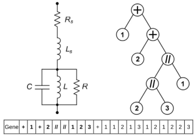
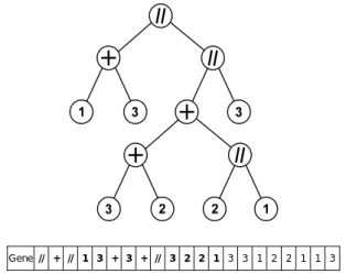
In this implementation of GEP, the binary tree is completely bypassed and is only used to help visualize the circuit topology. As an example, Figure 1 shows an electric circuit that will be used as test impedance in the numerical results. The GEP gene that codes this circuit is presented along with the corresponding binary tree. The numbers in the tree leafs correspond to the type of component R, L or C for 1, 2 or 3, respectively. Notice that, in the 21 long gene, only the first 9 elements (shown in bold) correspond to the described circuit. The remaining elements are also part of the gene but do not define the circuit. Also noticeable is that the last 11 elements (the tail) are all components.
Initially, a population of N circuit topologies is randomly created according to the previously described rules. The hybrid genetic algorithm is then executed for each candidate topology gene to optimize its component values and obtain its fitness. Afterwards, this population is used to create a new generation of circuit topologies trough the GEP operations: replication, mutation, transposition and recombination [15]. The new
Gene + 1 + 2 // // 1 2 3 + 1 1 2 1 3 1 2 1 2 2 3
Figure 1. Example of circuit topology and corresponding binary tree along with coding gene for GEP with h + t = 21. The coding region is shown in bold and ends at position 9.
generation is again evaluated by the hybrid genetic algorithm and the process repeats itself until a valid circuit is found (i.e., until its fitness is better than a predefined threshold) or the maximum number of generations is reached, in which case the algorithm failed to find a suitable circuit.
In the creation of a new generation, GEP operators are applied sequentially. The replication operator creates an intermediate population by choosing, based on a biased roulette wheel selection scheme, which genes survive from the original population. The fittest elements have a higher probability of being chosen and so multiple copies of them may appear in this intermediate population. Genes with low fitness may not be chosen at all.
Mutation is applied to the intermediate population by changing the value of a random position inside some randomly chosen genes. If the position is inside the head it can be mutated into a circuit component or an operation, while if it is in the tail it is restricted to mutate only into a circuit component. This is mandatory to maintain the structural integrity of the genes.
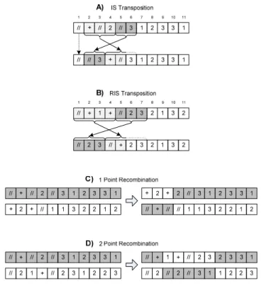
Insert sequence transposition (IS transposition) is then applied to some randomly chosen genes of the population that resulted from the mutation. In each chosen gene, a sequence of random length is transposed to any position in the head except to the root. An example is shown in Figure 2A where, for the sake of simplicity, a smaller gene with h + t = 11 is used. The insertion sequence has length 2 and starts on position 5. The sequence was inserted at the randomly chosen position 2 and the head elements below the insertion point are moved downstream inside the head. However, to maintain gene integrity, the tail remains untouched and the last two positions of the original head are discarded. This operator creates a new intermediate population to which root insertion sequence transposition is applied.
Root insertion sequence transposition (RIS transposition) is very similar to the previous operator, except that the insertion point is always the root. The insertion sequence is also of
random length but must start with an operation. Figure 2B illustrates this behaviour, where the insertion sequence has length 3 and starts in position 5. It is inserted at the root and the remaining head elements are moved downstream, with the last 3 elements being discarded in order to maintain the original tail.
The next operation is the 1 point recombination. Two genes and a crossover point are randomly chosen. Then, the two genes exchange part of their information as shown in Figure 2C. In the example, the crossover point is 3 and therefore positions 1 to 3 are exchanged between the two genes. The last operation is the 2 point recombination, where 2 crossover points are chosen. In the example presented in Figure 2D, positions 3 to 7 are exchanged between the two genes. In recombination, the integrity of the gene structure is always assured.
At the end of this sequence of operations, a new generation of candidate circuits has been created. Also, due to the use of elitism, a copy of the best circuit topology is always included in the new population. These operations can profoundly change the population genes and, although the genes are of fixed length, their circuit coding region varies, resulting in trees of different sizes and complexity. This means that GEP can add branches to the circuit or eliminate them, while searching for the circuit that best fits the measured data. Before applying the GA, a basic circuit simplify algorithm searches the tree for operations that have, on the two leafs, identical type components. These correspond for example to two identical type components in series or in parallel and can be replaced by a single component.
3. NUMERICAL RESULTS
In this section, the circuit in Figure 1 is used to test the proposed algorithm and the threshold to stop the algorithm is set at 0.0002%. The spectral response of this impedance with Rs = 10 , R = 1000 , Ls = L = 1 mH and C = 1 F was
calculated for P = 100 linearly spaced frequency points in the 100 Hz to 10 kHz range and random errors were included in the data to simulate real measurement conditions, with an uncertainty of 0.08% in the impedance magnitude and 0.05º in its phase. The encoding gene chosen by the algorithm is presented in Figure 3, along with its corresponding binary tree. The resulting equivalent circuit is presented in Figure 4 with the estimated component values. The corresponding frequency responses are shown in Figure 5.
Although the equivalent circuit does not have the same topology as the original impedance circuit, the effect of the
Figure 2. Examples of the main GEP operations on genes with h + t = 11.
Gene + // // + 3 + // 1 2 2 1 3 2 2 2 1 3 2 2 2 2
Figure 3. Encoding gene (in bold) and corresponding binary tree obtained by GEP and hybrid genetic algorithm for the impedance in Figure 1 with
capacitor in the first parallel circuit (the 4.934 pF capacitor) and of the inductor in series with the resistance in the second part of the circuit (the 900.3 H inductor) are negligible in the frequency range under study, as can be seen in Figure 5 where the spectral response of the two circuits is shown. Different runs of the algorithm yield different equivalent circuits, but always in good agreement with the spectral response of the original circuit. It should be noted that, in many applications, an equivalent circuit with physical meaning is needed, which is a requirement that is currently not satisfied by the GEP and GA algorithm.
In Figure 6, the errors of the fit for this situation are presented. In Figure 6A, the difference between the magnitudes of the simulated and estimated impedance are shown, while in Figure 6B, the difference of the simulated and estimated phase are depicted. Note that, the cost function must combine the magnitude and phase information to estimate a single value that quantifies the fit of each circuit and corresponding estimated circuit parameters. So, in Figure 6C the magnitude of the difference between the two impedances (corresponding to the distance between the two complex numbers that represent the estimated and simulated impedances) is shown. In order to ensure that higher impedance magnitudes that occur at certain frequencies don’t overly influence the cost function solely due to their higher magnitude, the magnitude of the difference between the estimated and simulated impedance are normalized by the estimated impedance magnitude. This corresponds to each frequency point in cost function (2) and is shown, for this case, in Figure 6D. The average of the squared values represented in Figure 6D corresponds to the fitting error. In this situation 1.2 10 6 0.00012%.
Since it is not realistic to measure impedance values for 100 different frequencies, the usefulness of the proposed algorithm depends on its performance with fewer measurements. In Figures 7, 8 and 9 the results obtained with only 10 frequency points are presented.
The circuit topology is quite similar to the original circuit with just the addition of a capacitor in parallel with the correct circuit.
As can be seen in Figure 8, the magnitude and phase responses of the estimated circuit closely match the original circuit frequency responses. Therefore, the extra capacitor relative to the original circuit (the 14.26 pF capacitor), has a negligible effect on the overall impedance at the frequency range under study. Note that, even without any measured point in the resonance region, the algorithm still finds a correct equivalent circuit. Figure 9 presents the normalized impedance errors for this case, corresponding to a fitting error of
0.00013%
.
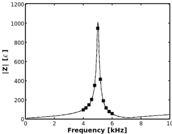
In the third analysis of the performance of the proposed algorithm, the circuit of Figure 1 is considered, but the simulated impedance values are narrowly centred near the resonance. In this case, 11 frequency points are used in the 4 kHz to 6 kHz range. In Figure 10, the magnitude frequency
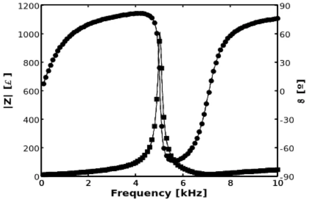
0 2 4 6 8 10 0 200 400 600 800 1000 1200 Frequency [kHz] |Z | [ ] 0 2 4 6 8 10-90 -60 -30 0 30 60 90 [º ] Figure 5. Impedance magnitude and phase of the circuit in Figure 1 (lines), estimated impedance magnitude and phase corresponding to the circuit in Figure 4 (dashed lines overlapped with lines) and frequency points used for estimation (squares for magnitude and circles for phase). 0 2 4 6 8 10 -0.3 -0.2 -0.1 0 0.1 0.2 0.3 Frequency [kHz] |Zm |-|Z | [ ] 0 2 4 6 8 10 -0.2 -0.1 0 0.1 0.2 Frequency [kHz] m - [º] 0 2 4 6 8 10 0 0.1 0.2 0.3 0.4 Frequency [kHz] |Zm -Z| [ ] 0 2 4 6 8 10 0 1 2 3x 10 -3 Frequency [kHz] |Z m -Z|/| Z | A C B D Figure 6. Four representations of the fitting errors.
Figure 4. Circuit topology and component values corresponding to the binary tree shown in Figure 3.
response of the original circuit and that of the estimated circuit are compared with the values considered for the circuit estimation. Although the frequency points are very close to the resonance, the magnitude estimation is quite good even in the complete frequency range represented.
Figure 11 shows the results obtained for the phase. In this case, the overall estimation is quite good near the resonance but nearer the edges of the complete frequency range, there are some small noticeable differences. In this case, the error of the fit is 0.00014% (Figure 12).
4. EXPERIMENTAL RESULTS
The next step in testing the developed algorithm is to evaluate its performance when applied to real measured data. Measurements were performed in a circuit that models a humidity sensor [19] and in a previously analysed viscosity sensor [14].
4.1. Humidity Sensor Circuit Model
The circuit that models the humidity sensor is represented in Figure 13. The component values of the equivalent circuit of the sensor change with relative humidity and the case corresponding to a relative humidity of 54% is considered. The component values are presented in Table 1.
The circuit in Figure 13 with the component values shown in Table 1 was assembled and its spectral response was measured for P = 11 logarithmic spaced frequency points in the 1 Hz to 100 kHz range. The proposed algorithm was then applied to these measurements to find the equivalent circuit and
Figure 7. Circuit topology and component values obtained with the proposed algorithm for 10 different frequencies in the 100 Hz to 10 kHz range. 0 2 4 6 8 10 0 200 400 600 800 1000 1200 Frequency [kHz] |Z | [ ] 0 2 4 6 8 10-90 -60 -30 0 30 60 90 [ º] Figure 8. Impedance magnitude and phase of the circuit in Figure 1 (lines), estimated impedance magnitude and phase corresponding to the circuit in Figure 7 (dashed lines overlapped with lines) and frequency points used for estimation (squares for magnitude and circles for phase). 0 2 4 6 8 10 0 1 2 3x 10 -3 Frequency [kHz] |Zm -Z |/ |Z | Figure 9. Normalized impedance errors for 10 linearly spaced frequencies in the 100 Hz to 10 kHz range. 0 2 4 6 8 10 0 200 400 600 800 1000 1200 Frequency [kHz] |Z | [ ] Figure 10. Impedance magnitude of the circuit in Figure 1 (line), estimated impedance magnitude corresponding to the original circuit (dashed line overlapped with line) and frequency points used for the estimation (squares) in the 4 kHz to 6 kHz range. 0 2 4 6 8 10 -90 -60 -30 0 30 60 90 Frequency [kHz] [º]
Figure 11. Impedance phase of the circuit in Figure 1 (line), estimated impedance phase corresponding to the original circuit (dashed line) and frequency points used for the estimation (circles) in the 4 kHz to 6 kHz range. 4 5 6 0 0.5 1 1.5 2x 10 -3 Frequency [kHz] |Zm -Z |/ |Z | Figure 12. Normalized impedance errors for 11 linearly spaced frequencies in the 4 kHz to 6 kHz range.
respective component values. Figure 14 shows an example of the encoding gene and the respective binary tree that was found by the algorithm. The corresponding equivalent circuit with the component values is presented in Figure 15.
Although different runs of the algorithm on the measured data yield different equivalent circuits that do not resemble the original circuit topology shown in Figure 13, the spectral response of the resulting circuit closely matches the measurements performed on the original circuit, as shown in Figure 16. Thus, it is possible to conclude that the circuit in Figure 15 is equivalent, at least in the measured frequency range, to the original circuit although it might not be equivalent to the sensor equivalent circuit at different relative humidity values. The error of the fit is 0.032% (the threshold was set, in this case, to 0.035% due to noisy measurements).
4.2. Viscosity Sensor
The viscosity sensor consists on a vibrating wire cell whose resonance characteristics change with the viscosity of the liquid in which the wire is immersed and also on its temperature. From the measured frequency response of the sensor, it is possible to obtain its resonance characteristics and in turn obtain the viscosity of the liquid. Further details on the working principle of this sensor can be found in [14].
The viscosity sensor wire was immersed in diisodecyl phthalate (DIDP) liquid at 15ºC. Its impedance was then measured for P = 21 frequency values in the range 500 Hz to 1.5 kHz. From the application of the GEP and the hybrid genetic algorithms resulted the equivalent circuit and respective component values presented in Figure 17.
The impedance frequency response of the equivalent circuit in Figure 17 is plotted in Figure 18 along with the 21 measured points. Both magnitude and phase are in close agreement with the measurements showing that, also in this case, the algorithm was successful in finding an equivalent circuit. The error of the fit is 0.00008%, while the threshold was set at 0.0001%.
5. CONCLUSIONS
In this paper, an improved version of impedance spectroscopy using evolutionary algorithms was presented, where GEP is used to evolve the target circuit topology and a hybrid genetic algorithm estimates the circuit component values. A detailed description of the GEP algorithm and operators is presented as well as a summary of the hybrid genetic algorithm.
Figure 13. Humidity sensor equivalent circuit. The component values change with relative humidity [19].
Gene // + // 1 3 + 3 + // 3 2 2 1 3 3 1 2 2 1 1 3
Figure 14. Example of encoding gene (in bold) and corresponding binary tree obtained by GEP and hybrid genetic algorithm for the measured spectral response of the sensor equivalent circuit with RH = 54%.
Table 1. Component values for the humidity sensor equivalent circuit at
RH = 54%. Component Value Rs 1.18 Rw 624.5 Rb 30 M Rp 120.97 k Cb 0.68 F Cp 2.32 F Cpw 5.87 nF 0.4183 F 0.1130 H 620.0 10.76 H 5.711 nF 1.746 M 0.1275 F
Figure 15. Circuit topology and component values corresponding to the binary tree shown in Figure 14. 10-2 100 102 102 103 104 105 106 Frequency [kHz] |Z| [ ] 10-3 10-2 10-1 100 101 10-902 -75 -60 -45 -30 -15 0 [º ] Figure 16. Estimated impedance magnitude and phase (lines) of the circuit in Figure 15 versus the measured impedance magnitude (squares) and phase (circles) of the circuit in Figure 13.
To improve the convergence properties of the algorithm, a different fitness function, which works well with impedance sweeps that include resonances, has been proposed. Numerical results show that even with measurement uncertainties and few frequency impedance measured values, the presented algorithm is capable of finding an equivalent circuit. The residual errors in the magnitude and phase of the estimated impedances were used to analyse the performance of the algorithm.
The algorithm was also applied to measurements of a circuit that models a humidity sensor at a specific relative humidity and to a viscosity sensor. In both cases it was found that different runs of the algorithm yield different equivalent circuits that nonetheless closely match the measured spectral responses. A method for further automatic simplification of the obtained circuits is currently under development.
ACKNOWLEDGEMENT
The authors would like to thank Prof. J. Fareleira and Prof. F. Caetano for the use of their viscosity sensor.
REFERENCES
[1] J.R. Macdonald, Impedance spectroscopy, Annals of Biomedical Engineering, 20, (1992), pp. 289-305.
[2] E. Katz, I. Willner, Probing biomolecular interactions at conductive and semiconductive surfaces by impedance spectroscopy: Routes to impedimetric immunosensors,
DNA-Sensors, and Enzyme Biosensors, Electroanalysis, 15, (2003), pp. 913–947.
[3] A.K. Manohar, O. Bretschger, K.H. Nealson, F. Mansfeld, The use of electrochemical impedance spectroscopy (EIS) in the evaluation of the electrochemical properties of a microbial fuel cell, Bioelectrochemistry, 72, (2008), pp. 149-154.
[4] J. Hoja, G. Lentka, Interface circuit for impedance sensors using two specialized single-chip microsystems, Sensors and Actuators A: Physical, 163, (2010), pp. 191-197.
[5] J. Hoja, G. Lentka, Method using bilinear transformation for measurement of impedance parameters of a multielement two-terminal network, IEEE Trans. Instrumen. Meas., 57, (2008), pp. 1670-1677.
[6] E. Barsoukov, J. Macdonald, Impedance spectroscopy theory, experiment, and applications, Wiley Interscience, Hoboken, 2005, ISBN 978-0-471-64749-2.
[7] IEEE Std. 1057-2007, IEEE standard for digitizing waveform records, The Institute of Electrical and Electronic Engineers, (2007), New York, December, E-ISBN: 0-7381-4543-2.
[8] P.M. Ramos, M.F. Silva, A.C. Serra, Low frequency impedance measurement using sine-fitting, Measurement, 35, (2004), pp. 89-96.
[9] P.M. Ramos, A.C. Serra, A new sine-fitting algorithm for accurate amplitude and phase measurements in two channel acquisition systems, Measurement, 41, (2008), pp. 135-143. [10] J.R. Macdonald, J.A. Garber, Analysis of impedance and
admittance data for solids and liquids, J. Electrochem. Soc., 124, (1977), pp. 1022-1030.
[11] R. Macdonald, LEVM/LEVMW Manual, Version 8.11, October 2011, available at www.jrossmacdonald.com/ levminfo.html. [12] F.M. Janeiro, P.M. Ramos, Application of genetic algorithms for
estimation of impedance parameters of two-terminal networks, I2MTC 09, Singapore, 2009, pp. 602-606.
[13] F.M. Janeiro, P.M. Ramos, Impedance measurements using genetic algorithms and multiharmonic signals, IEEE Trans. Instrumen. Meas., 58, (2009), pp. 383-388.
[14] F.M. Janeiro, J. Fareleira, J. Diogo, D. Máximo, P. M. Ramos, F. Caetano, Impedance spectroscopy of a vibrating wire for viscosity measurements, I2MTC 10, Austin, USA, 2010,
pp. 1067-1072.
[15] C. Ferreira, Gene expression programming in problem solving, 6th Online World Conference on Soft Computing in Industrial Applications, 2001.
[16] H. Cao, J. Yu, L. Kang, An evolutionary approach for modeling the equivalent circuit for electrochemical impedance spectroscopy, The 2003 Congress on Evolutionary Computation, Canberra, Australia, 2003, pp. 1819-1825.
[17] P. Arpaia, A cultural evolutionary programming approach to automatic analytical modeling of electrochemical phenomena through impedance spectroscopy, Meas. Sci. Technol., 20, (2009), pp. 1-10.
[18] F.M. Janeiro, P.M. Ramos, Impedance circuit identification through evolutionary algorithms, XVIII TC 4 IMEKO Symposium, Natal, Brazil, 2011.
[19] J.A. González, V. López, A. Bautista, E. Otero, X. R. Nóvoa, Characterization of porous aluminum oxide films from a.c. impedance measurements, J. Appl. Electrochem., 29, (1999), pp. 229-238.
[20] R.L. Haupt, S. E. Haupt, Practical genetic algorithms, Wiley-Interscience, Hoboken, 2004, ISBN 978-0-471-45565-3.