Interpretation of Searches for Supersymmetry with simplified Models

CERN-PH-EP/2012-351 2013/12/03

CMS-SUS-11-016

Interpretation of searches for supersymmetry with

simplified models

The CMS Collaboration

Abstract

The results of searches for supersymmetry by the CMS experiment are interpreted in the framework of simplified models. The results are based on data correspond-ing to an integrated luminosity of 4.73 to 4.98 fb−1. The data were collected at the LHC in proton–proton collisions at a center-of-mass energy of 7 TeV. This paper de-scribes the method of interpretation and provides upper limits on the product of the production cross section and branching fraction as a function of new particle masses for a number of simplified models. These limits and the corresponding experimen-tal acceptance calculations can be used to constrain other theoretical models and to compare different supersymmetry-inspired analyses.

Published in Physical Review D as doi:10.1103/PhysRevD.88.052017.

c

2013 CERN for the benefit of the CMS Collaboration. CC-BY-3.0 license

∗_{See Appendix A for the list of collaboration members}

1

Introduction

The results of searches for supersymmetry (SUSY) [1] at particle colliders are often used to test the validity of a few, specific, theoretical models. These models predict a large number of ex-perimental observables at hadron colliders as a function of a few theoretical parameters. Most of the SUSY analyses performed by the Compact Muon Solenoid (CMS) experiment present their results as an exclusion of a range of parameters for the constrained minimal supersym-metric standard model (CMSSM) [2–4]. However, the results of the SUSY analyses can be used to test a wide range of alternative models, since many SUSY and non-SUSY models predict a similar phenomenology. These similarities inspired the formulation of the simplified model framework for presenting experimental results [5–9]. Specific applications of these ideas have appeared in Refs. [10, 11].

A simplified model is defined by a set of hypothetical particles and a sequence of their produc-tion and decay. For each simplified model, values for the product of the experimental accep-tance and efficiency (A ×e) are calculated to translate a number of signal events into a signal

cross section. From this information, a 95% confidence level upper limit (UL) on the product of the cross section and branching fraction ([σ× B]_UL) is derived as a function of particle masses.

The simplified model framework can quantify the dependence of an experimental limit on the particle spectrum or a particular sequence of particle production and decay in a manner that is more general than the CMSSM. Furthermore, the values of[σ× B]_ULcan be compared with

theoretical predictions from a SUSY or non-SUSY model to determine whether the theory is compatible with data.

This paper collects and describes simplified model interpretations of a large number of SUSY-inspired analyses performed on data collected by the CMS collaboration in 2011 [12–26]. The simplified model framework was also applied by CMS to a limited number of analyses in 2010 [27]. The ATLAS collaboration has published similar interpretations [28–34].

The paper is organized as follows: Section 2 provides a brief description of the CMS analyses considered here; Section 3 describes simplified models; Section 4 demonstrates the calculation of the product of the experimental acceptance and efficiency and the upper limits on cross sections; Section 5 contains comparisons of the results for different simplified models and anal-yses; Section 6 contains a summary.

2

The CMS detector and analyses

The CMS detector consists of a silicon tracker, an electromagnetic calorimeter, and a hadronic calorimeter, all located within the field volume of a central solenoid magnet, and a muon-detection system located outside the magnet [35]. Information from these components is com-bined to define objects such as electrons, muons, photons, jets, jets identified as b jets (b-tagged jets), and missing transverse energy (E/ ). The exact definition of these objects depends on theT

specific analysis, and can be found in the analysis references. The data were collected by the CMS experiment at the Large Hadron Collider in proton-proton collisions at a center-of-mass energy of 7 TeV. Unless stated otherwise, the data corresponds to an integrated luminosity of 4.98±0.11 fb−1[36].

The descriptions of the analyses are categorized by the main features of the event selection. Detailed descriptions of these analyses can be found in the references [12–26]. The target of these analyses is a signal of the production of new, heavy particles that decay into standard model particles and stable, neutral particles that escape detection. The stable, neutral particles

can produce a signature of large E/ . The standard model also produces ET / in top quark, weakT

gauge boson, and heavy flavor production. Fluctuations in energy deposition in the detector can also produce significant E/ in quantum chromodynamics processes.T

All-Hadronic Events contain two or more high transverse momentum (pT) jets and significant

ET

/ . Events with isolated leptons are rejected to reduce backgrounds from tt, W, and Z bo-son production. A selection on kinematic discriminants is applied to reduce backgrounds containing E/ . The names of the discriminants label the analyses: αT T [12], 6HT+jets [13]

and MT2[14]. The αT[37] and MT2[38, 39] variables are both motivated by the kinematics

of new-particle pair production and decay into two visible systems of jets and a pair of invisible particles. The6HT+jets analysis, instead, uses a selection on the negative vector

sum (6HT) and the scalar sum (HT) of the transverse momentum of each jet. The MT2

analysis uses data corresponding to an integrated luminosity of 4.73±0.10 fb−1

The αT analysis mentioned above also categorizes events with one, two, or at least three

jets that satisfy a b-tagging requirement. The MT2b analysis modifies the MT2 selection

mentioned above and requires at least one b-tagged jet. The E/T+b analysis [15] follows a

similar strategy as the6HT+jets analysis, but selects events with one, two, or at least three

b-tagged jets.

Single Lepton + Jets Events are selected with one high-pT, isolated lepton (electron or muon),

jets, and significant E/ . Three analyses are considered in this paper [17]. The lepton spec-T

trum (e/µ LS) and lepton projection (e/µ LP) methods exploit the expected correlation between the lepton pT and E/ from W boson decays to separate a potential signal fromT

the main backgrounds of tt and W+jets production. The artificial neutral network (ANN) method applies an ANN that is based on event properties (jet multiplicity, HT, transverse

mass, and the azimuthal angular separation between the two highest-pT jets) to separate

backgrounds from the expectations of a CMSSM benchmark model.

Two other analyses [18] require also two or more b-tagged jets. In the first analysis (e/µ ≥ 2b+E/ ), the WT +, W−, and tt background distributions from simulation are

cor-rected to match the measured E/ spectrum at low HT T, and then the corrected prediction

is extrapolated to high HT and high E/ . A selection on ET / significance (YT MET) and HT is

used in the second analysis (e/µ ≥ 3b, YMET). The YMET variable is defined as the ratio

of E/ toT

√ HT.

Opposite-Sign Dileptons Events are selected with two leptons (electrons or muons) having

electric charge of the opposite sign (OS), jets, and significant E/ . In one (OS e/µT +E/ )T

analysis [21], a signal is defined as an excess of events at large values of E/ and HT T.

In a second (OS e/µ edge) analysis [21], a search is performed for a characteristic kine-matic edge in the dilepton mass distribution m`+<sub>`</sub>−. In these two analyses events with

an e+_e− _{or µ}+

µ− pair with invariant mass of the dilepton system between 76 GeV and

106 GeV or below 12 GeV are removed, in order to suppress Z/γ∗events, as well as low-mass dilepton resonances. A third analysis (OS e/µ ANN) [22] applies a selection on the output of an ANN that is based on seven kinematic variables constructed from leptons and jets, to discriminate the signal events from the background.

Two other analyses complementary focus directly on the two leptons from Z-boson decay by applying an invariant mass selection [25]. With this requirement, the main source of E/ arises from fluctuations in the measurement of jet energy. One analysis (ZT +E/ )T

determines this background from a control sample that differs only in the presence of a Z boson. A second analysis (JZB) applies a kinematic variable denoted JZB, which is

defined as the difference between the sum of the vector elements of the pTof the jets and

the pTof the boson candidate.

The last analysis in this group selects events consistent with a W boson decaying to jets produced in association with a Z boson decaying to leptons, and searches for an excess of events in the E/ distribution. This analysis is part of the combined lepton (comb. leptons)T

analysis [24] that targets a signal containing gauge boson pairs and E/ : WZ, ZZT +E/ .T

Same-Sign Dileptons Events are selected with two leptons (electrons or muons) having

elec-tric charge of the same sign (SS), and significant E/ . One analysis (SS e/µ) uses severalT

different selections on E/ and HT Tto suppress backgrounds [19]. A second analysis (SS+b)

requires at least one b-tagged jet [20]. A third analysis makes no requirements on jet activity. It limits backgrounds by applying more stringent lepton identification criteria. Results from this analysis are included in the combined lepton results [24].

Multileptons Events are selected containing at least three leptons. Selections are made on

the values of several event variables, including E/ , HT T, and the invariant mass of

lep-ton pairs [23, 24]. One analysis applies a veto on b-tagged jets to remove most of the tt background, and is included in the combined lepton results [24].

Photons Events are selected containing one photon, two jets, and E/ (γjjT +E/ ), or two photons,T

one jet, and E/ (γγjT +E/T)[26]. The requirement of a photon and E/ is sufficient to removeT

most backgrounds.

Inclusive The razor analysis integrates several event categories [16]. Events are required to

contain jets and zero, one, or two leptons (electrons and muons) with a further classifi-cation based on the presence of a b-tagged jet. The razor variable [40] is a ratio of a jet system mass to a transverse mass. The distribution in the razor variable is highly cor-related with the mass values of new particles for hypothesized signals but skewed to relatively smaller values for backgrounds. Values of the razor variable are chosen to re-duce backgrounds while accepting signal events in a similar manner as for the αT and

MT2 analyses. The razor analysis uses data corresponding to an integrated luminosity of

4.73±0.10 fb−1.

3

Simplified models

A simplified model is defined by a set of hypothetical particles and a sequence of their pro-duction and decay. In this paper, the selection of models is motivated by the particles and interactions of the CMSSM or models with generalized gauge mediation [41]. For convenience, the particle naming convention of the CMSSM is adopted, but none of the specific assumptions of the CMSSM are imposed. The CMSSM assumptions include relationships among the new particle masses, their production cross sections and distributions, and their decay modes and distributions. In the simplified models under consideration, only the production process for two primary particles is considered. Each primary particle can undergo a direct decay or a cascade decay through an intermediate new particle. Each particle decay chain ends with a neutral, undetected particle, denoted LSP (lightest supersymmetric particle) in text andχeLSPin equations.χeLSPcan represent a neutralino or gravitino LSP. The masses of the primary particle and the LSP are free parameters. When the model includes the cascade decay of a mother par-ticle (mother) to an intermediate parpar-ticle (int), the mass of the intermediate parpar-ticle depends

The value of x can be anywhere in the range from zero to one, but values of x= 1₄,1₂ and 3₄ are used here.

The simplified models with a T1-, T3-, and T5-prefix are all models of gluino pair production, with different assumptions about the gluino decay. Those with a T2- and T6-prefix are mod-els of squark-antisquark production, with different assumptions on the type of squark or the pattern of squark decay. Those with a TChi-prefix are models of chargino and neutralino pro-duction and decay. In the simplified models under consideration, the W and Z bosons decay to any allowed final state. A detailed description of the specific models follows. Table 1 provides a summary.

T1, T1bbbb, T1tttt The T1 model is a simplified version of gluino pair production. Each gluino

undergoes a three-body decay to a light-flavor quark-antiquark pair and the LSP (eg → qqχeLSP). Ignoring the effects of additional radiation and jet reconstruction, this choice produces a final state of 4 jets+E/ . The T1bbbb and T1tttt models are modifications of theT

T1 model in which the gluino decays exclusively into b or t quark-antiquark pairs. After accounting for the unobserved LSPs, the kinematic properties of events from the T1tttt model are indistinguishable by the analyses considered here to those from alternative simplified models, such as gluino decay to a top squark and an anti-top quark, followed by top squark decay to a top quark and the LSP (eg→tet

∗_,

et∗→tχeLSP) [20]. For simplicity, only the T1tttt model is considered.

T2, T2bb, T2tt, T6ttww The T2 model is a simplified version of squark-antisquark

produc-tion. Each squark undergoes a two-body decay to a light-flavor quark and the LSP (eq → qχeLSP). Ignoring the effects of additional radiation and jet reconstruction, this choice produces a final state of 2 jets+E/ . The T2bb and T2tt models are versions of bot-T

tom and top squark production, respectively, with the bottom (top) squark decaying to a bottom (top) quark and the LSP. The T6ttww model is a version of direct bottom squark production, with the bottom squark decaying to a top quark, a W boson, and the LSP.

T3w, T3lh The models with the T3-prefix are also based on gluino pair production. One gluino

has a direct decay to a light-flavor quark-antiquark pair and the LSP, as in the T1 model. The other gluino has a cascade decay through an intermediate particle, denoted as χe

0 2

or χe

±

1. In the T3w model, the cascade decay is a two-body decay of the chargino to a

W boson and the LSP. For the T3lh model, the cascade decay is a three-body decay of a heavy neutralino to a lepton pair and the LSP (χe

0

2 → `+`−χeLSP). If a heavy neutralino e

χ0₂decays to the LSPχeLSPand a pair of leptons, the edge occurs at m`+`− = mχ_e0₂ −mχeLSP,

corresponding to the region of kinematic phase space whereχeLSP is produced at rest in theχe

0

2rest frame.

T5lnu, T5zz The models with T5-prefix are also based on gluino pair production. Both gluinos

undergo cascade decays. The T5lnu model has each gluino decay to a quark-antiquark pair and chargino that undergoes a three-body decay to a lepton, neutrino, and LSP. The decay can produce SS dileptons, due to the Majorana nature of the gluino. The T5zz model has each gluino decay to a quark-antiquark pair and an intermediate neutralino that undergoes a two-body decay to a Z boson and the LSP. When both Z bosons in an event decay to a quark-antiquark pair, and ignoring the effects of additional radiation and jet reconstruction, the T5zz model produces a final state of 8 jets+E/ .T

TChiSlepSlep, TChiwz, TChizz These models are simplified versions of the direct

TChiwz models are versions of chargino-neutralino production. The former has neu-tralino and chargino cascade decays through a charged slepton to three electrons, muons, and taus in equal rate, while the latter has direct decays to gauge bosons and LSPs. The TChiSlepSlep model does not include the decayχe

0

2 → ννe , since this will not produce a multilepton signature. The TChizz model, instead, is a version of neutralino pair produc-tion and decay into Z bosons.

T5gg, T5wg The T5gg model is a version of gluino pair production in which each gluino

de-cays to a quark-antiquark pair and an intermediate neutralino, which further dede-cays to a photon and a massless LSP. The T5wg model, instead, has one gluino decaying to quark-antiquark pair and an intermediate neutralino that decays to a photon and the LSP, and the second gluino decaying to a quark-antiquark pair and a chargino that decays to a W boson and the LSP. The neutralino and chargino masses are set to a common value to allow an interpretation in models of gauge mediation. The intermediate neutralino is labeled as the next-to-LSP (NLSP).

The calculation ofA ×efor each simplified model uses thePYTHIA[42] event generator with the SUSY differential cross sections for gluino, squark-antisquark, and neutralino and chargino pair production. The decays of non-Standard Model particles are performed with a constant amplitude, so that no spin correlations exist between the decay products. The primary particle masses are varied between 100 GeV and 1500 GeV. The theoretical prediction for the production cross section is not needed to calculate [σ× B]_UL. However, it is informative to compare the

values of[σ× B]_ULwith the production cross section expected in a benchmark model. The

se-lected benchmark is the CMSSM cross section prediction for gluino pair, squark antisquark, or neutralino and chargino pair production. The cross sections are determined at next-to-leading order (σNLO) accuracy for gaugino pair production, and at NLO with next-to-leading-logarithmic contributions (σNLO+NLL_{) for the other processes [43–48]. In both the calculation of}

particle production and the reference cross sections, extraneous SUSY particles are decoupled. For example, the contributions from squarks are effectively removed by setting the squark mass to a very large value when calculating the acceptance and cross section for gluino pair produc-tion. The cross sections are presented under the assumption of unit branching ratios, even for models such as T3w that consider two different decay modes of the gluino.

4

Limit setting procedure

The method used to set exclusion limits is common to all simplified models and analyses. In this section, the procedure is presented using the interpretation of two different OS dilepton analyses [21] as an example.

The reference simplified model is T3lh, which can yield pairs of OS leptons not arising from Z-boson decays. The mass of the intermediate neutralino produced in the gluino decay chain is set using m e χ0₂ = 1 2(meg+mχeLSP), corresponding to x = 1

2. The parameter x influences the

patterns of cascade decays. The mass splitting between the gluino and the intermediate par-ticle,(1−x)(m_eg−mχeLSP), influences the observable hadronic energy, while the mass splitting

between the intermediate particle and the LSP, x(m_eg−mχeLSP), influences the energy of the

lep-tonic decay products or the E/ . For large x, the signal is expected to have lower HT Tand higher

E/ , and possibly higher-pT Tleptons. Conversely, for small x, the signal should have higher HT

and lower E/ , and possibly lower-pT T leptons. Results are shown for a counting experiment

based on HT and E/ selections (OS e/µ + ET / ), and the edge reconstruction in the dilepton in-T

Table 1: Summary of the simplified models used in the interpretation of results.

Model Production Decay Visibility References

name mode T1 egeg eg→qqχeLSP All-Hadronic [12–14, 16] T2 eqeq ∗ e q→qχeLSP All-Hadronic [12, 13, 16] T5zz egeg eg→qqχe 0 2,χe 0 2→ZχeLSP All-Hadronic [13, 14] Opposite-Sign Dileptons [25] Multileptons [23]

T3w egeg eg→qqχeLSP Single Lepton + Jets [17]

e g→qqχe ± 1,χe ± 1 →W±χeLSP T5lnu egeg eg→qqχe ± 1,χe ± 1 → `νχeLSP Same-Sign Dileptons [19] T3lh egeg eg→qqχeLSP Opposite-Sign Dileptons [21, 22] e g→qqχe 0 2,χe 0 2→ `+`−χeLSP T1bbbb egeg eg→bbeχLSP All-Hadronic (b) [12, 14–16] T1tttt egeg eg→ttχeLSP All-Hadronic (b) [12, 14, 15]

Single Lepton + Jets (b) [18] Same-Sign Dileptons (b) [19, 20] Inclusive (b) [16] T2bb eb eb∗ eb→bχ_eLSP All-Hadronic (b) [12, 16] T6ttww eb eb∗ eb→tχ_e−,χe −_→W− e χLSP Same-Sign Dileptons (b) [20] T2tt etet∗ et→tχeLSP All-Hadronic (b) [12, 16] TChiSlepSlep χe ± 1χe 0 2 χe 0 2→ `±`˜∓, ˜` → `χeLSP Multileptons [23, 24] e χ±₁ →ν˜`±, ˜`±→ `±χ_eLSP TChiwz χe ± 1χe 0 2 χe ± 1 →W±χeLSP,χe 0 2→ZχeLSP Multileptons [23, 24] TChizz χe 0 2χe 0 3 χe 0 2,χe 0 3→ZχeLSP Multileptons [23, 24] T5gg egeg eg→qqχe 0 2,χe 0 2→γχeLSP Photons [26] T5wg egeg eg→qqχe 0 2,χe 0 2→γχeLSP Photons [26] e g→qqχe ± 1,χe ± 1 →W±χeLSP

In the first step, the event selection is applied to simulated simplified model events. The ratio of selected to generated events determinesA ×e. The uncertainty on this quantity, which is a

necessary input to the limit calculation, is described in the analysis references. This calculation is repeated for different values of the gluino and LSP masses. Values of A ×e for the two

selections are shown in Figure 1 (left).

The acceptance of the E/ -based analysis (top-left) increases with increasing gluino mass, sinceT

the E/ and gluino mass are correlated. However, this acceptance decreases for smaller gluino-T

LSP mass splitting. The acceptance of the edge-based analysis (bottom-left) is relatively larger for small gluino-LSP mass splitting, but decreases for larger gluino mass. This decrease is an artifact of a choice made in the analysis to limit the m`+<sub>`</sub>− distribution to m_{`</sub>+<sub>`}− < 300 GeV.

For small mass splitting, the presence of initial-state radiation (ISR) can strongly influence the experimental acceptance. The uncertainty on ISR is difficult to estimate. For this reason, some analyses report results for only a restricted region of mass splittings.

Estimates ofA ×e, the background, and their uncertainties are used to calculate[σ× B]_ULfor

the given model using the CLs criterion [49, 50]. A gluino and LSP mass pair in a simplified

model is excluded if the derived [σ× B]_ULresult is below the predicted σNLO+NLL for those

mass values.

Values of [σ× B]_UL are shown in Figure 1 (right) for the two analyses. The edge analysis

(bottom-right) has less a stringent selection on E/ than the counting experiment (top-right): forT

the former the signal regions are defined by HT >300 GeV and E/T>150 GeV, while for the

lat-ter different signal regions are obtained requiring high HT (HT >600 GeV and E/T > 200 GeV),

high E/ (HT T > 300 GeV and E/T > 275 GeV) or tight selection criteria (HT > 600 GeV and

E/T > 275 GeV). As a result, the edge analysis sets stronger limits than the counting analysis in

this particular topology.

The expected limit and its experimental uncertainty, together with the observed limit and its theoretical uncertainty based on σNLO+NLL for gluino pair production, are shown as curves overlaying the exclusion limit. In the case of the OS e/µ edge analysis, the most stringent limit on the gluino mass is obtained at around 900 GeV for low LSP masses and for the OS e/µ + E/T

and is at around 775 GeV. The quoted estimates are determined from the observed exclusion based on the theoretical production cross section minus 1σ uncertainty.

The contours of constant A ×edo not coincide with those of constant[σ× B]_UL. For the OS

e/µ + E/ , this is an artifact of the changing uncertainty onT A ×eas a function of gluino and

LSP masses, signal contamination, and the observed distribution of E/ . In the OS e/µ edgeT

analysis, this occurs because the allowed area of the signal m`+<sub>`</sub>− distribution varies with the

mass difference between the gluino and LSP.

5

Results and comparisons

This Section presents the results obtained applying the procedure described in Section 4 to the CMS analyses presented in Section 2. The individual results are described in detail in the analysis references, but comparisons of the results are presented in this paper for the first time. For each analysis, the lower limit on particle masses in a simplified model is determined by comparing[σ× B]_ULwith the predicted σNLO+NLLor σNLOas described in Section 3. Only the

observed[σ× B]_ULvalues are used. The limits are thus subject to statistical fluctuations.

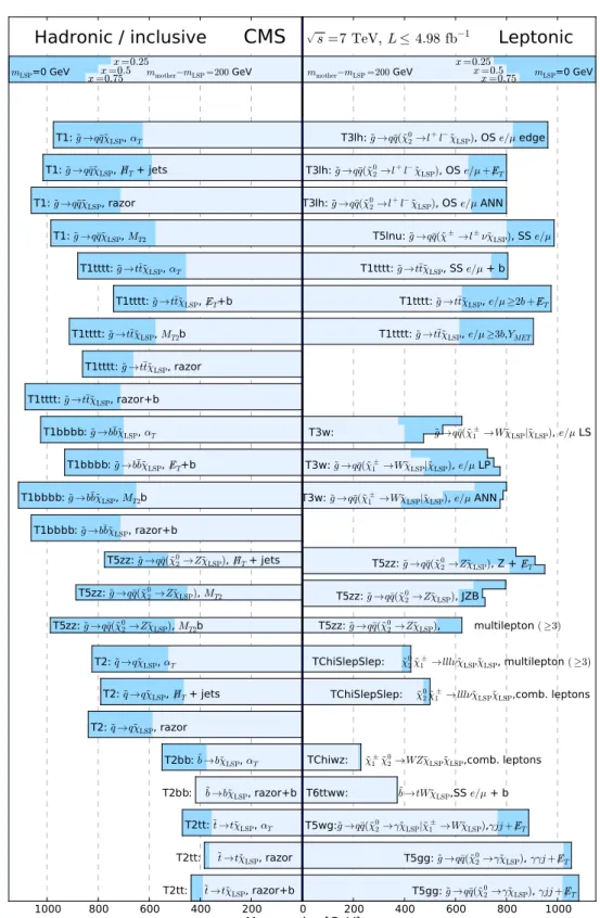
Figure 2 illustrates the results of the hadronic and inclusive analyses (left) and the leptonic analyses (right). Comparisons are made for two reference points of the mother and LSP masses:

[%] ε × A 0 5 10 15 20 25 30 35

gluino mass [GeV]

400 600 800 1000 L S P m a s s [ G e V ] 200 400 600 800 1000 1200 0 1 5 10 17 22 26 29 30 0 2 6 13 19 24 27 30 32 1 3 8 15 20 25 28 30 1 3 9 16 22 25 29 32 1 4 10 17 23 27 30 1 5 11 18 24 28 30 1 5 11 18 25 28 1 5 12 19 24 28 1 5 13 19 25 1 5 13 20 26 2 6 13 21 1 6 14 21 2 6 13 1 6 14 1 6 2 6 2 1 CMS ) g ~ ) + 0.5 m( LSP χ ∼ ) = 0.5 m( 2 0 χ ∼ m( -1 = 7 TeV, L = 4.98 fb s OS shape ) g ~ m( > ) > q ~ ); m( LSP χ ∼ -l + l → 2 0 χ∼ ( q q → g ~ g ~ → pp ) _s [fb] (CL σ 9 5 % C L u p p e r li m it o n 1 10 2 10 3 10 4 10

gluino mass [GeV]

400 600 800 1000 L S P m a s s [ G e V ] 200 400 600 800 1000 1200 1085 775 178 93 55 40 39 44 48 1752 358 122 57 56 43 36 35 105 747 195 80 50 35 29 29 31 342 155 58 39 29 25 22 21 321 124 52 37 26 20 22 353 94 44 32 21 19 20 281 93 42 29 21 18 248 92 37 26 20 16 230 84 35 25 17 228 85 32 23 20 271 73 32 19 275 68 30 20 238 64 31 270 57 28 250 60 205 57 233 269 CMS ) g ~ ) + 0.5 m( LSP χ ∼ ) = 0.5 m( 2 0 χ ∼ m( -1 = 7 TeV, L = 4.98 fb s OS shape ) g ~ m( > ) > q ~ ); m( LSP χ∼ -l + l → 2 0 χ ∼ ( q q → g ~ g ~ → pp (expected) NLO-NLL σ exp.) σ 1 ± (expected NLO-NLL σ (observed) NLO-NLL σ theor.) σ 1 ± (observed NLO-NLL σ [%] ε × A 0 5 10 15 20 25 30 35

gluino mass [GeV]

400 600 800 1000 L S P m a s s [ G e V ] 200 400 600 800 1000 1200 4 11 20 26 29 28 24 23 20 5 14 22 29 30 28 25 23 21 6 16 24 29 32 29 25 22 7 17 25 30 32 29 25 22 8 18 27 32 34 29 25 9 20 28 32 34 31 26 9 19 28 32 34 31 10 21 30 33 34 30 10 21 28 32 34 10 21 30 33 35 10 21 29 34 10 23 31 34 10 23 30 10 22 31 10 22 10 23 10 10 CMS ) g ~ ) + 0.5 m( LSP χ ∼ ) = 0.5 m( 2 0 χ ∼ m( -1 = 7 TeV, L = 4.98 fb s edge µ OS e/ ) g ~ m( > ) > q ~ ); m( LSP χ ∼ -l + l → 2 0 χ∼ ( q q → g ~ g ~ → pp ) _s [fb] (CL σ 9 5 % C L u p p e r li m it o n 1 10 2 10 3 10

gluino mass [GeV]

400 600 800 1000 L S P m a s s [ G e V ] 200 400 600 800 1000 1200 96 17 8 18 15 16 18 19 21 70 14 8 16 14 15 17 19 21 60 12 7 16 14 15 17 20 51 11 7 15 13 15 17 20 48 10 6 15 13 15 17 44 10 6 15 13 14 16 44 10 6 15 13 14 39 9 6 14 13 15 40 9 6 14 13 40 9 6 14 12 40 9 6 14 40 8 5 14 38 8 6 40 8 5 39 8 37 8 39 39 CMS ) g ~ ) + 0.5 m( LSP χ ∼ ) = 0.5 m( 2 0 χ ∼ m( -1 = 7 TeV, L = 4.98 fb s edge µ OS e/ ) g ~ m( > ) > q ~ ); m( LSP χ∼ -l + l → 2 0 χ ∼ ( q q → g ~ g ~ → pp (expected) NLO-NLL σ exp.) σ 1 ± (expected NLO-NLL σ (observed) NLO-NLL σ theor.) σ 1 ± (observed NLO-NLL σ

Figure 1: OS dileptons [21]: Product of the experimental efficiency and acceptance (left) and the upper limit on the product of the cross section and branching fraction (right) for the T3lh model from the E/ and HT T selection (top) and from edge reconstruction (bottom). Results are

shown as a function of gluino and LSP mass, with the intermediate neutralino mass set using x =0.5.

one with a massless LSP (M0, dark blue in Figure 2), one with a fixed mass splitting between the mother particle and the LSP of 200 GeV (∆M200, light blue in Figure 2). The results shown in Figure 2 are summarized below.

All-Hadronic This class of analyses sets limits on those models, such as T1, T2, and T5zz, that

produce several jets, but few leptons. The αT and 6HT+jets analyses yield similar limits

in the T1 and T2 models despite the differences in their event selections. In the case of the T5zz model, the MT2analysis is more sensitive to the model’s mass splitting than the

6HT+jets analysis: for M0, the MT2 analysis sets the stronger limit, while for∆M200 the

6

HT+jets analysis is more sensitive. This is expected, since the MT2 analysis uses a higher

cut on HTthan theH6 T+jets analysis. In general, the limits for the T5zz model are reduced

with respect to the T1 and T2 models, because of the reduced amount of E/ in cascadeT

decays.

1000 800 600 400 200 0 200 400 600 800 1000

Mass scales [GeV]

Hadronic / inclusive

Leptonic

mLSP=0 GeV _x=0x=0_.75.5 mmother−mLSP=200 GeV

x=0.25 mmother−mLSP=200 GeV x_x=0₌₀.5_.75 x=0.25 mLSP=0 GeV T2tt: ˜t→t˜χLSP, razor+b T5gg: ˜g→qq¯(˜χ02 →γ˜χLSP), γjj+6ET T2tt: ˜_t→t˜χLSP, razor T5gg: ˜g→qq¯(˜χ02 →γ˜χLSP), γγj+6ET T2tt: ˜_t→t˜χLSP, αT T5wg:˜g→q¯q(˜χ0 2 →γ˜χLSP|χ˜1 →± W˜χLSP),γjj+6ET T2bb: ˜_b→b˜χLSP, razor+b T6ttww: ˜b→tW˜χLSP,SS e/µ + b

T2bb: _b˜_→b˜χLSP, αT TChiwz: χ˜1±˜χ02 →WZ˜χLSP˜χLSP,comb. leptons

T2: ˜q→q˜χLSP, razor

T2: ˜q→q˜χLSP, 6HT + jets TChiSlepSlep: χ˜02χ˜1 →± lllν˜χLSP˜χLSP,comb. leptons

T2: ˜q→q˜χLSP, αT TChiSlepSlep: ˜χ20χ˜1 →± lllν˜χLSP˜χLSP, multilepton (≥3) T5zz: ˜g→q¯q(˜χ0 2 →Z˜χLSP), MT2b T5zz: ˜g→q¯q(˜χ0 2 →Z˜χLSP), multilepton (≥3) T5zz: ˜g→qq¯(˜χ0 2 →Z˜χLSP), MT2 T5zz: ˜g→q¯q(˜χ0 2 →Z˜χLSP), JZB T5zz: ˜g→q¯q(˜χ0 2 →Z˜χLSP), 6HT + jets T5zz: ˜g→q¯q(˜χ0 2 →Z˜χLSP), Z + 6ET T1bbbb: ˜g→b¯b˜χLSP, razor+b T1bbbb: ˜g→b¯b˜χLSP, MT2b T3w: ˜g→qq¯(˜χ± 1 →W˜χLSP|˜χLSP), e/µ ANN T1bbbb: ˜g→b¯b˜χLSP, 6ET+b T3w: ˜g→q¯q(˜χ1 →± Wχ˜LSP|˜χLSP), e/µ LP T1bbbb: ˜g→b¯bχ˜LSP, αT T3w: ˜g→q¯q(˜χ1 →± Wχ˜LSP|˜χLSP), e/µ LS T1tttt: ˜g→t¯t˜χLSP, razor+b T1tttt: ˜g→t¯_t˜χLSP, razor

T1tttt: ˜g→t¯t˜χLSP, MT2b T1tttt: ˜g→t¯t˜χLSP, e/µ≥3b,YMET

T1tttt: ˜g→t¯t˜χLSP, 6ET+b T1tttt: g˜→t¯t˜χLSP, e/µ≥2b+6ET

T1tttt: ˜g→t¯t˜χLSP, αT T1tttt: ˜g→t¯t˜χLSP, SS e/µ + b

T1: ˜g→q¯q˜χLSP, MT2 T5lnu: ˜g→qq¯(˜χ±→l±ν˜χLSP), SS e/µ

T1: ˜g→qq¯˜χLSP, razor T3lh: ˜g→q¯q(˜χ02 →l+l−˜χLSP), OS e/µ ANN

T1: ˜g→q¯q˜χLSP, 6HT + jets T3lh: ˜g→q¯q(˜χ02 →l+l−˜χLSP), OS e/µ+6ET

T1: ˜g→q¯qχ˜LSP, αT T3lh: ˜g→q¯q(˜χ02 →l+l−˜χLSP), OS e/µ edge

CMS

s

, L

.

Figure 2: Exclusion limits for the masses of the mother particles, for mLSP = 0 GeV (dark blue)

and mmother−mLSP=200 GeV (light blue), for each analysis, for the hadronic and razor results

(left) and the leptonic results (right). The limits are derived by comparing the allowed[σ× B]_UL

to the theory described in the text. For the T3, T5 and TChiSlepSlep models, the mass of the intermediate particle is defined by the relation mint = x mmother+ (1−x)mLSP. For the T3w

and T5zz models, the results are presented for x=0.25, 0.5, 0.75, while for the T3lh, T5lnu, and TChiSlepSlep models, x = 0.5. The lowest mass value for mmother depends on the particular

0 200 400 600 800 1000 1200

Mass scales [GeV]

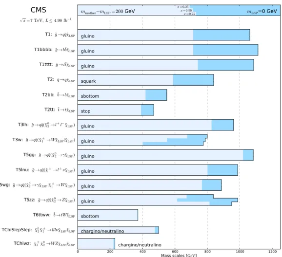
TChiwz: ˜χ± 1χ˜02→WZ˜χLSP˜χLSP TChiSlepSlep: ˜χ0 2χ˜1±→lllν˜χLSP˜χLSP T6ttww: ˜b→tW˜χLSP T5zz: ˜g→q¯q(˜χ0 2→Z˜χLSP) T5wg: ˜g→q¯q(˜χ0 2→γχ˜LSP|˜χ1±→Wχ˜LSP) T5lnu: ˜g→q¯q(˜χ±_→l±_ν˜χ LSP) T5gg: ˜g→q¯q(˜χ0 2→γχ˜LSP) T3w: ˜g→q¯q(˜χ± 1 →W˜χLSP|˜χLSP) T3lh: ˜g→q¯q(˜χ0 2→l+l−˜χLSP) T2tt: ˜t→t˜χLSP T2bb: ˜b→b˜χLSP T2: ˜q→q˜χLSP T1tttt: ˜g→t¯t˜χLSP T1bbbb: ˜g→b¯bχ˜LSP T1: ˜g→q¯q˜χLSP chargino/neutralino chargino/neutralino sbottom gluino gluino gluino gluino gluino gluino stop sbottom squark gluino gluino gluino mLSP=0 GeV mmother−mLSP=200 GeV x =0.50x =0.75 x =0.25

CMS

Figure 3: Best exclusion limits for the masses of the mother particles, for mLSP = 0 GeV (dark

blue) and m_mother−mLSP = 200 GeV (light blue), for each simplified model, for all analyses

considered. For the T3, T5 and TChiSlepSlep models, the mass of the intermediate particle is defined by the relation mint = x mmother+ (1−x)mLSP. For the T3w and T5zz models, the

results are presented for x = 0.25, 0.5, 0.75, while for the T3lh, T5lnu, and TChiSlepSlep mod-els, x = 0.5. The lowest mass value for mmother depends on the particular analysis and the

simplified model.

models, visible in Figure 2 (left). The three analyses set comparable limits for ∆M200, but the MT2b and αT analyses set the stronger limits for M0. For the T1tttt model, the

MT2b analysis is most sensitive.

The MT2b analysis is also compared with the MT2analysis with no b-tagging requirement.

The limit for the MT2b analysis on the T1bbbb model is stronger than for the MT2analysis

on the T1 model, since many of the backgrounds are removed by requiring a b-tagged jet, allowing for a lower threshold on the MT2variable. Also, the limit on the T5zz model

from the MT2b analysis is stronger than for the MT2 analysis, even though the b-tagged

jets from the T5zz model arise mainly through the decay Z→bb.

Single Lepton + Jets This class of analyses is sensitive to simplified models that produce W bosons

or direct decays to leptons. The e/µ LS, LP, and ANN analyses set limits on the T3w model for an intermediate (chargino) mass corresponding to x= 1₄,1₂, and3₄.

The LS and LP analyses are sensitive to the kinematic properties of the W boson produced in the chargino decay. For a large mass splitting between the mother and LSP (M0), the

LP and ANN limits are less sensitive to x than the LS limit. For a fixed mass splitting (∆M200), however, the ANN limit is more sensitive. The limits for M0 are stronger for all three analyses, with LP and ANN setting the best limits.

The e/µ≥2b+E/ and e/µT ≥3b, YMETanalyses set limits on the T1tttt model.

Opposite-Sign Dileptons The Z+E/ and JZB analyses both set limits on the T5zz model rely-T

ing on the leptonic decays of one of the Z bosons. The Z+E/ analysis sets the strongerT

limit for x = 3₄ and M0, for which more E/ is produced on average. The JZB analysisT

has the opposite behavior, since the separation between signal and background in the JZB variable is maximized in the signal when the E/ and Z-pT T vectors point in the same

direction. Therefore, the best limit is set for x= 1₄.

Limits are also set on the T3lh model, with the non-resonant decay of the intermediate neutralino to leptons, by the E/ , the edge-based, and the neural-network-based analyses.T

The edge-based analysis sets significantly stronger limits.

Same-Sign Dileptons The T5lnu model produces equal numbers of OS and SS dileptons.

Lim-its are set on the T5lnu model by the SS dilepton analysis. No comparisons are made for the OS dilepton analyses as these are expected to be much less sensitive due to their larger backgrounds.

The SS dilepton analysis with a b-tagged jet is used to set limits on the T1tttt and the T6ttww models. The analysis is not strongly sensitive to mass splittings, and a similar limit is set for the case of M0 or∆M200.

Multileptons Limits are set on the TChiSlepSlep model, which produces leptons through

slep-ton decays but not through gauge-boson decays. A limit is set on the chargino mass (which equals the heavy neutralino mass) near 500 GeV, which is not strongly dependent on the mass splitting. The limits on the model TChiwz are significantly reduced because of the corresponding reduction from the branching fraction of the gauge bosons into lep-tons. A limit on the T5zz model is also set. For the∆M200 case the limit is competitive with the limits set by the hadronic analyses, despite the low Z→ `+<sub>`</sub>−_{branching fraction.}

Photons Limits are set on the T5gg and T5wg models, which produce two isolated photons

and E/ or one isolated photon and ET / , respectively. The one- and two-photon analysesT

set comparable limits on the T5gg model. In addition, the one-photon analysis sets a competitive limit on the T5wg model.

Inclusive The razor and razor+b analyses set limits on the T1, T2, T1bbbb, T1tttt, T2bb, and

T2tt models. The limits on each of these models are comparable with the best limits set by individual, exclusive analyses.

Figure 3 illustrates the best hadronic or leptonic result for each simplified model. Excluding the photon signatures, the best limits for the M0 scenario exclude gluino masses below 1 TeV and squark masses below 800 GeV. For the ∆M200 scenario, the limit is reduced to near 800 GeV and 600 GeV, respectively. The limits on the gluino mass from the photon signatures are near 1.1 TeV, regardless of the mass splitting.

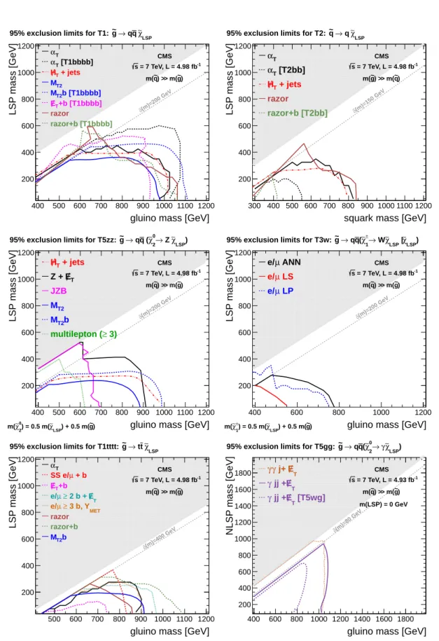
Figure 4 illustrates the exclusion contours in the two-dimensional plane of the mother versus LSP mass for the T1 (T1bbbb), T2 (T2bb), T5zz, T3w, T1tttt and T5gg (T5wg) models. The results shown in Figures 2 and 3 are a subset of these results. Regions where the analyses, due to the uncertainty in the acceptance calculation, do not produce a limit are denoted by dashed lines. Figure 4 (upper-left) shows the exclusion contours of the T1 and T1bbbb models using

the hadronic and b-tagged hadronic analyses. This tests the dependence on the assumption of whether the gluino decays to light or heavy flavors. Solid (dashed) lines are used for the T1 (T1bbbb) model. The αT analysis covers a larger area in the gluino-LSP mass plane for the

T1bbbb model than the hadronic decays do for the T1 model. However, this comparison is only valid if the gluino indeed decays only to bottom quarks. The fully hadronic 6HT+jets and αT

analyses cover a similar region, while the MT2analysis covers comparatively less. The inclusive

analysis is particularly sensitive when the difference in mass between the mother and LSP is small, a situation known as a “compressed spectrum.”

Figure 4 (upper-right) compares the exclusion contours of the T2 and T2bb models. The αT and

6HT+jets analyses set similar limits on the T2 model. The αTanalysis sets weaker limits on the

T2bb model, but the reference cross section is a factor of eight smaller than for the T2 model. The inclusive analysis sets the overall strongest limits, particularly in the low mass splitting region.

Figure 4 (middle-left) compares the exclusion contours of the T5zz model. The T5zz model comparison demonstrates the complementarity of leptonic, hadronic, and b-tagged hadronic analyses. In particular, the leptonic analyses are more limiting for smaller mass splittings, while the hadronic analyses are more limiting for larger gluino masses.

Figure 4 (middle-right) compares the exclusion contours of the T3w model. The e/µ ANN and e/µ LP analyses provide comparable results. The e/µ LS spectrum analysis excludes a smaller region.

Figure 4 (bottom-left) compares the exclusion contours of the T1tttt model. The inclusive anal-ysis with b-tagged jets sets the strongest limit on the gluino mass. The SS+b analanal-ysis, however, sets limits that are almost independent of mass splitting.

Figure 4 (bottom-right) compares the exclusion contours of the T5gg and T5wg models. The limits on the T5gg and T5wg models demonstrate the insensitivity of these photon analyses to the NLSP mass. Also, the requirement on the number of photons (one or two) has little effect on the limit on the T5gg model. The limit on the T5wg model, which has only one signal photon per event, excludes a smaller region than the limit on the T5gg model.

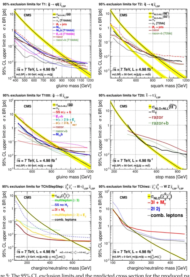
Figure 5 shows values of[σ× B]_ULfor the T1 (T1bbbb), T2 (T2bb), T1tttt, T2tt, TChiSlepSlep,

and TChiwz models as functions of the produced particle masses at fixed values of the LSP mass. In the top and middle figures, the LSP mass is fixed at 50 GeV, while in the lower figures the LSP is fixed to be massless. Figure 5 also illustrates the method for translating an upper limit on[σ× B]_ULto a lower limit on the mass of a hypothetical particle. For example, Figure 5

(top-left) displays[σ× B]_UL for the various analyses that are sensitive to the T1 and T1bbbb

models. These limits can be compared to σNLO+NLL for gluino pair production as a function of gluino mass. The intersection of σNLO+NLLwith[σ× B]_UL determines a lower limit on the

gluino mass. The analyses set a lower limit of approximately 1 TeV on the gluino mass for a LSP mass of 50 GeV, corresponding to an upper limit on the cross section of approximately 10 fb. This limit assumes B = 1 for the decay of each gluino to a light-flavor quark-antiquark pair and the LSP. The (yellow) band on the σNLO+NLLcurve represents an estimate of the theoretical uncertainties on the cross section calculation. This figure also demonstrates the decrease in [σ× B]_ULand the increase on the upper limit on the gluino mass for those analyses sensitive to

the T1bbbb model.

Similar comparisons can be performed for the different simplified models. For example, Fig-ure 5 (top-right) displays [σ× B]_UL for the various analyses that are sensitive to the T2 and

a LSP mass of 50 GeV, corresponding to an upper limit on the cross section of approximately 10 fb. This limit assumes there are four squarks with the same mass and that B = 1 for the decay of each squark to a light-flavor quark and the LSP. If only bottom squark-antisquark pro-duction is considered, and each bottom squark decays to a bottom quark and the LSP, a lower limit of approximately 550 GeV is set on the bottom squark mass for a LSP mass of 50 GeV, cor-responding to an upper limit on the cross section of approximately 20 fb. Figure 5 (bottom-left) displays the limits on the model TChiSlepSlep. A chargino mass of approximately 550 GeV is excluded, corresponding to an upper limit on the cross section of approximately 2 fb. This limit assumes thatB =1 for the decay of the chargino and neutralino to sleptons that further decay to leptons and LSPs. For the model TChiwz, the limit decreases to 220 GeV, corresponding to an upper limit on the cross section of approximately 30 fb. This limit assumes thatB =1 for the decay of the chargino to a W boson and the LSP and the decay of the neutralino to a Z boson and the LSP.

Many of the interpretations presented in Figure 4 exclude a gluino mass of less than approx-imately 1 TeV for a range of LSP masses ranging from 200 to 400 GeV. However, the exclu-sion of a particle mass in a simplified model using SUSY cross sections involves assumptions. For example, the σNLO+NLLcalculation for gluino pair production depends upon the choice of squark masses. If the light-flavor squarks in a specific model, rather than being decoupled, have masses of a few TeV, the predicted gluino cross sections drop significantly due to destruc-tive interference between different amplitudes. The limits on models with cascade decays, T3w, T5lnu, and T5zz, assume a branching fraction of unity for a gluino decay to a chargino or neutralino. However, a realistic MSSM model would contain a degenerate chargino-neutralino pair, reducing the branching fraction to 1₂ or 1₄. Furthermore it should be noted that the lower limits on the sparticle masses have been derived for cross sections based on the spin assumed in the CMSSM. Also, the model T2 assumes degenerate copies of left– and right–handed light-flavor squarks, while a realistic model may have a significant mass hierarchy between different squark flavors or eigenstates. As mentioned earlier, the model T2tt has no spin correlation between the neutralino and the top quark decay products, while such a correlation will arise in the MSSM depending on the mixture of interaction quantum states in the mass quantum states of the top squark and the neutralino. The information contained in this paper and in the supplementary references can be used to set limits if any of these assumptions, or others, are removed or weakened. It must also be noted that the exclusion limits discussed here only serve to broadly summarize simplified model results; the full information on the exclusion power of an analysis in the context of simplified models is contained in the exclusion limits on the production cross section, as shown in Figure 1. This information is contained in the analysis references. A final caveat can be made regarding the setting of limits in simplified models. Since only one signal process is considered, potential backgrounds are ignored from other signal processes that may arise in a complete model.

6

Summary

The simplified model framework is a recently-developed method for interpreting the results of searches for new physics. This paper contains a compilation of simplified model interpre-tations of CMS supersymmetry analyses based on 2011 data. For each simplified model and analysis, an upper limit on the product of the cross section and branching fraction is derived as a function of hypothetical particle masses. Additionally, lower limits on particle masses are determined by comparing the 95% CL upper limit on the product of the cross section and branching fraction to the predicted cross section in Supersymmetry for the pair of primary par-ticles. These lower limits depend upon theoretical assumptions that are described earlier in this

gluino mass [GeV] 400 500 600 700 800 900 1000 1100 1200 L S P m a s s [ G e V ] 200 400 600 800 1000 1200 (m)=200 GeV δ T α [T1bbbb] T α + jets T H T2 M b [T1bbbb] T2 M +b [T1bbbb] T E razor razor+b [T1bbbb] CMS LSP χ∼ q q → g ~ 95% exclusion limits for T1:

-1 = 7 TeV, L = 4.98 fb s ) g ~ m( > ) > q ~ m(

squark mass [GeV]

300 400 500 600 700 800 900 1000 1100 1200 L S P m a s s [ G e V ] 200 400 600 800 1000 1200 (m)=150 GeV δ T α [T2bb] T α + jets T H razor razor+b [T2bb] CMS LSP χ∼ q → q ~ 95% exclusion limits for T2:

-1 = 7 TeV, L = 4.98 fb s ) q ~ m( > ) > g ~ m(

gluino mass [GeV]

400 500 600 700 800 900 1000 1100 1200 L S P m a s s [ G e V ] 200 400 600 800 1000 1200 (m)=200 GeV δ + jets T H T E Z + JZB T2 M b T2 M 3) ≥ multilepton ( CMS ) LSP χ∼ Z → 2 0 χ∼ ( q q → g ~ 95% exclusion limits for T5zz:

-1 = 7 TeV, L = 4.98 fb s ) g ~ m( > ) > q ~ m( ) g ~ ) + 0.5 m( LSP χ∼ ) = 0.5 m( 2 0 χ∼

m( gluino mass [GeV]

400 600 800 1000 1200 L S P m a s s [ G e V ] 200 400 600 800 1000 1200 (m)=200 GeV δ ANN µ e/ LS µ e/ LP µ e/ CMS ) LSP χ∼ | LSP χ∼ W → 1 ± χ∼ ( q q → g ~ 95% exclusion limits for T3w:

-1 = 7 TeV, L = 4.98 fb s ) g ~ m( > ) > q ~ m( ) g ~ ) + 0.5 m( LSP χ∼ ) = 0.5 m( 1 ± χ∼ m(

gluino mass [GeV]

500 600 700 800 900 1000 1100 1200 L S P m a s s [ G e V ] 200 400 600 800 1000 1200 (m)=400 GeV δ T α + b µ SS e/ +b T E T E 2 b + ≥ µ e/ MET 3 b, Y ≥ µ e/ razor razor+b b T2 M CMS LSP χ∼ t t → g ~ 95% exclusion limits for T1tttt:

-1 = 7 TeV, L = 4.98 fb s ) g ~ m( > ) > q ~ m(

gluino mass [GeV]

400 600 800 1000 1200 1400 1600 1800 N L S P m a s s [ G e V ] 200 400 600 800 1000 1200 1400 1600 1800 (m)=80 GeV δ T E j+ γ γ T E jj + γ [T5wg] T E jj + γ CMS m(LSP) = 0 GeV ) LSP χ∼ γ → 2 0 χ∼ ( q q → g ~ 95% exclusion limits for T5gg:

-1 = 7 TeV, L = 4.93 fb s ) g ~ m( > ) > q ~ m(

Figure 4: The 95% CL exclusion limits on the produced particle and LSP masses in the models T1(T1bbbb), T2(T2bb), T5zz, T3w, T1tttt, and T5gg(T5wg). The grey area represents the region where the decay mode is forbidden.

gluino mass [GeV] 400 500 600 700 800 900 1000 1100 1200 x BR [pb] σ 9 5 % C L u p p e r lim it o n -3 10 -2 10 -1 10 1 10 LSP χ ∼ q q → g ~ 95% exclusion limits for T1:

-1 = 7 TeV, L = 4.98 fb s ) g ~ m( > ) > q ~ m(LSP) = 50 GeV, m( CMS σNLO+NLL(g~g~) T α [T1bbbb] T α + jets T H T2 M b [T1bbbb] T2 M +b [T1bbbb] T E razor razor+b [T1bbbb]

squark mass [GeV]

400 600 800 1000 1200 x BR [pb] σ 9 5 % C L u p p e r lim it o n -3 10 -2 10 -1 10 1 10 LSP χ ∼ q → q ~ 95% exclusion limits for T2:

-1 = 7 TeV, L = 4.98 fb s ) b ~ m( > ) > q ~ , g ~ m(LSP) = 50 GeV, m( CMS σNLO+NLL(q~q~*) ) * b ~ b ~ ( NLO+NLL σ T α [T2bb] T α + jets T H razor razor+b [T2bb]

gluino mass [GeV]

600 800 1000 1200 x BR [pb] σ 9 5 % C L u p p e r lim it o n -3 10 -2 10 -1 10 1 10 2 10 LSP χ ∼ t t → g ~ 95% exclusion limits for T1tttt:

-1 = 7 TeV, L = 4.98 fb s ) g ~ m( > ) > q ~ m(LSP) = 50 GeV, m( CMS σNLO+NLL(g~g~) T α + b µ SS e/ +b T E T E 2 b + ≥ µ e/ MET 3 b, Y ≥ µ e/ razor razor+b b T2 M

stop mass [GeV]

200 400 600 800 x BR [pb] σ 9 5 % C L u p p e r lim it o n -3 10 -2 10 -1 10 1 10 LSP χ ∼ t → t ~ 95% exclusion limits for T2tt:

-1 = 7 TeV, L = 4.98 fb s ) t ~ m( > ) > q ~ , g ~ m(LSP) = 50 GeV, m( CMS σ_NLO+NLL(~t~t*₎ T α razor razor+b

chargino/neutralino mass [GeV]

200 400 600 x BR [pb] σ 9 5 % C L u p p e r lim it o n -4 10 -3 10 -2 10 -1 10 1 10 LSP χ ∼ LSP χ ∼ ν lll → 1 ± χ ∼ 2 0 χ ∼ 95% exclusion limits for TChiSlepSlep:

-1 = 7 TeV, L = 4.98 fb s ) 1 ± χ ∼ ),m( 2 0 χ ∼ m( > ) > q ~ ),m( g ~ m(LSP) = 0 GeV, m( CMS ) LSP χ ∼ ) + 0.5 m( 2 0 χ ∼ | 1 ± χ ∼ ) = 0.5 m( l ~ m( ) 1 ± χ ∼ 2 0 χ ∼ ( NLO σ 3) ≥ multilepton ( T SS no H T 3l + M T E 3) + ≥ multilepton ( comb. leptons

chargino/neutralino mass [GeV]

100 200 300 400 x BR [pb] σ 9 5 % C L u p p e r lim it o n -2 10 -1 10 1 10 2 10 LSP χ ∼ LSP χ ∼ W Z → 2 0 χ ∼ 1 ± χ ∼ 95% exclusion limits for TChiwz:

-1 = 7 TeV, L = 4.98 fb s ) 1 ± χ ∼ ),m( 2 0 χ ∼ m( > ) > q ~ ),m( g ~ m(LSP) = 0 GeV, m( CMS ) 1 ± χ ∼ 2 0 χ ∼ ( NLO σ T 3l + M 2l 2j comb. leptons

Figure 5: The 95% CL exclusion limits and the predicted cross section for the produced particle masses with a fixed LSP mass in the models T1(T1bbbb), T2(T2bb), T1tttt, T2tt, TChiSlepSlep and TChiwz.

paper. They should not be regarded as general exclusions on Supersymmetric particle masses. The most stringent results for a few simplified models are summarized here. If the primary particles are gluinos that each decay to quark-antiquark pair and a neutralino, a gluino of mass of approximately 1 TeV is excluded for a neutralino of mass 50 GeV. These masses correspond to an upper limit on the gluino pair production cross section of approximately 10 fb. The ex-cluded mass increases if each gluino decays to a bottom quark-antiquark pair and a neutralino, while the excluded mass decreases if each gluino decays to a top quark-antiquark pair and a neutralino. The excluded mass also decreases if the gluino undergoes a cascade of decays. If the primary particles are four squark-antisquark pairs, and each squark decays to a light-flavor quark and a neutralino, a squark mass of approximately 800 GeV is excluded for a neutralino of mass 50 GeV, corresponding to an upper limit on the squark-antisquark production cross section of approximately 10 fb. The excluded mass for a single bottom-antibottom squark pair is 550 GeV. The comparable exclusion in mass for a single top-antitop squark pair is approxi-mately 150 GeV lower. In the case of the electroweak production of a chargino-neutralino pair, the upper limit on the cross section is approximately one order of magnitude higher than the corresponding limit for gluino pair production at the same mass.

The predictions for experimental acceptance and exclusion limits on cross sections presented here for a range of simplified models and mass parameters can be used to constrain other theoretical models and compare different analyses.

Acknowledgments

We congratulate our colleagues in the CERN accelerator departments for the excellent perfor-mance of the LHC and thank the technical and administrative staffs at CERN and at other CMS institutes for their contributions to the success of the CMS effort. In addition, we gratefully acknowledge the computing centres and personnel of the Worldwide LHC Computing Grid for delivering so effectively the computing infrastructure essential to our analyses. Finally, we acknowledge the enduring support for the construction and operation of the LHC and the CMS detector provided by the following funding agencies: the Austrian Federal Ministry of Science and Research; the Belgian Fonds de la Recherche Scientifique, and Fonds voor Wetenschap-pelijk Onderzoek; the Brazilian Funding Agencies (CNPq, CAPES, FAPERJ, and FAPESP); the Bulgarian Ministry of Education, Youth and Science; CERN; the Chinese Academy of Sciences, Ministry of Science and Technology, and National Natural Science Foundation of China; the Colombian Funding Agency (COLCIENCIAS); the Croatian Ministry of Science, Education and Sport; the Research Promotion Foundation, Cyprus; the Ministry of Education and Re-search, Recurrent financing contract SF0690030s09 and European Regional Development Fund, Estonia; the Academy of Finland, Finnish Ministry of Education and Culture, and Helsinki Institute of Physics; the Institut National de Physique Nucl´eaire et de Physique des Partic-ules / CNRS, and Commissariat `a l’ ´Energie Atomique et aux ´Energies Alternatives / CEA, France; the Bundesministerium f ¨ur Bildung und Forschung, Deutsche Forschungsgemeinschaft, and Helmholtz-Gemeinschaft Deutscher Forschungszentren, Germany; the General Secretariat for Research and Technology, Greece; the National Scientific Research Foundation, and Na-tional Office for Research and Technology, Hungary; the Department of Atomic Energy and the Department of Science and Technology, India; the Institute for Studies in Theoretical Physics and Mathematics, Iran; the Science Foundation, Ireland; the Istituto Nazionale di Fisica Nu-cleare, Italy; the Korean Ministry of Education, Science and Technology and the World Class University program of NRF, Republic of Korea; the Lithuanian Academy of Sciences; the Mex-ican Funding Agencies (CINVESTAV, CONACYT, SEP, and UASLP-FAI); the Ministry of

Sci-ence and Innovation, New Zealand; the Pakistan Atomic Energy Commission; the Ministry of Science and Higher Education and the National Science Centre, Poland; the Fundac¸˜ao para a Ciˆencia e a Tecnologia, Portugal; JINR (Armenia, Belarus, Georgia, Ukraine, Uzbekistan); the Ministry of Education and Science of the Russian Federation, the Federal Agency of Atomic En-ergy of the Russian Federation, Russian Academy of Sciences, and the Russian Foundation for Basic Research; the Ministry of Science and Technological Development of Serbia; the Secretar´ıa de Estado de Investigaci ´on, Desarrollo e Innovaci ´on and Programa Consolider-Ingenio 2010, Spain; the Swiss Funding Agencies (ETH Board, ETH Zurich, PSI, SNF, UniZH, Canton Zurich, and SER); the National Science Council, Taipei; the Thailand Center of Excellence in Physics, the Institute for the Promotion of Teaching Science and Technology of Thailand and the Na-tional Science and Technology Development Agency of Thailand; the Scientific and Technical Research Council of Turkey, and Turkish Atomic Energy Authority; the Science and Technology Facilities Council, UK; the US Department of Energy, and the US National Science Foundation. Individuals have received support from the Marie-Curie programme and the European Re-search Council (European Union); the Leventis Foundation; the A. P. Sloan Foundation; the Alexander von Humboldt Foundation; the Belgian Federal Science Policy Office; the Fonds pour la Formation `a la Recherche dans l’Industrie et dans l’Agriculture (FRIA-Belgium); the Agentschap voor Innovatie door Wetenschap en Technologie (IWT-Belgium); the Ministry of Education, Youth and Sports (MEYS) of Czech Republic; the Council of Science and Industrial Research, India; the Compagnia di San Paolo (Torino); and the HOMING PLUS programme of Foundation for Polish Science, cofinanced from European Union, Regional Development Fund.

References

[1] J. Wess and B. Zumino, “Supergauge transformations in four dimensions”, Nucl. Phys. B

70(1974) 39, doi:10.1016/0550-3213(74)90355-1.

[2] A. H. Chamseddine, R. Arnowitt, and P. Nath, “Locally Supersymmetric Grand Unification”, Phys. Rev. Lett. 49 (1982) 970, doi:10.1103/PhysRevLett.49.970. [3] R. Arnowitt and P. Nath, “Supersymmetric mass spectrum in SU(5) supergravity grand

unification”, Phys. Rev. Lett. 69 (1992) 725, doi:10.1103/PhysRevLett.69.725. [4] G. L. Kane, C. F. Kolda, L. Roszkowski, and J. D. Wells, “Study of constrained minimal

supersymmetry”, Phys. Rev. D 49 (1994) 6173, doi:10.1103/PhysRevD.49.6173, arXiv:hep-ph/9312272.

[5] N. Arkani-Hamed et al., “MARMOSET: The Path from LHC Data to the New Standard Model via On-Shell Effective Theories”, (2007). arXiv:hep-ph/0703088.

[6] J. Alwall, P. C. Schuster, and N. Toro, “Simplified models for a first characterization of new physics at the LHC”, Phys. Rev. D 79 (2009) 075020,

doi:10.1103/PhysRevD.79.075020, arXiv:0810.3921.

[7] J. Alwall, M.-P. Le, M. Lisanti, and J. G. Wacker, “Model-Independent Jets plus Missing Energy Searches”, Phys. Rev. D 79 (2009) 015005,

doi:10.1103/PhysRevD.79.015005, arXiv:0809.3264.

[8] D. S. M. Alves, E. Izaguirre, and J. G. Wacker, “Where the sidewalk ends: jets and missing energy search strategies for the 7 TeV LHC”, JHEP 10 (2011) 012,

[9] LHC New Physics Working Group Collaboration, “Simplified models for LHC new physics searches”, J. Phys. G 39 (2012) 105005,

doi:10.1088/0954-3899/39/10/105005, arXiv:1105.2838.

[10] M. Papucci, J. T. Ruderman, and A. Weiler, “Natural SUSY endures”, JHEP 09 (2012) 035,

doi:10.1007/JHEP09(2012)035, arXiv:1110.6926.

[11] R. Mahbubani et al., “Light non-degenerate squarks at the LHC”, Phys. Rev. Lett. 110 (2013) 151804, doi:10.1103/PhysRevLett.110.151804, arXiv:1212.3328. [12] CMS Collaboration, “Search for supersymmetry in final states with missing transverse

energy and 0, 1, 2, or at least 3 b-quark jets in 7 TeV pp collisions using the variable αT”,

JHEP 1301 (2013) 077, doi:10.1007/JHEP01(2013)077, arXiv:1210.8115. [13] CMS Collaboration, “Search for new physics in the multijet and missing transverse

momentum final state in proton-proton collisions at√s = 7 TeV”, Phys. Rev. Lett. 109 (2012) 171803, doi:10.1103/PhysRevLett.109.171803, arXiv:1207.1898. [14] CMS Collaboration, “Search for supersymmetry in hadronic final states using MT2in pp

collisions at√s = 7 TeV”, JHEP 10 (2012) 018, doi:10.1007/JHEP10(2012)018, arXiv:1207.1798.

[15] CMS Collaboration, “Search for supersymmetry in events with b-quark jets and missing transverse energy in pp collisions at 7 TeV”, Phys. Rev. D 86 (2012) 072010,

doi:10.1103/PhysRevD.86.072010, arXiv:1208.4859.

[16] CMS Collaboration, “Inclusive search for supersymmetry using the razor variables in pp collisions at√s = 7 TeV”, (2012). arXiv:1212.6961. Submitted to Phys. Rev. Lett. [17] CMS Collaboration, “Search for supersymmetry in pp collisions at√s=7 TeV in events

with a single lepton, jets, and missing transverse momentum”, Eur. Phys. J. C 73 (2013) 2404, doi:10.1140/epjc/s10052-013-2404-z, arXiv:1212.6428.

[18] CMS Collaboration, “Search for supersymmetry in final states with a single lepton, b-quark jets, and missing transverse energy in proton-proton collisions at√s = 7 TeV”, Phys. Rev. D 87 (2013) 052006, doi:10.1103/PhysRevD.87.052006,

arXiv:1211.3143.

[19] CMS Collaboration, “Search for new physics with same-sign isolated dilepton events with jets and missing transverse energy”, Phys. Rev. Lett. 109 (2012) 071803,

doi:10.1103/PhysRevLett.109.071803, arXiv:1205.6615.

[20] CMS Collaboration, “Search for new physics in events with same-sign dileptons and b-tagged jets in pp collisions at√s = 7 TeV”, JHEP 08 (2012) 110,

doi:10.1007/JHEP08(2012)110, arXiv:1205.3933.

[21] CMS Collaboration, “Search for new physics in events with opposite-sign leptons, jets, and missing transverse energy in pp collisions at√s = 7 TeV”, Phys. Lett. B 718 (2013) 815, doi:10.1016/j.physletb.2012.11.036, arXiv:1206.3949.

[22] CMS Collaboration, “Search for supersymmetry in events with opposite-sign dileptons and missing transverse energy using an artificial neural network”, Phys. Rev. D 87 (2013) 072001, doi:10.1103/PhysRevD.87.072001, arXiv:1301.0916.

[23] CMS Collaboration, “Search for anomalous production of multilepton events in pp collisions at√s =7 TeV”, JHEP 06 (2012) 169, doi:10.1007/JHEP06(2012)169, arXiv:1204.5341.

[24] CMS Collaboration, “Search for electroweak production of charginos and neutralinos using leptonic final states in pp collisions at√s = 7 TeV”, JHEP 11 (2012) 147,

doi:10.1007/JHEP11(2012)147, arXiv:1209.6620.

[25] CMS Collaboration, “Search for physics beyond the standard model in events with a Z boson, jets, and missing transverse energy in pp collisions at√s = 7 TeV”, Phys. Lett. B

716(2012) 260, doi:10.1016/j.physletb.2012.08.026, arXiv:1204.3774.

[26] CMS Collaboration, “Search for new physics in events with photons, jets, and missing transverse energy in pp collisions at√s = 7 TeV”, JHEP 03 (2013) 111,

doi:10.1007/JHEP03(2013)111, arXiv:1211.4784.

[27] CMS Collaboration, “Search for New Physics with Jets and Missing Transverse Momentum in pp collisions at√s = 7 TeV”, JHEP 08 (2011) 155,

doi:10.1007/JHEP08(2011)155, arXiv:1106.4503.

[28] ATLAS Collaboration, “Search for squarks and gluinos with the ATLAS detector in final states with jets and missing transverse momentum using 4.7 fb−1of√s = 7 TeV

proton-proton collision data”, Phys. Rev. D 87 (2013) 012008, doi:10.1103/PhysRevD.87.012008, arXiv:1208.0949.

[29] ATLAS Collaboration, “Search for top and bottom squarks from gluino pair production in final states with missing transverse energy and at least three b-jets with the ATLAS detector”, Eur. Phys. J. C 72 (2012) 2174, doi:10.1140/epjc/s10052-012-2174-z,

arXiv:1207.4686.

[30] ATLAS Collaboration, “Search for direct slepton and gaugino production in final states with two leptons and missing transverse momentum with the ATLAS detector in pp collisions at√s = 7 TeV”, Phys. Lett. B 718 (2013) 879,

doi:10.1016/j.physletb.2012.11.058, arXiv:1208.2884.

[31] ATLAS Collaboration, “Search for direct production of charginos and neutralinos in events with three leptons and missing transverse momentum in√s = 7 TeV pp collisions with the ATLAS detector”, Phys. Lett. B 718 (2013) 841,

doi:10.1016/j.physletb.2012.11.039, arXiv:1208.3144.

[32] ATLAS Collaboration, “Search for supersymmetry in pp collisions at√s = 7 TeV in final states with missing transverse momentum and b-jets with the ATLAS detector”, Phys. Rev. D 85 (2012) 112006, doi:10.1103/PhysRevD.85.112006, arXiv:1203.6193. [33] ATLAS Collaboration, “Hunt for new phenomena using large jet multiplicities and

missing transverse momentum with ATLAS in 4.7 fb−1of√s = 7 TeV proton-proton collisions”, JHEP 07 (2012) 167, doi:10.1007/JHEP07(2012)167,

arXiv:1206.1760.

[34] ATLAS Collaboration, “Further search for supersymmetry at√s=7 TeV in final states with jets, missing transverse momentum and isolated leptons with the ATLAS detector”, Phys. Rev. D 86 (2012) 092002, doi:10.1103/PhysRevD.86.092002,