Composição química do aerossol europeu

(1)

Universidade de Aveiro Departamento de Ambiente e Ordenamento 2008

ALEXANDRE FILIPE

FERNANDES

CASEIRO

COMPOSIC

¸ ˜

AO QU´IMICA DO AEROSSOL

(2)

(3)

Universidade de Aveiro Departamento de Ambiente e Ordenamento 2008

ALEXANDRE FILIPE

FERNANDES

CASEIRO

COMPOSIC

¸ ˜

AO QU´IMICA DO AEROSSOL

EUROPEU

Disserta¸cão apresentada à Universidade de Aveiro para cumprimento dos requesitos necessários à obten¸cão do grau de doutor em Ciências do Ambi-ente, realizada sob a orienta¸cão cient´ıfica do doutor Casimiro Adrião Pio, Professor do Departamento de Ambiente e Ordenamento da Universidade de Aveiro e do doutor Hans Puxbaum, Full Professor do Institut für Chemische Technologien und Analytik da Technische Universität Wien.

Apoio financeiro da FCT no ˆambito da bolsa de doutora-mento SFRH/BD/42145/2007

(4)

(5)

(6)

(7)

o j´uri / the jury

presidente / president Maria Helena Nazar´e

Reitora da Universidade de Aveiro

vogais / examiners committee Doutora Maria Teresa S´a Dias de Vasconcelos

Professora Catedr´atica do Departamento de Qu´ımica da Faculdade de Ciˆencias da Universidade do Porto

Doutor Casimiro Adri˜ao Pio

Professor Catedr´atico do Departamento de Ambiente e Ordenamento da Universi-dade de Aveiro (orientador)

Doutor Hans Puxbaum

Full Professor do Institute for Analytical Chemistry da University of Technology de Viena, ´Austria (co-orientador)

Doutora Bego˜na Art´ı˜nano Rodriguez de Torres

Senior Scientist do Environment Department do CIEMAT, Ministry of Science and Innovation, Madrid, Espanha

Doutor Valdemar Inocˆencio Esteves

Professor Auxiliar, Departamento de Qu´ımica da Universidade de Aveiro Doutora C´elia dos Anjos Alves

Equiparada a Investigadora Auxiliar, CESAM–Centro de Estudos do Ambiente e do Mar da Universidade de Aveiro

(8)

(9)

agradecimentos / acknowledgements

Agrade¸co aos meus orientadores por terem acreditado nas minhas ca-pacidades. Agrade¸co ao meu orientador, Pr. Dr. Casimiro Adrião Pio, a oportunidade de evoluir na minha aprendizagem que me foi concedida através deste doutoramento. Também agrade¸co ao meu co-orientador, Ao.Univ.Prof. Dipl.-Ing. Dr.techn. Hans Puxbaum, pela oportunidade que foi integrar o seu grupo de trabalho e pelo conhecimento que lá me foi permitido adquirir. Quero ainda agradecer aos meus coelgas da TU Wien, com o apoio de quem o trabalho laboratorial se tournou poss´ıvel, e muito especialmente à Ao.Univ.Prof. Dipl.-Ing. Dr.techn. Anneliese Kasper-Giebl, pelo acompanhamento e confian¸ca excepcionais. Também desejo agradecer o apoio dos colegas do DAO, muito especialmente na fase de reda¸cão deste trabalho.

I thank my supervisors for believing in my capabilities. I thank my supervisor, Pr. Dr. Casimiro Adri˜ao Pio, the opportunity to evolve in my learning process that was conceded to me by this Ph. D. I also thank my co-supervisor, Ao.Univ.Prof. Dipl.-Ing. Dr.techn. Hans Puxbaum, for the opportunity to be part of his research group and for the knowledge I could learn there. I also want to thank all my colleagues at TU Wien, with whose support the laboratory work was made possible, and very especially Ao.Univ.Prof. Dipl.-Ing. Dr.techn. Anneliese Kasper-Giebl, for the outsanding support and trust. I also want to thank my colleagues at DAO, for their help when writing down this work.

(10)

(11)

Palavras-chave Aerossol orgânico, levoglucosan, celulose, queima de biomassa, part´ıculas biogénicas, Áustria, Europa

Resumo Nos últimos anos, o aerossol tem vindo a ser alvo de crescente interesse por parte da comunidade cient´ıfica internacional. Tal interesse deve-se aos vários efeitos que o aerossol atmosférico ambiente provoca: efeitos na saúde, efeitos no clima, efeitos no património edificado e nos ecossistemas. A queima de madeira tem sido identificada como uma importante fonte de aerossol. Mais recentemente, foram identificadas as part´ıculas biogénicas como uma fonte potencialmente importante de aerossol ambiente.

Para regular de forma eficiente as actividades humanas que afectam os n´ıveis de partculas finas presentes na atmosfera, é primordial conhecer quais as fontes que contribuem para os n´ıveis actuais de part´ıculas assim como as suas contribui¸cões relativas. Uma estratégia usada para esse efeito tem sido o uso de marcadores moleculares que agem como assinaturas para uma ´

unica fonte ou tipo de fontes. Neste trabalho, o levoglucosan, um conhecido tra¸cador molecular para a queima de biomassa, foi usado para quantificar a contribui¸cão dessa fonte em vários locais austr´ıacos e europeus. Também no âmbito deste trabalho, foi desenvolvido um método inovador para a determina¸cão deste composto. A celulose foi usada como tra¸cador para os detritos vegetais e a possibilidade do uso de a¸cúcares como marcadores de part´ıculas biogénicas foi investigado.

(12)

(13)

Keywords Organic aerosol, levoglucosan, cellulose, biomass burning, bioparticles, Aus-tria, Europe

Abstract Through the last years, aerosol has been the object of growing interest from the international scientific community. Such interest is due to the effects of the ambient atmospheric aerosol: effects on public health, effects on the climate, effects on the built environment and on ecosystems. Wood burning has been since very early identified as a main source of ambient atmospheric aerosol. Though more recently, bioparticles have also been positively identified as a potentially sizeable fraction of the aerosol. In order to efficiently regulate human activities that have an impact on the atmospheric aerosol, it is of first importance to identify and quantify the different sources that contribute to the ambient aerosol. One way to do this has been with the use of molecular organic tracers that act as a signature for a single source or type of sources. In this work, levoglucosan, a known tracer for biomass burning has been used to quantify the emissions from that source in a series of Austrian and European sites. Also in the scope of this Ph. D., a novel method has been developed for the determination of this compound. Cellulose has been used as a tracer to quantify the contribution of plant debris and the possible use of sugars as traces for biogenic particles has been investigated.

(14)

(15)

3.1 Physical characteristics of the tropospheric aerosol . . . I-6 3.1.1 The aerodynamic diameter . . . I-6 3.1.2 Particle formation pathways . . . I-6 3.1.3 The size distribution function . . . I-7 3.2 Sources and production mechanisms of the tropospheric aerosol . . . I-8 3.2.1 Soil and road dust . . . I-8 3.2.2 Sea salt . . . I-9 3.2.3 Volcanic primary and secondary aerosols . . . I-10 3.2.4 Primary and secondary biogenic aerosols . . . I-11 3.2.5 Primary and secondary anthropogenic aerosols . . . I-12 3.2.6 Other aerosol sources . . . I-23 3.3 Sinks and removal mechanisms of the tropospheric aerosol . . . I-23 3.3.1 Wet deposition . . . I-23 3.3.2 Dry deposition . . . I-24 3.4 Chemical characteristics of the tropospheric aerosol - Carbonaceous and

inor-ganic aerosol . . . I-25 3.4.1 Soot – black, elemental and graphitic carbon . . . I-26 3.4.2 Primary organic aerosols . . . I-28 3.4.3 Secondary carbonaceous aerosols . . . I-29 3.4.4 Non carbonaceous aerosol . . . I-32 3.5 Chemical characteristics of the tropospheric aerosol - Organic compounds . . I-34 3.5.1 Lipid fraction of organic aerosol . . . I-36 3.5.2 Other high molecular weight organic compounds of primary origin . . I-38 3.5.3 Compounds of predominantly secondary origin . . . I-39 3.5.4 Polycyclic aromatic hydrocarbons . . . I-42

(16)

3.5.5 Carbohydrates - Mono and polysaccharides . . . I-43 3.5.6 Carbohydrates - Polyols . . . I-49 3.5.7 Anhydrosugars . . . I-55 3.6 Effects of the atmospheric aerosol . . . I-63 3.6.1 Health risks . . . I-63 3.6.2 Effects on the radiative balance: direct effect on climate and effect on

visibility . . . I-66 3.6.3 Effects on the radiative balance: effects on the hydrological cycle and

indirect effects on climate . . . I-68 3.6.4 Effects on ecosystems . . . I-69 3.6.5 Effects on the built environment . . . I-72

II Methods II-1

4 Sampling and sampling sites II-2

4.1 The CARBOSOL project . . . II-2 4.2 The AQUELLA project . . . II-8 4.2.1 Vienna sampling sites . . . II-8 4.2.2 Salzburg sampling sites . . . II-10 4.2.3 Styria sampling sites . . . II-10 5 Determination of saccharides in atmospheric aerosol using anion-exchange

HPLC and pulsed amperometric detection II-16

5.1 Method development . . . II-17 5.1.1 Separation - Choice of the ion-exchange column . . . II-17 5.1.2 Chromatographic separation . . . II-23 5.1.3 Peak deconvolution . . . II-23 5.2 Method validation . . . II-28 5.2.1 Limits of detection . . . II-28 5.2.2 Repeatability . . . II-28 5.2.3 Recovery . . . II-31 5.2.4 Comparison with another method . . . II-31 5.2.5 Stereoisomers . . . II-31

6 Determination of cellulose in atmospheric aerosol II-34

6.1 Method optimisation and validation . . . II-35 6.1.1 Test of the D-glucose determination . . . II-35 6.1.2 Procedure optimisation . . . II-35 6.1.3 Whole procedure repeatability – real samples . . . II-37

7 Other methods used II-40

7.1 Carbon determinations . . . II-40 7.1.1 CARBOSOL samples . . . II-40 7.1.2 AQUELLA samples . . . II-40

(17)

III Results III-1

8 The CARBOSOL project III-2

8.1 Assessing the impact of biomass combustion on the European aerosol back-ground using levoglucosan levels . . . III-2 8.1.1 Field blanks and detection limits . . . III-2 8.1.2 Levoglucosan annual averages at the CARBOSOL sites . . . III-3 8.1.3 Seasonal variation of the atmospheric levoglucosan concentration . . . III-5 8.1.4 Contribution of Levoglucosan-C to OC . . . III-7 8.1.5 Contribution of Biomass Smoke to OC and OM . . . III-7 8.2 Saccharides in the aerosol from background sites at a West-East transect in

Europe . . . III-9 8.2.1 Annual and half-year averages . . . III-10 8.2.2 Seasonal trends – sources discussion . . . III-11 8.2.3 Determination of the glucose emission factor by biomass burning . . . III-20 8.2.4 Contribution to OC . . . III-22 8.2.5 Comparison with other studies . . . III-23

9 The AQUELLA projects III-25

9.1 Contribution of biomass burning to the austrian aerosol using levoglucosan as

a tracer . . . III-25 9.1.1 Blank filters, detection and quantification limits . . . III-25 9.1.2 Anhydrosugars annual averages . . . III-26 9.1.3 Anhydrosugars seasonal variation . . . III-28 9.1.4 Contribution of Levoglucosan-C to OC . . . III-29 9.1.5 Contribution of wood smoke to OC, OM and PM . . . III-29 9.1.6 Mannosan, galactosan and the differentiation between the soft and

hardwood combustion contributions . . . III-34 9.2 Concentrations of cellulose, a plant debris proxy . . . III-36 9.2.1 Blank filters and detection limit . . . III-36 9.2.2 Cellulose annual concentrations and seasonality . . . III-37 9.2.3 Contribution of Cellulose-C to OC . . . III-39 9.2.4 Plant Debris concentration and its contribution to OM and PM10. . . III-39

IV Conclusions IV-1

(18)

List of Tables

2.1 Composition of the atmosphere . . . I-4 3.1 Biomass burned . . . I-17 3.2 Contribution of biomass smoke to PM . . . I-18 3.3 Biomass burning emission factors . . . I-22 3.4 Biomass burning emissions . . . I-29 3.5 Primary sugars concentrations . . . I-45 3.6 Polyols concentrations . . . I-52 3.7 Anhydrosugars concentrations . . . I-60 3.8 Health effects . . . I-64 3.9 Vegetation responses to particulate matter . . . I-72 4.1 CARBOSOL sampling sites . . . II-6 5.1 Sugars - Dual calibration . . . II-21 5.2 Sugars - LOD and LOQ . . . II-30 5.3 Sugars - Comparison . . . II-31 6.1 Cellulose tests . . . II-38 8.1 CARBOSOL - Sugars LOD . . . III-4 8.2 CARBOSOL - Levoglucosan concentrations . . . III-5 8.3 OC and levoglucosan emission factors . . . III-7 8.4 CARBOSOL - Wood smoke contribution . . . III-10 8.5 CARBOSOL - Primary sugars concentrations . . . III-13 8.6 CARBOSOL - Polyols concentrations . . . III-13 8.7 CARBOSOL - Correlations and ratios between sugars . . . III-14 9.1 AQUELLA - Anhydrosugars LOD and LOQ . . . III-25 9.2 AQUELLA - Anhydrosugars, pools below LOD . . . III-26 9.3 AQUELLA - Levoglucosan concentrations, levoglucosan/mannosan ratios and

correlations between the three anhydrosugars . . . III-27 9.4 AQUELLA - Contribution of levoglucosan and wood smoke to OC and OM . III-31 9.5 AQUELLA - Contribution of wood smoke to PM10. Absolute PM10from wood

smoke concentration. . . III-33 9.6 AQUELLA - Contribution of wood smoke to exceedance episodes . . . III-35 9.7 AQUELLA - Cellulose, detection limits and pools below LOD . . . III-36 9.8 AQUELLA - Cellulose concentrations and contributions to OC . . . III-38

(19)

(20)

List of Figures

3.1 The lignin combustion products . . . I-37 3.2 Cellulose burning - general reactions . . . I-57 3.3 Pyrolysis produts of cellulose . . . I-58 3.4 Mechanisms of particulate matter health effects . . . I-67 3.5 Climate effects of particulate matter . . . I-70 3.6 Effects of particulate matter on the build environment . . . I-74 4.1 Location of the CARBOSOL sampling sites . . . II-3 4.2 Puy de Dˆome and Schauinsland . . . II-5 4.3 Sonnblick . . . II-7 4.4 Location of the AQUELLA sampling sites in Austria . . . II-9 4.5 Location of the AQUELLA sampling sites in Vienna . . . II-11 4.6 Location of the AQUELLA sampling sites in and around Salzburg . . . II-12 4.7 Location of the AQUELLA sampling sites in Styria . . . II-13 4.8 The AQUELLA-Salzburg sampling sites . . . II-14 4.9 The AQUELLA-Styria sampling sites . . . II-15 5.1 Full chromatogram PA-10 . . . II-18 5.2 Chromatogram PA-10 - Arabitol and Levoglucosan . . . II-18 5.3 Comparison GC-FID and HPAE-PAD (with PA-10) . . . II-19 5.4 Detection waveform . . . II-21 5.5 Detection - selectivity constant . . . II-22 5.6 Peak separation . . . II-24 5.7 Performance as a function of flow rate . . . II-25 5.8 Complete chromatogram . . . II-26 5.9 Section chromatogram . . . II-27 5.10 Levoglucosan calibration . . . II-29 5.11 Comparison GC-FID and HPAE-PAD (with PA-1) . . . II-32 6.1 D-glucose determination tests . . . II-36 6.2 Standard addition test – Cellulose . . . II-39 8.1 CARBOSOL - Levoglucosan concentrations . . . III-6 8.2 CARBOSOL - Sugars elevational pattern . . . III-12 8.3 CARBOSOL - Sugars at high-level sites . . . III-15 8.4 CARBOSOL - Sugars at low-level sites . . . III-17 8.5 CARBOSOL - Meteo . . . III-18 8.6 CARBOSOL - Pollen at SIL . . . III-19

(21)

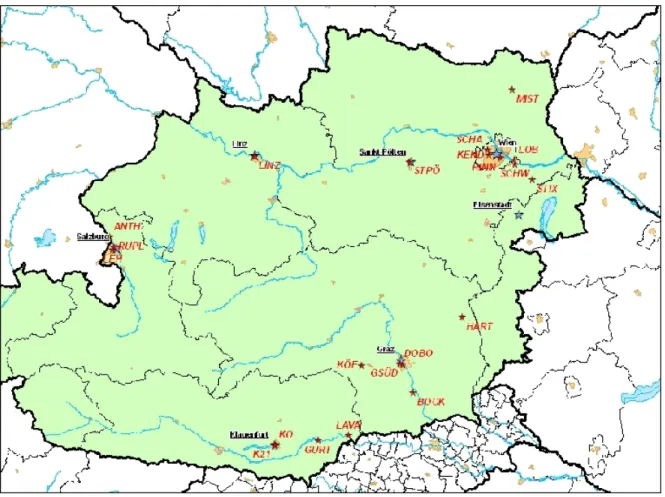
8.7 CARBOSOL - Pollen at PDD . . . III-21 8.8 CARBOSOL - Sugars contribution to OC . . . III-24 9.1 AQUELLA - Levoglucosan . . . III-28 9.2 AQUELLA - Mannosan . . . III-29 9.3 AQUELLA - Galactosan . . . III-29 9.4 AQUELLA - WS to PM . . . III-32 9.5 AQUELLA - Cellulose . . . III-40 9.6 AQUELLA - Plant debris contribution to PM10 . . . III-41

(22)

Part I

(23)

Chapter 1

Background and goals

Air pollution results in poor air quality that can affect the entire population. Epidemiological studies and tragical episodes have shown that, though the scientific basis is somehow still unclear, a raise in ambient atmospheric particulate matter (PM) concentrations leads to an increase in morbidity and mortality [1]. Also, particulate matter has effects on the climate, through both direct and indirect effects. At the present time, aerosols are a major uncertainty in the modelling of the future global climate. [2]

These public health concerns have lead policy makers towards the adoption of more strin-gent standards. However, these limits have recently been violated in many European cities [3, 4]. In order to reduce PM concentrations, knowledge about the magnitude of individual source contributions is required. Emission inventories may help to understand the relative contribution of primary emissions, but large contributions from fugitive sources as well as from secondary formed aerosol are generally not accounted for in emission inventories. Therefore, methods based on the analysis of ambient PM combined with the analysis of PM from dif-ferent sources have emerged (e.g. [5]) These techniques are called receptor models. To apply them, one needs not to measure the PM emission of each source and know the subsequent dispersion in order to estimate the exposure at a given location, as it would be using the emission inventory approach. Instead, the chemical composition of the aerosol collected at the exposure location is partially determined, and from that point the contribution of a set of sources is estimated.

The goal of this work was to study the european aerosol saccharidic composition and, relating it to the source emission levels, assess the importance of the contribution of their sources to the PM ambient levels.

(24)

Chapter 2

The atmosphere

2.1 Evolution and composition of the atmosphere

After the solar system formation some 4.6 billion years ago, the earth’s very earliest atmo-sphere probably was swept into space by a strong stream of particles emitted by the sun, the solar wind. As the planet slowly cooled down, the molten surface solidified into a crust and volatile compounds were released in a process called outgassing. [6, 7]

The primordial earth’s atmosphere, thought to have resulted of the release of trapped volatile compounds from the planet itself, was most probably a mixture of gases as the ones that volcanoes release today: carbon dioxide (CO2), nitrogen (N2) and water vapour (H2O),

with small amounts of hydrogen (H2). [7] As the planet continued to cool, the water vapour

condensed and formed clouds, wich generated rains, accelerating the cooling of the planet and slowly forming oceans, thus reducing the presence of water vapour in the air, as well as CO2,

dissolved into the oceans and which formed sedimentary rock at their bottom. [6, 7] Being inert and insoluble in water, nitrogen accumulated to become today’s most abundant gas on earth. [7]

The first life-forms on earth, probably bacteria, appeared in a mildly reducing atmosphere. Through photosynthesis, in which sugars are synthesised from the atmosphere’s CO2with the

input energy of solar radiation, oxygen is realeased into the air as a by-product. This way, bacteria and their successors, plants, released the first oxygen into the air. This early oxygen first oxidised other substances dissolved in water, such as iron. Once these substances were almost fully oxidised, oxygen started to accumulate in the atmosphere and today’s level is maintained by a balance between photosynthesis (production) and decay of organic carbon (removal). [6, 7]

Today’s atmosphere is strongly oxidising. It is composed of the main gases: nitrogen (78%), oxygen (20%) and argon (1%); water vapour (highly variable content, up to 3%), and trace gases such as ozone, carbon dioxide, neon, helium, methane, krypton, hydrogen and many more. [6, 7] The atmosphere also comprises aerosols (particles) [7].

(25)

Table 2.1: The composition of the atmosphere includes major and minor (trace) gases [6] main gases N2 abundance controled over geologic time scales

O2 biosphere, crustal material

Ar degassing of planet’s interior

vapour H2O highly variable

trace gases CO2 important for radiative balance

Ne

CH4 mole fraction <106, important for radiative balance

Kr < 1% of the atmosphere

H2 originate from geological, biological,

He chemical and anthropogenic processes

2.2 Height and structure of the atmosphere

2.2.1 Altitudinal variations in temperature

Regarding to temperature, the atmosphere can be divided into four major altitudinal zones. Within those zones, temperature increases or decreases with altitude depending on the exis-tence of heat sources.

The bottom layer stretches from the sea level up to an altitude of 9 to 16 km and is called the troposphere. The height of the tropopause depends on the latitude, with the polar tropopause lying at the lower end of the range and the tropical one at its maximum. Surface temperatures (the heat source) and the consequent thermal mixing are responsible for this difference. [6] The troposphere is characterised by a good transfer of atmospheric properties by large-scale turbulence and mixing.

Above the tropopause lies the stratosphere. Between the tropopause and a height of about 20 km, the temperature remains almost constant. From that height up to the tropopause (about 50 km above the earth’s surface), temperature increases with altitude. Ozone absorb-ing solar ultraviolet radiation is the heat source at the stratopopause. [6] Characteristic of the stratosphere is a poor vertical mixing. [7]

The third thermal layer of the atmosphere is the mesosphere, stretching from the stratopause to the mesopause (about 80 km of altitude), where temperature again decreases. This layer is characterised by good vertical mixing. [7]

The thermosphere, the fourth and last thermal layer, contains only a very small fraction of the atmospheric mass. Within that layer, the temperature increases, with the absorption of very short wave, high energy, solar radiation by ozone and azote atoms. The gas atoms and molecules of the thermosphere move very quickly, having a high temperature. However, being the thermosphere so depleted, the collective quantity of heat of the gases is very low. [6]

2.2.2 Altitudinal variations in composition

The atmosphere can be divided into two vertical layers in view of its composition: the ho-mosphere and the heterosphere. The lower layer, the hoho-mosphere, streches up to 80 km in altitude and is characterised by an uniform makeup of its component gases. The upper layer

(26)

is instead heterogenous in its vertical composition: the heterosphere. It can be subdivided into four layers, from bottom up, these are dominated by azote, atomic oxygen, atomic helium and atomic hydrogen. This layering has to do with the different strength of gravity upon the different molecules or atoms. [6]

Between roughly 80 and 400 km, azote molecules and oxygen atoms are readily ionised due to the absorbtion of short wave, high energy, solar radiation. This electrically charged portion of the atmosphere is known as the ionosphere. [6]

2.3 The radiative balance of the earth-atmosphere system

The driving force of the earth’s climate is absorption of solar radiation at the surface and, to a lesser extent, by the atmosphere. Absorption of solar radiation of course results in heating of the system. As the temperature of the system increases, it emits increasing amounts of thermal infrared radiation. The absorption of solar (shortwave) radiation by the earth-atmosphere system is approximately balanced by emission of thermal infrared (longwave) radiation, so that the earth may be considered to be in radiative equilibrium – more accurately, steady state – at least in global and annual average. [8]

Radiative forcings (RF) are changes in the energy fluxes of solar radiation (maximum intensity in the spectral range of visible light) and terrestrial radiation (maximum intensity in the infrared spectral range) in the atmosphere induced by anthropogenic or natural changes in atmospheric composition, earth surface properties, or solar activity. [2] Anthropogenic contributions to the chemical composition of the atmosphere affect the balance of both visible and infrared radiation of the earth-atmosphere system [9]. The first examinations of climate change addresses heat-trapping or ”greenhouse” gases such as CO2. This greenhouse effect

is the best known and most targeted for mitigation. The opposite effect of ”atmospheric cooling” is provided by increases in scattering or reflective aerosols, primary sulphates. While particles of any composition reflect light back to space, only a few can absorb light. These include black carbon or ”soot”, desert dust and some organic carbon species.

Also, particulate matter has the ability to alter the hydrological cycle and thus indirectly introduce a RF.

(27)

Chapter 3

The atmospheric aerosol

The many microscopic particles (aerodynamic diameter (a.d.) between 0.001 and 100 µm) that remain suspended for considerable periods of time are called aerosols. They originate from many sources, both natural and anthropogenic, and include sea salts from breaking waves, fine soil blown into the air, smoke and soot from fires, pollens and microorganisms lifted by the wind, ash and dust from volcanic eruptions and many more. [6] Some of these particles are solids, by-products of combustion, or incombustible matter; whereas others are secondary aerosols such as sulphate and nitrate species or semi-volatile organic compounds (SVOCs) [10]. Aerosols are most numerous in the lower atmosphere near their source, the earth’s surface. Particles present in the upper atmosphere are either carried from the lower atmosphere by rising currents or originate in desintegrated meteroids. [6]

These particles can act as surfaces on which water vapour may condense, contributing to the formation of clouds and fogs. They alter the radiative balance of the earth by absorbing or scattering solar light. They affect the oceans, soils and plants, human health and the build environment.

The aerosol of the lower atmosphere, the troposphere, is the focus of this work.

3.1 Physical characteristics of the tropospheric aerosol

3.1.1 The aerodynamic diameter

Aerosol particles have all kinds of shapes. Usually, these shapes are normalised to the diameter of a sphere with the same aerodynamical properties. The particles can then be characterised by their aerodynamical diameter, a.d. PMx means particulate matter with a.d. below xµm.

[7] However, the particles’ unregular shapes and sampling limitations makes it impossible to have a well-defined a.d. below which particles are collected and above wich they are not. Therefore, a PMx sampler is defined as a sampler that has 50 % collection efficiency for

particles with a.d. < xµm.

3.1.2 Particle formation pathways

Friction and abrasion Mechanical processes (friction and abrasion) are preponderant in the formation of larger particles. These processes may occur between two solid surfaces (e.g. tyre wear abrasion) or between a solid/liquid surface and the wind driven atmosphere as a fluid (e.g. sea salt: interface between the sea and the atmosphere; soil dust: interface

(28)

between the soil surface and the atmosphere). These particles may also grow secondarily through condensation and coagulation processes.

Nucleation Nucleation plays a fundamental role whenever a phase transition (condensa-tion, precipita(condensa-tion, boiling, ...) occurs. Four types of nucleation processes can be distin-guished:

Homogeneous-homomolecular: self-nucleation of a single species. No foreign nuclei or surfaces involveed.

Homogeneous-heteromolecular: self-nucleation of two or more species, without the par-ticipation of foreign nuclei or surfaces.

Heterogeneous-homomolecular: nucleation of a single species on a foreign nuclei or sur-face.

Heterogeneous-heteromolecular: nucleation of a more than one species on foreign sub-stance.

[7, 11]

The formation of water droplets in the atmosphere is the most evident example of nu-cleation. This reaction occurs much more readily when it is heterogeneous, and the nuclei are called cloud condensation nuclei (CCN). Also, foreign nuclei are needed for the water to freeze at 0◦C. Without these nuclei (ions or particles), which act as ice cristals nuclei, the freezing point would be lower. Besides the ice cristals and water droplets, nucleation of trace substances from the vapour phase to the solid (droplet) phase is of interest in atmospheric science. This step is fundamental in the formation of secondary aerosol, defined as the gas-to-particle conversion of vapours: trace gases emitted at high temperature readily condense when cooled in the atmosphere. Organic vapours may undergo such processes. Also, the reaction products of inorganic gases (SO2, NH3, NOx) and other pollutants (e.g. OH, O3)

may suffer homogeneous nucleation. Once the inicial nucleation step occurs, the nuclei of the new phase grows rapidly through condensation of gases onto its surface. Coagulation of more than one of these particles also leads to their growth. [7, 11]

3.1.3 The size distribution function

The atmosphere over all kind of areas contains significant amounts of aerosols, up to 107_–

108 cm−3. Their size (a.d.) spans over four orders of magnitude, from a few nanometers to around 100 µm. The particle size affects both atmospheric lifetime and chemical and physical properties. The division of the particle size range into discrete intervals and the accounting of the number of particles in each size bin leads to a size distribution. It is common to normalise the distribution by dividing the concentration by the respective size range (the concentration is then expressed in µm−1 cm−1). When the size bin is shortened to the limit (0), one reaches a continuous distribution. This can be done not only with particle number (as illustrated till here) – the number distribution – but also with particle surface area, volume and mass – the surface area, volume and mass distributions, respectively. For convenience, the aerosol a.d. is often log or lognormal transformed. [7]

The most used size distribution function is the mass distribution function. It evidences that the aerosol usually has 2 or 3 modes: one or two smaller modes, with maxima below

(29)

1 and around 1 µm, the nucleation and accumulation modes; and one coarse mode, with a maximum above 1 µm. The nucleation and accumulation modes are denoted as fine particles, a.d. below 1 µm (2.5 µm for some authors, mainly in a health effects perspective). The nucleation mode particles are formed by nucleation processes, while the accumulation mode ones are formed by condensation and/or coagulation processes involving nucleation mode particles or accumulation mode particles. [12, 7, 11, 13] Coarse particles are formed mainly by friction and abrasion processes. Though, some secondary particles may be found in this mode, mainly from the condensation of vapours into existing particles. [7]

3.2 Sources and production mechanisms of the tropospheric

aerosol

There are plentiful sources of atmospheric aerosols, which cover a very broad range of size distributions and other physical properties as well as chemical characteristics. In the following sections, the principal aerosol sources are reviewed and their fluxes, effects and main physical and chemical characteristics are briefly described. In regard to their origin, aerosols may be: Primary: directly emitted to the atmosphere. Formed by mechanical processes, mainly

coarse. These particles retain much of the chemical properties of their sources.

Secondary: formed by gas-to-particle conversions through chemical reactions (by nucleation and further coagulation and condensation processes). These particles may undergo great chemical changes.

Anthropogenic: formed by human activities. Biogenic: formed as a result of ecological activity.

Two kind of mixings can be distinguished:

external mixing: different sorts of particles (origin, composition, ...) are mixed inside a plume.

internal mixing: the individual particles of a plume contain different kind of origins and compositions.

In the following subsections, the main sources of PM are described, their origin mecha-nisms, their physical properties, their fluxes, their effects and briefly their chemical charac-teristics. For the purpose of this work, greater emphasis is given to primary aerosol, namely primary biological aerosol and biomass burning aerosol.

3.2.1 Soil and road dust

Dust are primary particles resulting from the friction of a fluid (the wind) with a solid (the earth’s crust). Its sources may be natural and anthropogenic [14]. The atmospheric lifetime of dust depends on the particle size: the larger the particle, the shorter its atmospheric residence time (submicron particles may have atmospheric lifetimes up to several weeks). Dust is characteristically < 100µm a. d., most of it is coarse aerosol [7, 15, 16] and is mainly composed of mineral material, such as Si, Ca, Mg, Al and Fe [7]. However, processes leading to its emission, involving wind, may also resuspend some primary biological material. [17]

(30)

Natural dust sources are mainly deserts, dry lake beds and semi-arid desert fringes [15, 16]. The Saharan sources are considered the most active (more specifically, the Bod´el´e depression in Chad), other major global sources are deserts in the Arabian Peninsula, Iran, Turkmenistan, Afghanistan, Pakistan and Northern India, the Tarim basin in China, the Namid and the Kalahari deserts in Southern Africa [14]. Dust deflation occurs in a source region when the wind speed at the surface exceeds the threshold velocity to lift deflatable material. [15, 14] This velocity is a function of surface roughness elements, grain size and soil moisture. It is thus dependent on the climatic conditions and varies in the range 5 –12.5 m s−1. [15, 14].

The wind speed at which deflation occurs is determinant for the aerosol number and mass distributions, which evolves with altitude and the time after the deflation [15], as observed by Xin et al. (2005) [18]. Typical volume median diameters of dust particles are of the order of 2 to 4 µm [15]. Chun et al. (2001) [19] observed shift towards larger size ranges in the aerosol number distribution in comparison to non-dust events. Levin et al. (2005) as cited by Kelly et al. [20] observed dust distributions with three modes at an elevation of about 500 m and high fine-dust number concentrations from the surface to altitudes up to and above 2000 m. Also, dust may get internally mixed with other types of aerosol (sea salt, sulphate, . . . ) [15, 18], thus affecting is size distribution and lifetime, as well as the characteristics relevant to its climate effect. [21, 22]

Human activities also contribute to the atmospheric dust budget and such impact may contribute significantly to regional dust emissions [14]. The ways in which humans can influ-ence dust emissions are:

• by land use which changes soil surface conditions that modify the potential for dust emission (e.g. by agriculture, mining, livestock, vehicles or water management)

• by modifying climate, which in turn modifies dust emissions, for example, by changes in surface winds or vegetation growth

• road dust and building activities are an anthropogenic input to the global dust budget [14]

Annual global dust emissions are estimated between 1000 and 3000 Tg. Of these, the Saharan contribution is estimated to 130 – 760 Tg yr−1 or even up to 1600 Tg yr−1 [14]. The highly uncertain estimation of the anthropogenic contribution to dust is evaluated to 0 – 50 % [14]. Satellite imagery and dust concentration measurements confirm that dust emitted from desert sources can be transported over large distances in the atmosphere affecting life, ecosystems and climate far from its origin (see 3.6.4) [14, 23]. However, only the smaller particles travel large distances, sometimes up to 5000 km [7].

Virtually any anthropogenic and biogenic source emissions to the urban atmosphere can, via atmospheric removal processes (e.g., dry deposition), contribute to the road dust compos-ite. This road dust can be resuspended into the atmosphere by the passing traffic or wind, followed by redeposition of some of that material back onto the streets. The main identified organic components of road dust, in the urban area of Los Angeles, were the same as for tyre wear: n-alkanes and n-alkanoic acids. [24]

3.2.2 Sea salt

Sea spray is generated by the process of breaking waves with direct sea spray emission or by a process which forms small sea water air bubbles. To become airborne, these bubbles might

(31)

be small enough, or a considerable part of their water content may evaporate. [7]

They cover a wide size range (approximately from 0.5 to 10µm), and have a correspond-ingly wide atmospheric lifetime. Their size distribution depends on numerous factors (among them is, given their hygroscopic nature, relative humidity) [15, 25] and is usually character-ized by three modes: the nuclei (a.d. < 0.1µm), the accumulation (a.d. between 0.1 and 0.6 µm) and the coarse (a.d. > 0.6µm) modes. The coarse mode typically comprises 95 % of the total mass but only 5 – 10 % of the total number. [7]

The total sea salt flux from the ocean to the atmosphere is estimated to be 3300Tg yr−1. [25] Estimates of relative contributions of dry and wet removal processes to total sea-salt removal vary largely, from roughly 70–33 % for wet and dry deposition, respectively, over open ocean to 30–70 % in the coastal zone and further down to 15–85 % on the continent. [26]

On a global scale, sea salt is important for aerosol effects on climate. [15, 27, 28] They are very efficient cloud condensation nuclei (CCN) and can directly supply more than 80 % of the cloud condensation nuclei in the marine boundary layer (MBL) when wind speeds are moderate and high (above 12 m s−1), especially for winter seasons over middle and high latitude regions. The secondary aerosol formation in the MBL due to oxidation of sulphur and nitrogen oxides also depends on sea spray. [29] On a regional scale, in places not far from the sea, they are important contributors to the aerosol loading, thus impacting human health, the natural and build environments, . . . [30, 31, 29, 26]

The chemical composition of aerosols originated in the sea is dominated by NaCl and sulphates (Na2SO4, MgSO4 and K2SO4).

3.2.3 Volcanic primary and secondary aerosols

Two components of volcanic emissions are of most significance for aerosols: primary dust and gaseous sulphur [15]. Also, other volcanic gases can be removed from the atmosphere by chemical reactions, wet and dry deposition and by adsorption onto volcanic ash [32].

Volcanic sources are important to the sulphate aerosol burden in the upper troposphere, where they might contribute to the formation of ice particles and lead to a change in the radiative balance of the earth-atmosphere system (see 3.4.4 and 2.3). Emissions from volcanoes that are strong enough to penetrate the stratosphere are rare. But due to their long lifetime they have a sensible effect on the climate. [15]

Volcanic dust fluxes into the atmosphere were quantified for the 1980s as ranging from 4 to 10000 Tg yr−1. The lower limit is representative of continuous eruptive emission while the upper limit represents large explosive eruptions. [15] Jaenicke [33] present a source strength of approximately 15–90 Tg yr−1 for volcanoes. Sulphur emissions occur mainly in the form of SO2, with minor amounts of SO2−4 aerosols and H2S. This sulphur is very important in

the formation of secondary aerosol. Historical records have shown that 100 Tg of SO2 can

be emitted in a single event (Tambora volcano eruption in 1815). Such large eruptions have lead to a strong transient cooling effect but there is no indication of any significant trend in the frequency of highly explosive volcanoes. Thus, while variations in volcanic activity may have influenced climate at decadal and shorter scales, it seems unlikely that trends in volcanic emissions could have played any role in establishing a longer-term temperature trend [34, 15], except maybe in catastrophical events that occur in hundreds or thousands of years.

Volcanic gases, such as acids and metal salts that adsorb onto volcanic aerosol during the eruption, dissolve within the hour when they come into contact with water, releasing

(32)

acids and metals in the environment. They cause the acidification and contamination of soils and surface waters, impacting seriously the vegetation, animals and people (e.g. half of the icelandic livestock perished due to fluorosis after the Laki eruption of 1783-84). [32] Volcanic ashes also have a fertilizing action on soils, and by increasing oceans primary productivity they enhance the sequestration of atmospheric carbon dioxide by the oceans [32].

Quiescent (non-explosive) degassing of volcanoes worldwide also inputs trace metals as aerosols to the atmosphere [35].

3.2.4 Primary and secondary biogenic aerosols

Primary biological aerosol particles (PBAPs) comprise material that originally derives from biological processes which was released into the atmosphere without change in its chemical composition. These particles may maintain their physical characteristics (pollen, spores, bacteria, viruses, algae, fungi, etc. . . ), specifically their cellular structure, or be the result of an abrasive process (fractionated material: plant or animal debris such as epithelial cells). [36] They are mainly in the aerosol coarse mode [7].

Some PBAPs are the cause of allergy-related diseases such as asthma, rhinitis, and atopic eczema [37]. They may be of importance for both direct and indirect climatic effects. The presence of humic-like substances makes this aerosol light-absorbing, especially in the UV-B region [15], and they are also able to act both as cloud droplet and ice nuclei [15, 36] and may play an important role for the long-range transport of trace elements into and away from specific biomes and in the spread of biological organisms and reproductive materials [38, 39]. Atmospheric PBAPs have been detected in various size ranges (e.g. PM0.2−2, PM>2, PM2.5

[40, 41, 42, 43, 44, 45, 38]).

Biological particles may, like aerosol particles of other origin (e.g. mineral dust, sea salt, biomass smoke, pollution particles, particles nucleated from gas phase emissions of many types), influence cloud formation and precipitation processes via the following paths:

• the phase change from vapour to liquid

• the acceleration of coalescence by large particles • the phase change from vapour or liquid to ice

In the second path listed above only the size, shape, and density of the particles are important. The other two processes depend on more specific properties, such as chemical composition. It may be pointed out that from what is presently known, ice nucleation by biological aerosol particles is expected to have the greatest potential of influence on cloud evolution by this class of particles. [46, 36]

In a study conducted in Germany, Despr´es and co-workers [38] found that most of the extracted DNA sequences in PM2.5 were from bacteria (mainly Proteobacteria). The authors

also found sequences from ascomycota and basidiomycota fungi, whose presence in the atmo-sphere had been reported by Elbert et al. (2007) [47], green plants and moss spores as well as one protist.

Very little is known about their contribution to aerosol mass, specifically PM10mass [15].

Among structural units, the largest PBAP particles are pollen. In the atmosphere, pollen are typically of a size of 30 µm and above, with a few exceptions (birch pollen) as small as 10 µm. Even as pollen can be carried over large distances, they generally tend to deposit due to their large size, thus high concentrations will be limited close to their emission sources. [37]

(33)

Allergenic material derived from pollen is known to also occur at smaller particle sizes, but only as a consequence of a fractionation process. [39]

Fungal spores, bacteria and viruses are clearly differentiated by their mass. The mass of spores is in the range of 33 pg (13 pgC/spore) [48]. Spores can be assumed to remain suspended in air for an extended period of time. Elbert and co-workers [47] estimated a global emission rate of total fungal spores of 50 Tg yr−1.

Bacteria have a mass about three orders of magnitude smaller (17 fg C [48]) than spores. Due to this vastly diminished mass, their contribution to total aerosol mass becomes negligible. The same is the case for viruses, to which far smaller mass has been attributed. They are not considered to occur as individual particles but instead to form clusters or droplets. [39]

Quantification of fractionated material is more difficult, as neither structure nor size are well defined. Matthias-Maser and co-workers [45] used protein as a tracer compound for a general quantification of PBAP, while Kunit and Puxbaum [49] developed a method to determine cellulose, a compound contained in fractionated plant tissue or plant debris, also occurring in fractionated pollen. Rogge and co-workers [50] indicated n-alkanes, n-alkanals, n-alkanols and aliphatic acids as the main organic groups present in green and dead leaf abrasion products.

Vegetation emits large amounts of reactive carbon to the atmosphere [51]. Secondary bio-genic aerosols are formed in the atmosphere by the mass transfer (condensation processes) to the aerosol phase of low vapor pressure products of the oxidation of volatile organic compounds (BVOCs). [7, 52, 51] These biogenic organic gases are dimethylsulfide (DMS) produced by phytoplankton, monoterpenes produced by forests or other BVOCs, though less important. [7, 52] Recently, photo-oxidation products of isoprene have also been reported as sources of secondary biogenic aerosol. [53, 54, 55, 56]

The total global biogenic (primary and secondary) organic emissions are estimated to range from 491 to 1150 Tg yr−1, exceeding the estimated anthropogenic emissions by as much as an order of magnitude [57].

Subsection 3.4.3 deals with the chemical precursors and the origins of biogenic secondary organic aerosol (SOAb), while subsection 3.5.3 refers to the end compounds observed in

am-bient aerosol.

3.2.5 Primary and secondary anthropogenic aerosols

Transportation, coal and biomass combustion, cement manufacturing, metallurgy and waste incineration are among the industrial and technical activities that produce primary aerosols [15]. These have been widely monitored and regulated in recent years in developed countries, where, as a result, air quality has improved. However, fast-growing industrialisation in de-veloping countries may lead to increases of these sources to values above 300Tg yr−1 by 2040 [15].

These aerosols cover a very wide range of size distributions and are mainly found in urban and suburban areas, where the anthropogenic activities have greater expression. However, they can be transported to remote sites. The differentiation of the quantification of various sources can be done with chemical analysis of source specific tracer species.

This subsection describes the main anthropogenic aerosol sources. Due to the scope of this work, greater emphasis is given to biomass burning, more particularly wood burning.

(34)

Industry, metallurgy, extraction industry and cement and ceramics manufactur-ing

Industry is a significant source of particulate matter in the atmosphere. The industry type and the used technology, the raw materials, the localisation and the abatement strategies used are factors that make the aerosol from those source highly variable in chemical composition, physical properties and fluxes. For example, the main components for a steel sintering plant, a cement plant and a foundry plant are:

steel sintering plant: Fe2O3 and K2O

cement plant: CaO and SiO2

foundry plant: SiO2, with minor amounts of Fe2O3 and Al2O3

[58]

Construction, demolition, quarries, mining, . . . are a source of generally coarse aerosols. The generation of aerosol by those activities, their chemical and physical characteristics de-pend on the mechanical activity, the raw material composition and wind speed.

Cement and ceramics manufacturing also produce mainly coarse aerosol.

It is difficult to asses the properties of such particulates due to their resemblance to soil dust.

Traffic sources

Traffic aerosol may arise from fossil fuel (mainly gasoline and diesel) combustion, tyre or break wear. Traffic is also responsible for the resuspension of road dust (see 3.2.1). Also, the gases produced by the evaporation of fossil fuels or their combustion taking place in the internal combustion engine can produce secondary aerosol (see 3.4.3, 3.4.4). Generally, diesel engines produce a greater number and mass of aerosols than gasoline engines.

Passenger cars, light- and heavy-duty vehicles, mopeds and motorcycles all contribute to the atmospheric aerosol burden. Particulate emissions in the vehicle exhaust mainly fall in the PM2.5 size range. The aerosol produced by the combustion engine are dominated by fine

aerosols and trace species such as Zn, Mo, Ni, Cu, Ag, Cd, Sb, Br, Se, dioxins, furans, PAHs and carbonaceous aerosols are emitted. [59, 60, 61, 62, 63, 64] Also, the nitrogen, sulphur and volatile organic species associated with this source are very active in the formation of the secondary aerosol. The emission factor and particle physical and chemical characteristics of exhaust particulate matter are highly dependent on the vehicles velocity, the engine condition (cold or hot), its maintainance, the driver’s behaviour and altitude. However, emission factors per mass of fuel are very similar among vehicle classes. [9, 62]

Tyre material is a complex rubber blend, although the exact composition of the tyres on the market is not usually published for commercial reasons. Tyre tread wear is a complex physicho-chemical process which is driven by the frictional energy developed at the interface between the tread and the pavement aggregate particles. Tyre wear particles and road surface wear particles are therefore inextricably linked. The actual tyre wear abbrasion rate depends on a large number of factors, including driving style, tyre position, vehicle traction configu-ration, bulk surface material properties, tyre and road condition, tyre age, road surface age, and the weather. [62]. The abbrasion of tyre wear produces more coarse aerosol, but an appreciable part (around 20% of the total particles emitted) are below 1 µm a.d. Estimates

(35)

of emissions range from 16 to 120 mg per vehicle-km, most of it being carbonaceous material [62]. n-Alkanes and n-alkanoic acids were the major identified organic classes in Los Angeles road dust and tyre wear. [24]

In breaks, linings generally consist of four main components – binders, fibres, fillers, and friction modifiers – which are stable at high temperatures. Various modified phenol-formaldehyde resins are used as the binders. Fibres can be classified as metallic, mineral, ceramic or aramide, and include steel, copper, brass, potassium titanate, glass, asbestos, organic material, and Kevlar. Fillers tend to be low-cost materials such as barium and antimony sulphate, kaolinite clays, magnesium and chromium oxides, and metal powders. Friction modifiers can be of inorganic, organic, or metallic composition. Graphite is a major modifier used to influence friction, but other modifiers include cashew dust, ground rubber, and carbon black. Break pads including asbestos fibres have now been totally removed from the European fleet. Estimates of emissions range from 8.8 to 84 mg per vehicle-km. The lower end of the range is typical for small passenger cars, while the upper end is representative for heavy vehicles. [62] The main identified organics in break lining wear by Rogge and co-workers [24] were n-alkanoic acids and polyglycol ethers.

For the EU15, the total exhaust and non-exhaust particles emissions, including roadwear abbrasion, of the road transport source is estimated to 338.1 and 298.4 kt of PM10 and

PM2.5, respectively. The non-exhaust sources account for 63.1 and 23.9 kt of PM10 and

PM2.5, respectively, including roadwear abrasion. [62]

Other traffic sources are off-road vehicles and aviation, shipping has also, recently, been pointed as a source of aerosol. [9, 65, 66]

Fossil fuel combustion – coal, fuel oil and gas

Particulate emissions, their physical and chemical characteristics, from solid fuel burning facilities vary geatly with the size of the facility because different combustion and abatement techniques are applied. In general, smaller facilities will emit more material (per unit of energy input) than larger ones. [10, 62]

The use of coal has diminished in the developed countries, and, in Europe, this source is significant only in some northern areas.

The chemical and physical nature of particulate emissions from coal-fired powerplants are considered to change considerably after emission into the atmosphere, varying with factors such as location, temperature, humidity and the presence of other pollutants [10].

When burning betuminous coal, the initial burning phase is dominated by the combustion of devolatilised organic matter. It is possible that uppon adding coal chunks to the fire, the chunks become hot enough for the devolatilisation to occur but not for their combustion (lukewarm ignition). [67]

Pulverised coal fly-ash aerosol leaving an electrostatic precipitator size distributions ap-pear to possess three distinct modes. These include a coarse fragmentation mode with par-ticle diameters greater than 5 µm, a fine fragmentation mode with diameters between 0.5 and 5 µm, and a ultrafine vaporisation mode: particles with diameters less than 0.5 µm. Fine and coarse fractions are formed by fragmentation, wheras ultrafine coal fly-ash parti-cles (a.d. < 0.5µm) are formed primarily through ash vaporisation nucleation and coagula-tion/condensation mechanisms. [68, 69]

The composition of the coal combustion aerosol is dependent on the appliance used. Mod-ern energy producing units will emit mainly mineral material that is not burnable. Units

(36)

without abatement technologies and not as efficient as thermo-electrical power plants emit also carbonaceous material (both BC and OC). Submicron and ultrafine coal fly-ash particles typically contain a large number of alkali and alkaline earth metals (Na, K, Mg, Ca) and transition metals (Ti, Mn, Fe, Co, Ni, Zn, V, Cr, Cu), and can be enriched in a number of metalloids and other trace elements including Sb, As, Se, S, and Cl. Non-volatile species such as Si are also found in the ultrafine fraction; carbon, probably soot originating from coal tar volatiles, has also been reported to be enriched in submicron particles. The amount of C depends on coal type and combustion device. [68, 69]

The other two modes, fine and coarse, originating from fragmentation, have a composition more similar to the original material, and soot, SiO2 and Al2O3 are the main components.

The SO2 emissions resulting from coal combustion are very important in the inorganic

secondary aerosol formation (see 3.4.4). Secondary sulphates are, in terms of mass, the proeminant aerosol emitted from coal-fired power plants. [10]

Fuel oil, and principally natural gas, are considered much cleaner fuels for power plants than coal. Their growing implementation as energy source worldwide is an important contrib-utor to the improvement of air quality. Fuel oil combustion is considered the major source of atmospheric V and Ni. [70] Of the identified organic classes, n-alkanoic acids were the most abundants, followed by n-alkanes and chloro-organics with smaller amounts of aromatic acids, PAH and oxy-PAH.

PAH and oxy-PAH were the major organic classes identified by Rogge et al. [71] for gas combustion, with minor amounts of n-alkanes and n-alkanoic acids.

Biomass combustion

Biomass burning has been used since pre-historic times for many purposes: clearing of forests and brushlands for agricultural use, control of pests and weeds, prevention of litter accu-mulation to preserve pastures, production of charcoal, cooking and room heating, aesthetic reasons, waste disposal, cooking animal feed, celebration and rituals, among others. [72, 9, 67]. Biomass burning also occurs for natural reasons (e.g. wildfires). [72]

Biofuels may be agricultural waste, animal waste or charcoal, but the main biomass burned is wood. [9, 67] There is a large uncertainty in quantifying biofuel use (and hence its emissions) inherent in the nature of the system. Wood and other biofuels are usually part of a complex system that meets a multiplicity of needs (animal fodder, building material, energy require-ments). [9] Wood typically consists of various lignins (20–30% dry weight), holocellulose (cellulose and hemicellulose, 40–50% and 20–30% dry weight, respectively) and extraneous compounds [73]. Cellulose provides a supporting mesh reinforced by lignin polymers. [67] On a regional scale, types of fuel used vary seasonally according to availability; within a household, constraints such as land tenure, animal ownership and storage space are of inter-est. [9] Softwood (pines, spruces, larches and firs) are prolific resin producers and comprise longitudinal wood fibers (or tracheids) and transversal ray cells. Softwoods lack vessel ele-ments for water transport that hardwoods have; these vessels manifest in hardwoods as pores. In softwood water transport within the tree is via the tracheids only. Besides these major components, wood tissues undergo photochemical degradation during wood weathering and yield organic acids, vanillin, syringaldehyde and other water-soluble high-molecular weight compounds. [67]

As a result of the processes during burning, biomass smoke contains a host of unaltered and thermally altered biomarker compounds from major vegetation taxa in the carbon number

(37)

range C8–C31 [67]. The major compounds giving rise to tracers upon burning are:

Lignin is present only in woody plants and is the main biopolymer in wood. It is a complex biopolymer with both aliphatic and aromatic constituents. Its main monomers are cinnamyl alcohols, either sinapyl alcohol (angiosperms – hardwood), coniferyl alcohol (gymnosperms – softwood) or p-coumaryl alcohol (gramineae – grasses).

Lignans are dimers of sinapyl , coniferyl or p-coumaryl alcohol contained in many wood tissues. They serve as toxins, supportive fillers or for other purposes.

Diterpenoids are resin acids such as abietic or pimaric acids synthesised mainly by conifers (gymnosperms – softwood) in temperate regions.

Cellulose is present in all plants. Cellulose molecules are linear polymers of 7000–12000 D-glucose units, forming bundles organised into parallel fibrous structures that support the wood tissue.

Hemicellulose is a mixture of polysaccharides formed by 100–200 units of glucose, mannose, galactose, xylose, arabinose, 4-o-methylglucoronic acid and galacturonic acid. There is a wide variation among wood species.

Sterols are produced by the biota in the carbon number range C25–C30. In higher plants,

β-sitosterol is the main sterol.

PAHs originally present in wood can also produce markers upon burning. [74, 75, 76, 67, 17].

There are several types of biomass burning:

Fireplaces and heating stoves are the only wood-burning appliances, used for space heat-ing and aesthetic reasons, when other energy sources (electricity, natural gas) are avail-able for cooking. Typically wood is burned in large pieces and the fire is untended. Type of wood, fuel loading, heat release and sap, ash and moisture content affect the total emission.

Boilers burn wood for building heat. They are common in Europe but not so in the U.S. Wood and vegetal waste are also burned for heat and power in industry, mainly in developing countries. In developed countries, industrial combustion of biomass (district heating, electrical production . . . ) is expected to have a small impact in the aerosol budget due to the use of abatement technologies.

Cooking: wood and other fuels are burned, mainly in developing countries for cooking and heating as well as a range of other applications. Efficiency, including exhaust design, is a key factor in PM emission. A fire optimised for heat transfer (usually where wood is scarce and its acquisition is ressources consuming) may remain in the flaming- and glowing-combustion mode longer than fireplaces or open burning. Total PM (expressed as g of PM per kg of fuel) emitted from cooking fire has been reported as low as those from fireplaces or stoves. Besides wood, agricultural waste (vegetal residues or animal dung, depending on availability, production and suitability for other purposes) may be used as fuel.

(38)

Table 3.1: Estimates for the global burned biomass.

Source Emission

tropical FC 500–1000 TgC yr−1 [67]

tropical SBC 300–1600 TgC yr−1 [67]

RB and cooking (including dung and crop residues) 600–1200 TgC yr−1 [67]

AF – firewood 300–600 TgC yr−1 [67] AF – agricultural waste 300–600 TgC yr−1 [67] WF – firewood 150–300 TgC yr−1 [67] savanna 3752 Tg yr−1 [9] forest 1939 Tg yr−1 [9] Agricultural residue 475 Tg yr−1 [9]

Bond et al. [9] gave data in Tg dry biomass, Gelencs´er et al. [67] gave data in TgC dry biomass.

Charcoal is often used in urban areas for being a cleaner fuel. The charcoal fuel cycle emits particulates at two stages: manufacture and use.

Open burning emissions depends on many factors that are specific to location and season, such as fuel moisture content. Open burning (OB) englobes wildfires (WF) (savanna fires, tropical or temperate forest fires, . . . ), forest (FC) and savanna/brushlands clear-ing (SBC) as well as the burnclear-ing of large agricultural residues (agricultural fires – AF). Forest and savanna fires occur for many reasons and in very distinct places, where the vegetation cover (the fuel), varies a lot. Agricultural fires are an inexpensive means to advance crop rotation and control insects, diseases and invasive species.

[72, 77, 9, 67, 78, 79], refer to Table 3.1.

Though not yet fully resolved, there are studies showing that the molecular signatures of these different fires are distinct. The small combustion sources, mainly residential burning (RB) but also smaller AF, are so numerous that they have a significan impact. [77, 67]

(39)

T able 3.2: Con trib ution (as %) of Biomass Smok e to PM compiled from recen t stud ie s. con tribution con tribution metho d to OM / to OC a (%) to PM (%) used reference alpine v alley da ytime 77 14 C as tracer and [80] win ter nigh ttime 90 m ulti-λ absoprtion tec hnique [81] South California, US a v erage 1982 PM 2 7–26 1.4–10.5 CMB (organic comp ounds) [5] S. Joaquin v alley , US residen tial/industrial 17–49 CMB (organic comp ounds) [82] win ter 1995, fine particles remote 0. 6 Southeastern US PM 2 .5 25–66 56–80, win ter CMB (organic comp ounds) [83] CMB: chemical mass balance

(40)

The process of biomass burning The first step in biomass burning, drying/distillation, releases water (capillary water first and then the bound water stored in cell walls) and volatile species. The next step, pyrolysis, forms char (portion of carbon that never leaves the original fuel particle – charring removes hydrogen and oxygen, so that char is composed primarily of carbon) of high carbon content, tar of intermediate molecular weight and volatile compounds in the form of a flammable white smoke. Above 450K the process is exothermic and at about 800K glowing combustion releases tar and gaseous products. These substances (tar and volatiles) are dilluted in an oxydising atmosphere (usually air) and ignite, forming a flaming combustion. Smouldering takes over when the supply of volatile speces in the near-surface of the fuel lessen. At this stage, usually under 850K, a vast amount of partially oxydised pyrolysis products are emitted. Open vegetation fires are typically dynamic fires where all the stages of combustion are expected to happen simultaneous and sequentially. [67]

Formation of smoke particles Particle formation in the flaming fire phase begins with the creation of condensation nuclei (such as PAH) from ejected fuel gases (volatile compounds) as well as from a variety of ”soot-like” species. These original particles grow through chemical and coagulative processes and become condensation nuclei for other pyrolised species (volatile compounds), and may experience considerable growth. Further oxidation in the flame zone, with high enough temperatures (above 1100K), may subsequently reduce those particles in size. If insufficient oxygen is transported into the flame or if the temperature is not enough to complete oxidation, the particles may undergo a secondary condensation growth phase and be emitted in the form of smoke. In general, particles production increases with increasing flame size, lower amount of oxygen in the fuel and increased flame intensity (reduced oxygen transport to the fire). [79]

smouldering combustion begins when most of the volatiles have been expelled from the cellulose fuel. It is a surface process where oxygen diffuses to the surface and reacts exother-mically with carbon (T> 710K). Because PAHs tend to form at higher temperatures, the mass fraction of soot in smoke particles produced during the smouldering phase is extremely low, and particle formation may occur around other nuclei (condensation of volatilised organics on any available particles or surfaces). [79]

Biomass burning is one of the largest sources of accumulation mode particles globally, with approximately 90% of the emitted particles in the accumulation mode (a.d. < 1µm). [79] Coarse particles are not built during the combustion process; the residence times involved are insufficient for either building these particles or coagulating them from smaller ones. Rather, these particles are left over from large particles present at the start of combustion, although these initial particles may divide during the combustion process. Coarse particles may include both mineral matter or char. [9]

Several macroscopic variables affect the emissions from wood combustion: burning rate, type of wood, moisture content and fuel size are the main ones. [9]

Physical properties of fresh smoke particles Accumulation mode smoke particles ex-hibit a wide variety of shapes and morphologies: chain aggregates, solid irregulars and liq-uid/spherical shapes. This feature depends on various parameters: combustion efficiency (oxygen availability) and combustion phase, among others. Coarse mode particles (about 10% of smoke particles, in mass) have a typical diameter of 2–15µm. Giant ash particles may also be emitted, with a.d. up to 1 mm. They are usually generated by very intense fires and

(41)

consist not only of combustion-derived particles but also of small non-combustible matter on or around foliage in the fire zone entrained into the fire plume (e.g. soil particles). Because this coarse mode consists of ash, carbon aggregates, partially combusted foliage and soil particles, their shapes are very varied. The count median diameter (CMD) for fresh smoke particles is in the range 0.10–0.16 µm (centered at 0.13), while the volume median diameter (VMD) lays between 0.25 and 0.3 µm. Also, on account of their highly water soluble composition, fresh smoke particles can be very effective cloud condensation nuclei. The secondary production of soluble material during the aging process further enhances the particle hygroscopicity and CCN efficiency (see 3.2.5). [84, 78, 79]

Chemical properties of fresh smoke particles Smoke accumulation mode particles have three principal components: organic matter (OM), black carbon and trace inorganic materials (mostly Na, Mg, Si, S, Cl, K and Ca). In average, fresh smoke particles from WF are composed of 80% organic matter, 5–9% black carbon and 12–15% trace inorganic species. Though there are wide variations, some conclusions about the composition of WF smoke particles may be drawn:

• smouldering combustion, occurring after most of the fuel solids were expelled and at lower temperatures without flame pyrolysis where the combustion of OM could take place, has higher organic carbon (OC) contents.

• The black carbon content of the flaming phase smoke particles is lower and not as variable as for the smouldering phase.

• The ratio OM/OC is variable and uncertain, in general between 1.4 and 1.8 and higher. • water extraction efficiency for carbon is in the order of 40–80%, being mainly organic acids, alcohols and sugars. Other compound classes observed are PAHs, esters and alkanols.

• Trace inorganic species (about <10%) are dominated by alkali earths and halides. Potas-sium and chloride each account for 2–5%. Sulphur is present in the form of sulphate (about 1%). They can form from vaporisation of minerals and subsequent condensation or from bursting of mineral inclusions of the fuel. Unlike carbonaceous aerosols, mineral material cannot be eliminated from the flue gas by oxidation.

[85, 9, 79].

For AF, Hays et al. [78] found 42 and 84% of C in PM2.5 from wheat and rice straw

burns, respectively. K and Cl were much more present in wheat than in rice straw burns. The composision of particles emitted by RB depends in a very large scale on the fuel used, also on the appliance and the type of fire. Pine, eucalyptus and oak wood burning emit mainly lignin derived compounds, syringols, resin and n-alkanoic acids, but the amounts of each of these classes varies, indicating a difference in the composition of smoke particles between softwood and hardwood. [86, 87, 88] Of the carbonaceous species resolved, levoglucosan is by far the major compound identified.

Aging of smoke particles Various studies have shown that smoke aerosol can be trans-ported for long distances and impact distant and even remote regions. (e.g. [89, 90, 91, 92, 93]) During that transport, smoke particles undergo physical change and/or chemical evolution,