Measuring inequality of opportunity across EU-SILC countries : national and urban-rural perspectives

(1)

REM WORKING PAPER SERIES

Measuring inequality of opportunity across EU-SILC countries:

national and urban-rural perspectives

Zbigniew Mogila, Patricia C. Melo, José M. Gaspar

REM Working Paper 0135-2020

May 2020

REM – Research in Economics and Mathematics

Rua Miguel Lúpi 20, 1249-078 Lisboa,

Portugal

ISSN 2184-108X

Any opinions expressed are those of the authors and not those of REM. Short, up to two paragraphs can be cited provided that full credit is given to the authors.

(2)

REM – Research in Economics and Mathematics

Rua Miguel Lupi, 20 1249-078 LISBOA Portugal Telephone: +351 - 213 925 912 E-mail: rem@iseg.ulisboa.pt https://rem.rc.iseg.ulisboa.pt/ https://twitter.com/ResearchRem https://www.linkedin.com/company/researchrem/ https://www.facebook.com/researchrem/

(3)

1

Working Paper

Measuring inequality of opportunity across EU-SILC countries: national and urban-rural perspectives1

Zbigniew Mogila2_{, Patricia C. Melo}2_{, José M. Gaspar}3

Abstract

Inequality in individuals’ outcomes resulting from unequal access to opportunities due to differences in individual circumstances, such as family background and/or race, are generally considered to be unfair and ethically unacceptable. Since wealthier individuals and their families tend to live in more affluent areas and mingle with similar more affluent peers, the territorial distribution of inequality of opportunity may partially be viewed as a measure of the extent of spatial (in)justice. One of the ways governments can use to mitigate inequality of opportunity is to improve access to socially valued resources, e.g. education, health. If the spatial distribution of these resources is not equitable, or prevents equitable access to them, persistent or even growing differences in inequality of opportunity may arise. Improving the spatial distribution of socially valued resources can help individuals enhance their socioeconomic prospects, while also increasing the full utilization of territorial capital and, consequently, contribute to greater socioeconomic cohesion. This paper measures the extent of inequality of opportunity at the national level and by degree of urbanization for the countries covered in the survey European Union Statistics on Income and Living Conditions (EU-SILC). Emphasis on the degree of urbanization allows exploring whether large(r) cities can act as social elevators compared to smaller urban and rural areas. Using the EU-SILC data, we implement regression models to measure the percentage of the variation in individual’s labour income that is due to family background, namely, the education, occupation and activity status of parents, and household financial situation. Our results indicate substantial variation in inequality of opportunity ranging from 4% (Iceland) to 25% (Luxemburg). In addition, the distinction between more liberal economies and the rest of the countries is seen with the former

more income unequal, however, with the smaller impact of family-related factors on individual’s

income. Moreover, the findings suggest that cities, especially larger ones, do not seem to work as social elevators and may in fact benefit individuals with a better family background.

Keywords: income inequality, inequality of opportunity, EU-SILC microdata

JEL codes: D31, I24, D63, J62

1_{This article is part of the European Union's Horizon 2020 project RELOCAL - Resituating the Local in Cohesion and} Territorial Development, GA727097. We also acknowledge the financial support from Fundação para a Ciência e Tecnologia (FCT) through national funds UECE-UID/ECO/00436/2013, as well as UID/GES/00731/2019, PTDC/EGE-ECO/30080/2017, and CEECIND/02741/2017.

2_{ISEG – School of Economics and Management, Universidade de Lisboa and REM/UECE – Research Unit on Complexity} and Economics, Lisbon, Portugal. E-mail: zmogila@iseg.ulisboa.pt & pmelo@iseg.ulisboa.pt.

3_{CEGE – Research Centre in Management and Economics, Católica Porto Business School, Universidade Católica} Portuguesa, Porto, Portugal. E-mail: jgaspar@porto.ucp.pt.

(4)

2 1. Introduction

The concept of inequality of opportunity originates in the philosophical foundations laid down by Rawls (1971), Sen (1985), Dworkin (1981), Arneson (1989) and Cohen (1989). Their insights gave rise to the distinction between ethically acceptable and unacceptable sources of inequality. If inequalities in socioeconomic outcomes result from individuals’ own effort and merit (e.g. if they study more), it is fair and ethically acceptable that they should have better outcomes (e.g. a better job and/or pay). In contrast, if inequalities in socioeconomic outcomes result from individuals’ circumstances (e.g. family background, race), they are considered ethically unacceptable in the sense that they reflect individuals’ luck in having been born in wealthy family backgrounds with better socioeconomic prospects. In this sense, the problem is not so much the inequality in outcomes amongst individuals, but rather whether that inequality reflects inequality in the opportunities available to individuals with similar levels of effort and merit. However, evidence suggests that the later tends to perpetuate the former (e.g. Corak, 2013).

One of the dimensions of inequality of opportunity is its spatial distribution. Since wealthier individuals and their families tend to live in more affluent areas (i.e. spatial sorting) and mingle with similar peers (i.e. positive assortative matching), the territorial distribution of inequality of opportunity may partially be viewed as a measure of the extent of spatial (in)justice. One of the ways national and sub-national governments can use to offset inequality of opportunity is to improve access to socially valued resources, e.g. high-quality educational and vocational training institutions, health care. If the spatial distribution of these resources is not equitable, or prevents equitable access to them, persistent or even growing differences in inequality of opportunity may arise. Improving the spatial distribution of socially valued resources can help individuals enhance their socioeconomic prospects, while also increasing the full utilization of territorial capital and, consequently, contribute to greater socioeconomic cohesion. The role of redistributive measures needs to be also emphasised as the effective measures to level the filed in terms of individual’s access, for instance, to high-quality educational institutions.

The aim of this paper is to measure the extent of inequality of opportunity at the national level and by degree of urbanization for the countries covered in the survey European Union Statistics on Income and Living Conditions (EU-SILC). The ex-ante measure of inequality of opportunity is applied, i.e. inequality between groups sharing the same circumstances (Van de Gaer, 1993; Kranich, 1996; Peragine, 2004). Using the EU-SILC data, we implement regression models to estimate the percentage of the variation in individual labour income that is due to family background and circumstances at age 14, namely, the education, activity status of parents, occupation of father, and household financial situation. In addition, we apply the Shapley decomposition to estimate the relative importance of each circumstance variable or group of variables.

This paper contributes to the existing literature by analysing inequality of opportunity using a range of family background circumstances in two time periods, namely 2005 and 2011, reflected in the special EU-SILC modules on intergenerational mobility. To the best of our knowledge, this is the first research study on inequality of opportunity by degree of urbanization and allows us to explore whether large(r) cities can play a role of social elevators compared to smaller urban and rural areas. Our results indicate substantial variation in inequality of opportunity ranging from 4% (Iceland) to

25% (Luxemburg).In addition, the distinction between more liberal economies and the rest of the

(5)

family-3

related factors on individual’s income. Moreover, the findings suggest that cities, especially larger ones, do not seem to work as social elevators and may in fact benefit individuals with a better family background.

The structure of the paper is as follows. In the next section, we give a brief overview of the conceptual framework and previous studies of inequality of opportunity. Then, our empirical strategy and data are shown. We subsequently present and discuss the results from the regression models. The paper concludes with a summary of our findings.

2. Overview of relevant literature

2.1. Conceptual framework

In order to translate the distinction between ethically acceptable and unacceptable sources of inequality into empirical models, Roemer (1998) introduces the terms of effort and circumstances. They define the set of factors which are respectively influenced by individuals and beyond their control. Using these two categories, i.e. effort and circumstances, Roemer partitions a given population into types and tranches. Types are defined as groups of individuals sharing the same set of circumstances (e.g. family background, age, gender). Hence, outcomes of individuals within a specific type are assumed to be solely due to effort. Tranches, on the other hand, are referred to as parts of the population exerting the same effort regardless of circumstances. With these categories in mind, Roemer implicitly presents equality of opportunity as a state in which the outcomes of those belonging to the same tranche are equal.4_{This is called a strong definition (Ferreira and} Gignoux, 2011; Brunori, 2016) and corresponds to the ex-post approach to inequality of opportunity (Roemer, 1993; 1998; Fleurbaey, 2008). In this case, inequality of opportunity is identified by comparing and contrasting outcomes within tranches.

The ex-post approach to inequality of opportunity shows, however, serious methodological limitations, which are associated with sample sizes often too small to allow estimating type-specific distribution functions, especially when the number of types is large (Ferreira and Gignoux, 2011). In order to handle this problem, a ‘weak equality of opportunity’ criterion was specified giving rise to the ex-ante measure of inequality of opportunity. According to this approach, inequality of opportunity is equivalent to inequality between types, i.e. inequality between groups sharing the same circumstances (Van de Gaer, 1993; Kranich, 1996; Peragine, 2004). This facilitates considerably the procedure of measuring inequality of opportunity as it does not require the measurement of efforts and the comparisons of the same effort percentiles across various types of circumstances (Ferreira and Gignoux, 2011). In order to carry out the ex-ante procedure, one should construct a counterfactual distribution of outcome by removing within-type inequality.

The counterfactual distributions derived in both ex-post or ex-ante methods are generated as a result of either non-parametric or parametric calculation procedures. In the case of the former (Checchi and Peragine, 2010), the counterfactual distributions are built without any functional assumptions in mind. This approach, however, can encounter the barrier of the limited number of observations which make up each circumstance type and tranche. Consequently, it may imply small

4_{Roemer does not formulate explicitly the definition of inequality of opportunity. In his work, he aims at redistribution} that would equalize opportunities in a given society.

(6)

4

samples to obtain precise estimate counterfactual distributions, especially in the case of the ex-post approach (Brunori, 2016). Consequently, parametric measures are often preferred. Here, reduced form regression models are usually adopted to produce counterfactual distributions (e.g. Bourguignon et al., 2007 and Ferreira and Gignoux, 2011) for the relationship between the outcome of interest (i.e. the dependent variable) and the circumstances and efforts (i.e. explanatory

variables).5_{Since some of the circumstances are not observable, and thus cannot all be taken into}

account in the regression model, the measures of inequality of opportunity are merely lower-bound estimates (see Ferreira and Gignoux, 2011 following Brunori, 2016).

2.2. Overview of empirical studies

There are a series of research studies looking at inequality of opportunity. Brunori et al. (2013) present outcomes of eight studies carried out using the ex-ante approach – both in its

non-parametrical and non-parametrical variants.6_{It is clearly shown that factors beyond individuals’ control}

(e.g. family background, place of birth, gender, race) play an important role in determining overall inequality. However, their share in total inequality varies considerably across the 41 countries studied (from 2% in Norway to 34% in Guatemala). Caution should be, however, exercised when comparing and contrasting the results generated from various studies because they differ in the methods of building counterfactual distributions (e.g. parametric versus non-parametric), focus on different outcomes (e.g. income versus consumption) and control for a different set of circumstances as well as the number of circumstance types (Brunori et al., 2013).

There are also several studies using the ex-post approach to the measurement of inequality of opportunity. Salvi (2007) controls for circumstance variables such as family background, ethnicity and local infrastructure (e.g. presence of bus service and electric power in the village, number of secondary schools, etc.) to measure inequality of opportunity in consumption across Nepalese households, and finds that inequality is mainly driven by infrastructure and ethnicity rather than by family background. Bourguignon et al. (2007) measure the extent of inequality of opportunity in individual earnings in Brazil by controlling for the role of circumstances such as: parental education, father’s occupation, race, and region of birth. They also measure how circumstances affect earnings using three eﬀort variables, namely own education, migration out of hometown, and labour market status. The outcomes obtained show that 25% of overall earnings inequality is due to inequality of opportunity. This effect is composed of the direct effect of circumstances (60%) and the indirect effect of circumstances channelled through efforts (40%). They conclude that the circumstances that affect earnings inequality the most are those associated with family background.

The methodological differences between the ex-ante and ex-post approaches to measuring inequality of opportunity are reflected in significant differences in their outcomes. As Checchi et al. (2010) show in their EU-SILC-based analysis of 25 EU countries, the ex-post approach tends to generate greater values (from 16% to 45% of total income inequality) than the ex-ante approach (from 2.5% to 30% of total income inequality). The importance of both approaches is underlined as

5_{As efforts are partly determined by circumstances, in the reduced-form regression models they are presented as the} function of circumstances. Consequently, the outcome (e.g. income) is exclusively regressed on circumstances (Brunori, 2016).

6_{The studies are: Checchi et al. (2010); Ferreira and Gignoux (2011); Ferreira et al. (2011); Pistolesi (2009); Singh (2011);} Belhaj-Hassine (2012); Cogneau and Mesple-Somps (2008) and Piraino (2012).

(7)

5

providing two complementary angles to look at the problem of inequality of opportunity, i.e. “distances between social groups” (ex-ante approach) and “the individual income gaps due to

circumstances” (ex-post approach) (Checchi et al., 2010). On the basis of the two definitions and

using as circumstances individual’s gender, age, residential area and education as well as parental education and occupation, they identify three groups of countries: 1) the former communist countries (Hungary, Poland, Latvia and Estonia) and Portugal, which are characterized by intermediate levels of inequality of opportunity and greater values of overall inequality; 2) Norway, Sweden, Denmark, Finland, Slovenia and Slovak Republic with low levels of both total inequality and inequality of opportunity; and 3) the most of continental Europe showing moderate levels of total inequality along with relatively high levels of inequality of opportunity. The outcomes might suggest a significant impact of more egalitarian social welfare systems (e.g. prevailing in the Nordic countries and former centrally planned economies) on building more equal opportunities for individuals’ development.

In another study using both ex-ante and ex-post approaches, Checchi and Peragine (2010) use non-parametric techniques to estimate the extent to which earnings inequality in Italy is due to inequality of opportunity. Circumstance are approximated by parental education, whereas the relative position in the income distribution (e.g. quintile) is used as a proxy of efforts. In addition, the authors control for gender and regions (Centre-South and North). The results show that around 20% of overall income inequality in Italy is due to inequality of opportunity. This effect is stronger in the southern regions of Italy, particularly for women. Perez-Mayo (2019) also carry out a regional analysis of inequality of opportunity for Spain. Using parametric regression models and EU-SILC microdata for 2011, they analyse ex-ante inequality of opportunity in Spanish NUTS-2 regions by controlling for the role of circumstance variables referring to parental education and occupation, as well as household financial stress during childhood. The outcomes show that around 10% of income inequality in Spain is due to inequality of opportunity due to family background: father’s education alone explains nearly 25% of the impact of opportunity circumstances on children’s income. The regional-level analysis reveals wide heterogeneity in the extent of inequality of opportunity in determining total income inequality, ranging from 3% (Cantabria) to 33% (Extremadura).

Andreoli and Fusco (2017) carry out ex-ante and ex-post based analyses of inequality of opportunity using the EU-SILC datasets for 2005 and 2011 and 19 EU countries. They use the educational attainment of the father as the main circumstance factor in explaining labour income. The ex-post perspective shows that the Nordic countries, Germany, Austria, Belgium, France, Cyprus and the Netherlands are characterized by low inequality of opportunity (from 2.3% to 4%), whereas the remaining EU countries studied, mainly lower-income member states, show greater inequality of opportunity (from 4.3% to 9.8%). The ex-ante approach reveals a similar geographical pattern of inequality of opportunity. However, as in the case of Checchi et al (2010), the ex-ante measures are lower than the ex-post measures. In addition, they find no significant changes in the extent of

inequality of opportunity between 2005 and 2011.7

Although there is some evidence of inequality of opportunity at the regional level, we could not find any studies looking specifically at the extent of this phenomenon across the urban hierarchy and in particular between urban and rural areas. Since cities are often presented as “social elevators”, we

(8)

6

are interested in studying the difference in the degree of inequality of opportunity between urban and rural areas.

3. Data and methodology

3.1 Empirical strategy

From a theoretical point of view, both the ex-ante and ex-post approaches provide us with complementary perspectives when looking at the extent of inequality of opportunity. However, when it comes to their operationalization, the latter usually entails strong assumptions necessary to estimate efforts (Juárez and Soloaga, 2014). Unfortunately, the EU-SILC dataset that we use does not allow us to avoid those limitations regarding the estimation of the exerted efforts. We decide, thus, to follow the ex-ante approach to the estimation of inequality of opportunity, similarly to previous studies using the EU-SILC microdata (e.g. Perez-Mayo, 2019).

To this end, we set out to calculate the level of inequality of opportunity, measured by the following index (Ferreira and Gignoux, 2011):

𝜃𝑎 = 𝐸0({𝜇𝑖𝑘}) = 1 𝑁∑ 𝑙𝑜𝑔 𝜇 𝜇_𝑖𝑘 𝑁 𝑖=1 (1) where:

𝜃𝑎 - absolute index of inequality of opportunity,

𝐸₀ - mean logarithmic deviation (inequality measure),

{𝜇_𝑖𝑘} = (𝜇1,…,1 𝜇𝑛,…,1 𝜇𝑖𝐾, … , 𝜇𝑁𝐾) - counterfactual (“smoothed”) distribution of income with N individuals (i) and K types (k),

𝜇 - overall mean.

Following Ferreira and Gignoux (2011), we use the mean logarithmic deviation as the inequality measure for individual labour income.8_{The first step taken to calculate the index of absolute}

inequality of opportunity (1) is to construct the “smoothed” distribution ({𝜇_𝑖𝑘}). For this purpose,

each individual outcome within a type (𝑦_𝑖𝑘) is replaced with the type-specific mean (𝜇𝑘(𝑦)). Individual outcome y in our analysis corresponds to labour income. We approximate the “smoothed” distribution using a parametric approach drawing upon a reduced-form regression model (Ferreira and Gignoux, 2011), as follows:

𝑙𝑛𝑦 = 𝐶Ψ + ε (2)

8_{The mean logarithmic deviation is a member of the generalized entropy indices and satisfies the following axiomatic} properties: principle of population, scale invariance, normalization, within-type symmetry, within-type transfer insensitivity, between-type transfer principle as well as additive decomposability, i.e. path-independent decomposability. For more details about the axiomatic properties in question, see e.g. Ferreira and Gignoux (2011) or Cowell (1995).

(9)

7

where:

𝐶 – the set of circumstance variables,

Ψ – the parameters reflecting both the direct and indirect (via efforts) effects of circumstances on outcome y,

ε - the error term.

Using the OLS estimator, the “smoothed” distribution is given by:

𝜇̃ = exp [𝐶𝑖 𝑖Ψ̃ ] (3) where:

𝜇̃ - counterfactual “smoothed” distribution from the OLS regression model, _𝑖

Ψ̃ - parameter estimates from the OLS regression model.

Dividing 𝜃𝑎 by total income inequality (𝐸0(𝑦)), we obtain a relative measure of inequality of opportunity (𝜃𝑟):

𝜃_𝑟 = 𝐸0({𝜇𝑖

𝑘_})

𝐸0(𝑦) (4)

The models were estimated in STATA using the user-written command iop (Juárez and Soloaga, 2014) to assess ex-ante inequality of opportunity for labour income as a continuous variable with inherent scale as proposed by Ferreira and Gignoux (2011). In addition, we apply the Shapley decomposition, whereby inequality measures for all possible permutations of circumstances are first estimated and then the average marginal effect for each circumstance on the measure of inequality of opportunity is computed in order to estimate the relative importance of each circumstance variable or group of variables (Juárez and Soloaga, 2014).

3.2 Data sources and variables

The models are estimated using data from the special EU-SILC module on intergenerational mobility for 2005 and 2011. We carry out the estimation of inequality of opportunity indices at the national level for 18 countries (Finland, Cyprus, Iceland, Norway, Sweden, Slovenia, Belgium, Estonia, Ireland, Lithuania, Luxembourg, the Netherlands, Slovakia, Denmark, the United Kingdom, Germany, France

and Austria).9_{In addition, inequality of opportunity is measured by degree of urbanization (large}

9_{We selected those countries out of 26 countries for which EUSILC data are available for both analysed years: 2005 and} 2011. For Portugal, Greece, Latvia, Italy and Spain there were no data on gross income in 2005.In the case of three countries, namely the Czech Republic, Hungary and Poland, data on gross income took on very low values falling in question their credibility.

(10)

8

urban areas, small urban areas and rural areas).10_{We excluded the Netherlands and Slovenia from}

these analyses because they do not report data on degree of urbanization.

Following Andreoli and Fusco (2017) we use the annual gross employee cash or near cash income as an output variable for labour income. This is the monetary component of the compensation in cash payable by an employer to an employee including any social contributions and income taxes payable by an employee or by the employer on behalf of the employee. Likewise, we restrict our estimation sample to male individuals, aged between 16 and 65, who worked full time as an employee. In order to ensure comparability of the outcome variable across countries, gross income was converted into Purchasing Power Standard (PPS) using the Eurostat data on purchasing power parities.

To account for the presence of lower-end outliers in the distribution of labour income, we use data

on minimum wages from Eurostat11_{, which is calculated based on 12 monthly payments per year.}

We convert these minimum wages to PPS and remove all observations with gross labour income lower than the annual minimum wage. Since there is no minimum wage data available for Finland, Austria, Germany, Denmark, Cyprus, Iceland, Norway and Sweden, we exclude observations with

reported income lower than the 5th_{percentile for those countries’ wage distributions. In addition,}

following Van Kerm and Alperin (2013), we remove the upper-end outliers of the income

distribution by dropping values that are 25% higher than the 99th_percentile.

The circumstance variables (see equation (2)) essentially refer to individual’s family background – i.e., education of father; education of mother; activity status of father; activity status of mother; main occupation of father; and the level of household financial situation. As several countries in the sample (Sweden, Norway, Ireland, Germany, Belgium) have more than 50% of missing observations for the mother occupation, we excluded the variable from the analysis. These cases reflect the fact that mothers often are housekeepers contributing to the fulfilment of domestic tasks and care responsibilities, which is already captured in the variable referring to the activity status of the mother. We also include age in the model specification as an explanatory variable to capture variation in income levels resulting from different phases of individual’s career life. Table 1 describes the categories of the family background variables used in the analysis.

Some of the circumstance variables are coded and/or labelled differently among countries or between the modules, requiring us to harmonize the variables to safeguard their correspondence. Due to great differences between national educational systems resulting in high variation in response categories among countries, we introduced only two response categories, namely higher education and non-higher education. In doing so, we aim to reduce measurement errors resulting from incomparability of educational stages among the countries. Moreover, the main occupation is

10_{There are three degrees of urbanisation: (i) Large urban areas - contiguous grid cells of at least 1 500 inhabitants per} squared km and at minimum population of 50 000; Small urban areas - clusters of contiguous grid cells of 1 squared km with a density of at least 1500 inhabitants per squared km and a minimum population of 5000; and (iii) Rural areas - grid cells outside urban clusters.

(11)

9

coded according to the ISCO-08 (COM) classification published by the International Labour Office

(ILO) where we added a code level (10) for those who have carried out unpaid domestic tasks.12

When implementing the regression model specified in equation (2), we consider two model specifications. The more comprehensive model specification data accounts for households’ self-reported level of financial stress, but uses a smaller sample of countries since this information is not available for Austria, Germany and France. The model specification without household financial stress covers the full sample of countries. We inspected the pairwise correlations for all variables and there is no evidence of problems due to multicollinearity. Tables 1 and 2 in the Appendix provide a summary of the distribution of family background variables.

Table 1: Description of circumstance variables pertaining to family background

Variable Code Category

Education of father/mother 0 Does not have higher education degree

1 Has higher education degree

Activity status of father/mother

1 Employed and self-employed (including family worker) 2 Unemployed

3 In retirement or in early retirement or had given up business 4 Fulfilling domestic tasks and care responsibilities

Main occupation of father

0 Armed Forces Occupations 1 Managers

2 Professionals

3 Technicians and Associate Professionals 4 Clerical support workers

5 Services and Sales Workers

6 Skilled Agricultural, Forestry and Fishery Workers 7 Craft and Related Trades Workers

8 Plant and Machine Operators and Assemblers 9 Elementary Occupations

10 Not paid domestic activities

Financial situation of the household 1 Very bad 2 Bad 3 Fair 4 Good 5 Very good

4. Results and discussion

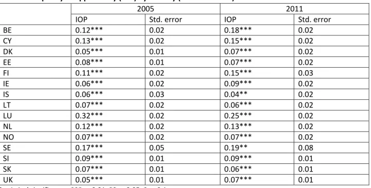
We first present the impact of total family background, namely the education, occupation and activity status of parents, and household financial situation, on income inequality. Table 2 shows the relative measures of inequality of opportunity as presented in equation (4). Across the sample of countries, the results indicate that the extent of inequality of opportunity in gross labour-income ranges between 5%-32% in 2005 and 4%-25% in 2011. Taking the most opportunity unequal country

12_{The syntax file describing the process of harmonization of the variables among countries and between the modules} is available from the authors upon request.

(12)

10

in our analysis, i.e. Luxembourg, the results can be interpreted in the following way: about 35% of the variation in labour income across individuals with similar levels of effort are explained by family background related factors. In particular, individuals with more affluent pedigree manage to obtain higher labour income compared to other individuals with similar levels of effort. At the other

extreme, there are Denmark and the United Kingdom, with 5% of the variation in gross labour

income in 2005 was due to family-related circumstances. Table 2. Inequality of opportunity (IOP) by country (2005 and 2011)

2005 2011

IOP Std. error IOP Std. error

BE 0.12*** 0.02 0.18*** 0.02 CY 0.13*** 0.02 0.15*** 0.02 DK 0.05*** 0.01 0.07*** 0.02 EE 0.08*** 0.01 0.07*** 0.02 FI 0.11*** 0.02 0.15*** 0.03 IE 0.06*** 0.02 0.09*** 0.02 IS 0.06*** 0.03 0.04** 0.02 LT 0.07*** 0.02 0.06*** 0.02 LU 0.32*** 0.02 0.25*** 0.02 NL 0.12*** 0.02 0.13*** 0.02 NO 0.07*** 0.02 0.07*** 0.02 SE 0.17*** 0.05 0.19** 0.08 SI 0.09*** 0.01 0.09*** 0.01 SK 0.07*** 0.01 0.06*** 0.01 UK 0.05*** 0.01 0.07*** 0.01 Statistical significance: *** p<0.01, ** p<0.05, * p<0.1.

Legend: BE- Belgium; CY- Cyprus; DK- Denmark; EE- Estonia; FI- Finland; IE- Ireland; IS- Iceland; LT- Lithuania; LU – Luxemburg; NL- the Netherlands; NO-Norway; SE – Sweden; SI- Slovenia; SK- Slovakia; UK- the United Kingdom. When comparing the results obtained for 2005 and 2011 (Table 2), it is clear that the ranking of countries remains almost intact. This conclusion seems to correspond with the one presented by

Andreoli and Fusco (2017) pointing to no significant changes in the extent of inequality of

opportunity between 2005 and 2011. The countries that showed the highest increase were: Belgium (0.06) and Finland (0.04). In addition, Luxembourg displayed the greatest decline in the extent of inequality of opportunity (0.07). In the case of two countries, i.e. Norway and Slovenia, no change was reported. It should be, however, borne in mind that the results in 2011 could have been affected by the 2008 financial crisis and its aftermath. They caused many countries to implement countercyclical policies followed, at least in some EU member states, by the sizeable austerity measures.

Our results correspond weakly with those reported in other cross-country EU-SILC-based studies, namely, Checchi et al. (2010) and Andreoli and Fusco (2017). With respect to the former, we report similar positions for Denmark, Norway, Slovakia and Slovenia in terms of the relationship between overall income inequality and inequality of opportunity. In line with the latter we show Luxembourg as the most opportunity unequal country. The source of differences may lie in the methodological assumptions since our analysis does not include women, part-time workers, the unemployed and those fulﬁlling domestic tasks and care responsibilities. What is more, we use gross income as the outcome variable, whereas Checchi et al. (2010) use net income. Since country-specific policies play an important role in determining net income, the difference in the outcome variable is likely to

(13)

11

affect the results. With respect to the other cross-country study using the EU-SILC survey, by Andreoli and Fusco (2017), although we use a similar sample and outcome variable, their model specification is limited to a single circumstance variable (i.e., father’s educational attainment), while our analysis contains a vector of multiple circumstance variables.

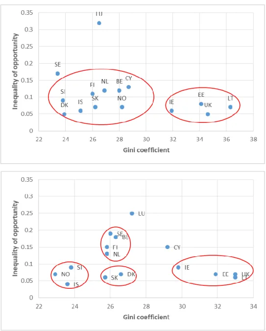
We have also analysed the relation between overall income inequality and the extent of inequality of opportunity by computing pairwise correlations between the two variables. Unlike Perez-Mayo (2019), we do not identify any positive association between overall income inequality, as measured by the Gini coefficient, and the extent of inequality of opportunity. The correlation, as measured by the Pearson coefficient, suggests a rather weak negative relationship (-0.29 for 2005 and -0.12 for 2011). However, one can distinguish groups of countries sharing similar patterns in terms of overall income inequality and inequality of opportunity. As Figure 1 shows, in 2005 we can observe two clusters of countries. The first one comprises more liberal economies such as the United Kingdom, Ireland, Lithuania and Estonia, characterised by relatively high levels of income inequality providing, however, more equitable conditions for employed males to pursue their professional careers. The other group consists of Belgium, Cyprus, Denmark, Iceland, Finland, Slovenia, Slovakia, the Netherlands and Norway, that is, countries with moderate income inequality levels. This group is more heterogeneous in terms of inequality of opportunity than the first group. On the one hand, Scandinavian countries, namely Denmark, Norway and Iceland and eastern European countries, that is Slovenia and Slovakia show rather low levels of inequality of opportunity similar to those characteristic of the first group. On the other hand, Belgium, Cyprus, Finland and the Netherlands display a relatively greater impact of family-related circumstances on individual’s income. The role of Luxembourg and, to some extent, Sweden as outliers needs also to be emphasised. As Andreoli and Fusco (2017) hypothesize, Luxembourg’s position as the most opportunity unequal country might be associated with its specific labour market conditions dominated by the specialized financial sector with the high-skill premium. The results for Sweden might imply a greater role of policies aimed at reducing income inequality through redistribution rather than levelling the field on the labour market. This, however, requires further investigation.

Considering now 2011, Figure 1 shows greater heterogeneity in the relationship between overall income inequality and inequality of opportunity as compared to 2005. Belgium, the Netherlands and Finland joined Sweden forming the group of countries with relatively high levels of inequality of opportunity and moderate income inequality. The cluster of more liberal economies, that is the UK, Ireland, Lithuania and Estonia remained intact. However, it started gravitating towards more moderate territories in terms of overall income inequality. In addition, Norway and Denmark switched positions with respect to income inequality giving rise to two separate groups of countries with relatively small impact of family background on income variation, however, with different levels of total income inequality.

Finally, in order to better understand the nature of the impact of family background on overall income inequality, we calculated the Shapley decomposition for the different circumstance variables considered. As Table 3 shows, there is substantial variation across countries and circumstance categories in 2005. The results reveal that in the majority of countries, age accounted for more than half of inequality of opportunity. However, this is not per se a genuine source of inequality but rather a reflection of differences in individual’s career stages. Apart from age, parents’ education played a major role in explaining inequality of opportunity in 2005 in such countries as: Estonia (54.3%), Ireland (22.2%), Lithuania (66.1%), the Netherlands (18.3%), Norway (9.3%) and

(14)

12

Slovakia (52.2%). For the rest of the countries, the main driving force behind inequality of opportunity were the parents’ economic activity and occupation. The role of the household financial situation was of lesser importance.

When comparing the Shapley decompositions between 2005 and 2011 (Tables 3 and 4), the relative importance, or ranking, of the different circumstance groups seems fairly stable over time. It takes place despite the difference in the actual size of each group in each period and, in general, despite the different sample sizes in 2005 and 2011. However, considerable changes in the decomposition structure are seen in some countries as compared to 2005 (e.g. Sweden or Ireland). Most importantly, the Shapley decompositions for both 2005 and 2011 do not provide us with any apparent pattern that would smoothly correspond with the country rankings on inequality of opportunity.

Figure 1. Income inequality and inequality of opportunity in 2005 (top) and 2011 (bottom)

Note: Gini coefficient refers to the equivalised disposable income based on the EU-SILC survey (Eurostat Database- Income and living conditions).

(15)

13 Table 3. Shapley decomposition by country in % (2005)

BE CY DK EE FI IE IS LT LU NL NO SE SI SK UK

Group1 13.2 3.1 11.0 54.3 15.2 22.2 11.9 66.1 11.3 18.3 9.3 3.0 5.1 52.2 17.7

Group 2 19.4 14.4 26.4 22.1 18.0 19.3 50.6 22.7 20.5 16.8 4.8 22.0 41.9 40.5 71.3

Group 3 9.1 6.9 4.5 14.6 2.9 19.3 6.1 8.4 11.5 3.3 5.8 1.3 6.6 6.2 3.4

Group 4 58.3 75.7 58.1 9.0 64.0 39.2 31.4 2.8 56.7 61.6 80.1 73.7 46.3 1.1 7.7

Legend: Group1- father and mother’s education

Group 2 - father and mother’s economic activity and father’s occupation Group 3 - household self-reported level of financial stress

Group 4 - age

Table 4. Shapley decomposition by country in % (2011)

BE CY DK EE FI IE IS LT LU NL NO SE SI SK UK

Group1 16.6 2.0 19.0 38.8 7.9 9.0 6.5 58.6 14.9 6.2 25.7 42.6 23.8 50.7 19.5

Group 2 15.8 8.7 64.8 50.2 15.2 42.9 11.3 23.4 22.7 44.9 22.0 6.9 33.7 34.9 56.0

Group 3 5.3 1.3 1.9 6.1 7.6 1.5 36.6 16.0 12.0 1.2 8.1 2.3 1.1 13.3 2.3

Group 4 62.4 88.1 14.4 5.0 69.3 46.7 45.6 2.0 50.5 47.7 44.1 48.2 41.4 1.0 22.2

(16)

14

The results for the entire sample of countries without including financial stress as an element of family background confirm the outcomes discussed for the models including household financial stress as a covariate, as reported in Table 5.

Table 5. Inequality of opportunity (IOP) by country excluding financial stress from the set of circumstance variables (2005 and 2011)

2005 2011

IOP Std. error IOP Std. error

BE 0.11*** 0.02 0.17*** 0.15 DE 0.08*** 0.01 0.09*** 0.01 FR 0.13*** 0.01 0.13*** 0.01 AT 0.07*** 0.01 0.01*** 0.02 CY 0.11*** 0.02 0.15*** 0.02 DK 0.05*** 0.01 0.07*** 0.02 EE 0.08*** 0.01 0.07*** 0.02 FI 0.10*** 0.02 0.13*** 0.03 IE 0.05*** 0.01 0.1*** 0.02 IS 0.06*** 0.02 0.03** 0.01 LT 0.07*** 0.02 0.05*** 0.02 LU 0.29*** 0.02 0.23*** 0.02 NL 0.11*** 0.02 0.13*** 0.01 NO 0.06*** 0.01 0.07*** 0.02 SE 0.17*** 0.05 0.19*** 0.07 SI 0.09*** 0.02 0.09*** 0.02 SK 0.07*** 0.01 0.05*** 0.01 UK 0.05*** 0.01 0.08*** 0.01 Statistical significance: *** p<0.01, ** p<0.05, * p<0.1.

We now consider the results by degree of urbanization in order to explore whether large(r) cities can indeed act as social elevators more than smaller urban and rural areas. The results in Table 6 reveal that for 7 out of 13 countries under investigation in 2005 were characterized by the greatest extent of inequality of opportunity in larger cities. Out of the 6 remaining countries, Cyprus, Sweden and Norway turned out to have small cities as the most opportunity unequal places. The dominant role of larger cities in terms of inequality of opportunity is also observed for 2011. For countries such as Belgium, Cyprus, Denmark, Finland, Ireland, Norway, Sweden and the UK there was even an increase in the extent of inequality of opportunity for large cities. Overall, thus, there seems to be more evidence for cities, especially larger ones, as places that benefit more individuals with better family background, i.e. those with more educated and affluent parents who grew up in financial stress-free households.

Table 6. Inequality of opportunity (IOP) by degree of urbanization and country (2005 and 2011)

2005 2011

IOP Std. error Sample size IOP Std. error Sample size

BE

Large urban areas 0.15*** 0.03 740 0.22*** 0.03 709

Small urban areas 0.10*** 0.02 694 0.15*** 0.02 684

Rural areas 0.19** 0.08 73 0.20* 0.11 62

(17)

15

2005 2011

IOP Std. error Sample size IOP Std. error Sample size

Rural areas 0.10*** 0.03 541 0.13*** 0.03 463

DK

Large urban areas 0.10*** 0.03 319 0.11** 0.04 276

Small urban areas 0.06** 0.03 334 0.08** 0.03 323

Rural areas 0.03 0.02 354 0.06 0.04 191

EE

Rural areas 0.09*** 0.02 814 0.07*** 0.02 823

FI

Small urban areas 0.08** 0.04 246 0.21** 0.08 89

Rural areas 0.09*** 0.02 778 0.1*** 0.03 362

IE

Small urban areas 0.05* 0.03 288 0.13** 0.05 145

Rural areas 0.06 0.03 246 0.07 0.04 171

IS

Large urban areas 0.05 0.03 296 0.03* 0.02 315

Rural areas 0.11** 0.05 213 0.1** 0.04 197

LT

Rural areas 0.04** 0.02 543 0.06*** 0.02 528

LU

Rural areas 0.31*** 0.05 255 0.25*** 0.04 479

NO

Small urban areas 0.11*** 0.05 200 0.11** 0.05 185

Rural areas 0.05* 0.03 372 0.07** 0.03 291

SE

Large urban areas 0.28** 0.11 46 0.44*** 0.15 31

Small urban areas 0.31** 0.12 33 0.38 0.22 18

Rural areas 0.16*** 0.06 195 0.22** 0.09 113

SK

Rural areas 0.02* 0.02 776 0.03** 0.01 850

UK

Small urban areas 0.07 0.05 143 0.06*** 0.02 549

Rural areas 0.05 0.09 38 0.08** 0.03 241

Statistical significance: *** p<0.01, ** p<0.05, * p<0.1.

Looking at the Shapley decomposition in Tables 7 and 8, public intervention ought to be tailor-made in order to effectively address the diverse needs of the countries under investigation. For instance, the UK is an example of a country with a great role of parents’ economic activity and occupation in

(18)

16

explaining inequality of opportunity in large cities (71.7% in 2005 and 62 % in 2011). Conversely, Slovakia exemplifies well a country with parents’ education as the main factor affecting inequality of opportunity in large cities (57.1% in 2005 and 73.6% in 2011). Again, the lack of decomposition stability between 2005 and 2011 for several countries (e.g. Sweden and Iceland) calls for caution to be exercised when comparing the results between 2005 and 2011.

Table 7. Shapley decomposition by degree of urbanization and country in % (2005)

BE CY DK EE FI IE IS LT LU NO SE SK UK

Large urban areas

Group1 14.7 3.3 1.7 67.4 11.4 12.2 6.6 68.2 16.8 13.0 8.1 57.1 19.2 Group 2 27.3 23.1 17.5 13.1 15.0 38.6 30.8 17.1 23.1 3.2 37.3 30.6 71.7 Group 3 8.3 4.0 0.5 16.3 2.9 3.2 3.3 5.5 11.7 5.4 3.5 7.4 2.1 Group 4 49.6 69.6 80.3 3.3 70.8 46.0 59.3 9.2 48.4 78.5 51.2 5.0 7.0

Small urban areas

Group1 11.3 9.5 18.3 - 7.1 3.3 - - 9.1 8.8 9.6 46.8 43.8 Group 2 8.6 11.7 20.2 - 17.0 36.6 - - 24.2 7.5 14.2 41.4 28.6 Group 3 10.6 20.2 0.8 - 4.3 45.7 - - 4.6 8.1 23.3 8.6 16.9 Group 4 69.5 58.6 60.7 - 71.7 14.3 - - 62.1 75.5 52.9 3.2 10.8

Rural urban areas

Legend: Same as in Table 3.

Table 8. Shapley decomposition by degree of urbanization and country in % (2011)

BE CY DK EE FI IE IS LT LU NO SE SK UK

Large urban areas

Small urban areas

Group1 13.3 10.7 40.0 - 9.8 28.7 - - 13.2 57.7 34.0 34.2 23.8 Group 2 7.4 8.3 22.0 - 3.0 30.3 - - 22.5 6.6 20.6 26.5 46.0 Group 3 8.4 2.5 2.2 - 0.4 16.9 - - 7.1 1.0 40.1 35.8 7.0 Group 4 70.9 78.5 35.9 - 86.7 24.1 - - 57.2 34.7 5.4 3.5 23.3 Rural areas Group1 21.4 3.3 9.4 29.8 2.8 15.1 11.2 50.7 8.1 29.1 30.7 33.8 5.3 Group 2 57.7 12.3 72.6 54.9 19.5 22.8 8.8 30.0 11.3 9.4 15.9 49.5 45.5 Group 3 11.2 1.4 2.9 4.2 12.0 6.0 63.8 18.6 12.0 1.0 0.2 12.4 1.3 Group 4 9.8 83.1 15.2 11.1 65.7 56.1 16.2 0.7 68.5 60.5 53.2 4.4 48.0

(19)

17

5. Conclusion

This paper contributes to ongoing research on inequality of opportunity in two ways. Firstly, it considers the role of a range of family-related circumstances – i.e., education, occupation and activity status of parents, and household financial situation - and analyses their impact on labour income inequality across 18 European countries and two periods (i.e. 2005 and 2011). Secondly, the paper is the first study to analyse the extent of inequality of opportunity as an explanatory factor of overall income inequality by degree of urbanization with the aim of testing whether cities can indeed function as social elevators.

The findings from the regression analyses show substantial variation in the extent of inequality of opportunity among the countries under investigation. At the one extreme, there is Luxemburg where around 25% of total income inequality was related to family background in 2011. At the other

extreme, there is Iceland where 4%of the variation in gross labour income was due to family-related

environment beyond individual’s control. In addition, several country groups sharing similar patterns in terms of overall income inequality and inequality of opportunity were identified. The distinction between more liberal economies and the rest of the countries is seen with the former being more income unequal, however, with the smaller impact of family-related factors on individual’s income.

In addition, the Shapley decomposition indicated there is considerable variation across countries in terms of the relative importance of specific circumstance variables in explaining inequality of opportunity. In the majority of countries, however, parents’ economic activity and occupation are the main driving force behind inequality of opportunity, followed by parents’ education.

The results by degree of urbanization provide more evidence for cities, especially larger ones, as places that benefit those with more educated and affluent parents who grew up in financial stress-free households. Put differently, cities seem to be more likely to perpetuate, or even strengthen, the competition environment in which individual’s efforts are not the only driver of the professional position and, consequently, labour income. It, thus, undermines their role as social elevators calling for more effective policies to level the field.

(20)

18 References

1. Andreoli F, Fusco A (2017) The evolution of inequality of opportunity across Europe: EU‑SILC evidence. In: Atkinson AB, Guio AC, Marlier E (eds) Monitoring social inclusion in Europe -2017 edition. Eurostat. Publications Office of the European Union, Luxembourg

2. Arneson R (1989) Equality of Opportunity for Welfare. Philosophical Studies 56: 77-93 3. Belhaj-Hassine N (2012) Inequality of Opportunity in Egypt. World Bank Economic Review 26

(2): 265-295

4. Bourguignon F, Ferreira FHG, Menendez M (2007) Inequality of Opportunity in Brazil. Review of Income Wealth, 53(4), 585-618

5. Brunori P (2016) How to Measure Inequality of Opportunity: A Hands-On Guide. Life Course Centre Working Paper Serie no. 2016-04. Dipartimento di Scienze Economiche e Metodi Matematici, University of Bari

6. Brunori P, Ferreira FHG, Peragine V (2013) Inequality of opportunity, income inequality and mobility: some international comparisons. In: Paus E (ed) Getting Development Right: Structural Transformation, Inclusion and Sustainability in the Post-Crisis Era. Palgrave Macmillan

7. Checchi D, Peragine V (2010) Inequality of Opportunity in Italy. Journal of Economic Inequality 8 (4), 429-450

8. Checchi D, Peragine V, Serlenga L (2010) Fair and Unfair Income Inequalities in Europe. IZA DP No. 5025

9. Cogneau D, Mesple-Somps S (2008) Inequality of Opportunity for Income in Five Countries of Africa. DIAL Document de travail DT/2008-04

10. Cohen GA (1989) On the currency of egalitarian justice. Ethics 99: 906-944

11. Corak M (2013) Income Inequality, Equality of Opportunity, and Intergenerational Mobility. Journal of Economic Perspectives 27(3): 79–102

12. Cowell FA (1995) Measuring inequality (2nd_{ed.). Hemel Hempstead: Prentice Hall/Harvester}

Wheatsheaf

13. Dworkin R (1981) What is equality? Part1: Equality of welfare. Part2: Equality of resources. Philos Public Aﬀairs 10, 185- 246, 283-345

14. Ferreira FHG, Gignoux, J (2011) The measurement of inequality of opportunity: theory and an application to Latin America. Review of Income and Wealth, 57(4), 622-657

15. Ferreira FHG, Gignoux J, Meltem A (2011) Measuring Inequality of Opportunity with Imperfect Data: The case of Turkey. Journal of Economic Inequality 9 (4): 651-680

16. Fleurbaey M (2008) Fairness, responsibility and welfare(1st_{ed.). Oxford University Press,} Oxford

17. Juárez FWC, Soloaga I. (2014) Iop: Estimating ex-ante inequality of opportunity Stata Journal 12/2014; 14(4):830-846

18. Kranich L (1996) Equitable Opportunities: An Axiomatic Approach. Journal of Economic Theory 71: 131-147

19. Peragine V (2004) Measuring and implementing equality of opportunity for income. Social Choice and Welfare 22:187-210

20. Perez-Mayo J (2019) Inequality of opportunity, a matter of space? Regional Science Policy and Practice 11:71-87

(21)

19

21. Piraino P (2012) Inequality of opportunity and intergenerational mobility in South Africa. Paper presented at the 2nd World Bank Conference on Equity. June 27th, 2012, Washington DC

22. Pistolesi N (2009) Inequality of opportunity in the land of opportunities, 1968-2001. Journal of Economic Inequality 7: 411-433

23. Ramos X, Van de Gaer D (2012) Empirical Approaches to Inequality of Opportunity: Principles, Measures, and Evidence. IZA DP No. 6672

24. Rawls J (1971) A Theory of Justice. Oxford University Press, Oxford

25. Roemer J (1993) A pragmatic theory of responsibility for the egalitarian planner. Philosophy and public aﬀairs 22, 146-166

26. Roemer J (1998) Equality of Opportunity. Harvard University Press, Cambridge

27. Salvi A (2007) An empirical approach to the measurement of equality of opportunity. Universit`a degli Studi di Milano

28. Sen A (1985) Commodities and Capabilities. North Holland, Amsterdam

29. Singh A (2011) Inequality of opportunity in earnings and consumption expenditure: The case of Indian men. Review of Income and Wealth 58 (1)

30. Van de Gaer D (1993) Equality of opportunity and investment in human capital. Ph.D. Dissertation, Catholic University of Leuven

31. Van Kerm P, Alperin M (2013) Inequality, growth and mobility: The intertemporal distribution of income in European countries 2003-2007. Economic Modelling, 35, 931-939

(22)

20

Appendix

Table 1. Explanatory variables by country - % of the sample (2005)

AT13 _BE _CY _DE _DK _EE _FI _FR _IE _IS _LT _LU _NL _NO _SE _SI _SK _UK Education (father) not higher 96.11 84.24 93.65 70.54 84.57 85.41 80.87 91.42 91.14 87.61 89.29 87.47 83.01 76.49 86.18 95.40 91.04 84.52 higher 3.89 15.76 6.35 29.46 15.43 14.59 19.13 8.58 8.86 12.39 10.71 12.53 16.99 23.51 13.82 4.60 8.96 15.48 Education (mother) not higher 98.27 89.48 96.28 91.52 87.20 84.25 86.33 94.30 92.92 92.33 89.46 92.07 93.78 74.84 89.85 98.08 95.66 88.84 higher 1.73 10.52 3.72 8.48 12.80 15.75 13.67 5.70 7.08 7.67 10.54 7.93 6.22 25.16 10.15 1.92 4.34 11.16

Activity status (father)

Employed & self-employed (inc. family workers) 97.04 91.50 99.05 96.79 93.62 98.83 92.68 97.95 96.64 99.82 98.12 98.39 95.43 98.67 97.97 97.19 97.40 97.85 unemployed 0.45 0.47 0.06 0.56 1.26 0.08 0.06 0.31 1.63 - 0.09 0.12 0.61 0.07 0.51 0.23 0.24 1.59 retirement 1.71 0.76 0.06 1.65 - 0.39 5.07 0.50 0.31 - 0.51 1.24 0.56 1.25 1.10 1.36 1.56 0.43 Domestic tasks and other 0.80 7.27 0.84 1.00 5.12 0.70 2.19 1.24 1.43 0.18 1.28 0.25 3.40 - 0.42 1.21 0.80 0.13

Activity status (mother)

Employed & self-employed (inc. family workers) 43.88 36.04 37.74 46.62 64.88 93.98 85.26 51.41 27.07 58.28 86.11 36.19 26.01 97.88 66.75 67.40 80.65 58.09 unemployed 0.14 0.98 0.05 0.44 1.88 - - 0.15 0.20 - 0.08 0.06 0.05 0.07 0.08 0.83 0.86 1.21 retirement 0.39 0.58 - 0.69 26.90 0.13 2.54 0.06 - 0.33 0.15 0.24 - 0.66 0.57 0.96 1.17 0.09 Domestic tasks and other 55.59 62.41 62.21 52.25 6.34 5.89 12.20 48.39 72.73 41.39 13.66 63.50 73.93 1.39 32.59 30.81 17.33 40.61

Household self-reported level of financial stress

Very bad - 4.05 7.37 - 3.23 5.49 7.23 - 6.92 2.55 10.94 6.63 4.19 2.84 3.50 15.32 3.84 10.19 bad - 5.01 16.92 - 4.50 15.16 10.32 - 10.09 4.30 21.81 9.95 8.43 3.60 7.24 24.00 15.56 11.13 fair - 11.81 41.22 - 14.76 38.93 25.33 - 22.16 15.13 28.38 20.33 16.08 13.22 13.17 32.22 32.41 21.21 good - 11.30 27.82 - 18.20 21.65 21.03 - 21.96 15.13 16.98 16.04 18.39 28.44 20.73 15.32 27.12 21.62 Very good - 67.83 6.67 - 59.31 18.78 36.09 - 38.87 62.90 21.89 47.04 52.92 51.90 55.37 13.15 21.08 35.86

Main occupation (father)

Managers 6.20 10.75 1.28 7.12 11.21 11.72 11.70 11.24 26.25 19.13 7.09 9.87 20.75 13.46 9.90 4.75 6.84 5.77 Professional 3.12 10.24 4.18 13.38 11.21 6.85 8.39 8.95 9.48 10.02 8.38 8.00 9.65 9.25 7.26 5.29 6.36 6.67 Technicians and associate professionals 10.45 6.57 4.96 10.82 8.77 6.22 12.69 8.36 2.71 9.11 3.50 14.37 14.05 17.29 8.25 9.66 10.53 8.65 Clerical support workers 5.99 11.13 4.18 8.03 4.67 1.26 1.92 5.76 6.46 0.91 2.14 6.12 6.39 3.53 5.94 3.75 3.25 20.36 Service and sales workers 9.27 5.56 11.75 2.97 5.39 1.34 3.24 3.19 6.56 6.19 2.48 2.81 4.64 4.74 6.60 4.98 3.54 24.74 Skilled agricultural, forestry and fish 14.39 4.17 21.45 6.76 12.37 3.23 21.35 12.02 0.73 21.13 6.67 8.62 2.47 10.68 9.57 15.63 3.64 0.84 Craft and related trades workers 26.93 23.89 23.79 31.61 19.05 28.48 21.15 24.01 18.54 20.95 26.24 23.80 22.26 23.91 33.00 26.82 29.13 2.10 Plant and machine operators, and assemblers 7.53 9.99 9.36 12.10 8.48 28.95 13.48 17.88 10.21 8.01 20.51 22.05 11.58 15.86 16.50 22.38 20.24 9.85 Elementary occupations 15.31 9.86 18.22 6.13 13.59 11.25 3.77 7.33 17.60 4.37 21.71 4.12 4.52 1.28 1.32 5.52 15.63 20.78 Not paid domestic activities 0.82 7.84 0.84 1.07 5.25 0.71 2.31 1.25 1.46 0.18 1.28 0.25 3.68 - 1.65 1.23 0.83 0.24

Urbanization

Large urban areas 27.53 49.10 55.40 41.86 30.90 32.72 25.55 45.24 40.39 58.67 51.99 46.72 - 51.03 17.92 - 26.18 75.61 Small urban areas 27.88 45.83 13.33 39.93 31.76 - 16.20 38.46 31.32 - - 34.02 - 17.60 13.99 - 35.96 19.83 Rural areas 44.59 5.06 31.27 18.21 37.34 67.28 58.25 16.29 28.28 41.33 48.01 19.27 - 31.37 68.09 - 37.86 4.56

Total number of observations 2532 1896 2085 4893 3152 1834 4216 3658 1941 1667 1458 1858 4116 3255 2745 4575 2525 3708

13_{AT- Austria; BE- Belgium; CY- Cyprus; DE- Germany; DK- Denmark; EE- Estonia; FI- Finland; FR- France; IE- Ireland; IS- Iceland; LT- Lithuania; LU –Luxemburg; NL- the Netherlands;} NO-Norway; SE – Sweden; SI- Slovenia; SK- Slovakia; UK- the United Kingdom.

(23)

21

Table 2. Explanatory variables by country - % of the sample (2011)

AT BE CY DE DK EE FI FR IE IS LT LU NL NO SE SI SK UK Education (father) not higher 85.55 78.04 92.20 71.40 78.35 81.15 76.58 88.55 83.17 85.04 90.37 87.79 79.00 69.98 81.61 90.45 90.30 83.25 higher 14.45 21.96 7.80 28.60 21.65 18.85 23.42 11.45 16.83 14.96 9.63 12.21 21.00 30.02 18.39 9.55 9.70 16.75 Education (mother) not higher 95.60 83.79 95.16 89.46 80.60 77.93 81.37 90.67 86.85 93.33 88.17 91.82 91.08 78.09 79.38 93.17 94.90 85.93 higher 4.40 16.21 4.84 10.54 19.40 22.07 18.63 9.33 13.15 6.67 11.83 8.18 8.92 21.91 20.62 6.83 5.10 14.07

Activity status (father)

Employed & self-employed (inc. family workers) 98.19 97.09 98.64 97.56 98.84 98.05 95.40 97.31 96.09 98.78 98.85 98.13 97.72 98.45 97.88 95.38 99.25 95.89

unemployed 0.10 0.51 0.19 0.67 0.46 0.07 2.72 0.42 2.28 0.17 - 0.26 0.33 0.27 0.37 1.22 0.13 1.90

retirement 1.21 0.85 0.80 1.34 0.58 0.65 0.94 0.54 0.65 - 0.35 0.85 0.11 1.28 1.47 2.31 0.22 1.00

Domestic tasks and other 0.50 1.54 0.37 0.43 0.12 1.23 0.94 1.73 0.98 1.05 0.80 0.77 1.83 - 0.28 1.09 0.40 1.21 Activity status (mother)

Employed & self-employed (inc. family workers) 53.09 48.53 45.47 53.39 72.53 93.20 90.79 56.12 35.57 71.40 88.63 41.75 34.20 74.82 79.35 72.42 89.66 65.06

unemployed 0.10 0.72 0.06 0.78 0.32 0.06 3.04 0.16 0.94 - 0.33 0.04 0.27 0.63 0.36 0.84 0.30 8.58

retirement 0.34 0.22 - 0.44 0.85 0.32 1.01 0.16 - - - 0.45 - 1.16 0.90 0.97 0.17 0.47

Domestic tasks and other 46.47 50.53 54.47 45.39 26.30 6.42 5.16 43.55 63.49 28.60 11.04 57.76 65.53 23.39 19.39 25.76 9.87 25.89 Household self-reported level of financial stress

Very bad 7.06 2.41 10.79 2.93 1.45 0.70 1.36 3.42 2.95 2.07 1.60 3.42 1.22 0.98 2.30 6.81 2.43 2.98

bad 9.47 5.68 11.89 8.31 4.66 4.88 5.81 7.76 7.45 7.06 8.16 8.15 3.83 3.56 5.79 13.62 5.57 6.47

fair 56.37 41.85 48.64 54.18 47.10 72.94 65.06 60.83 51.86 62.99 62.32 51.63 38.24 46.75 39.58 65.30 59.81 59.89 good 21.24 41.64 23.77 27.69 34.68 19.65 24.46 24.21 29.81 21.51 26.40 30.89 48.67 41.05 39.58 11.05 28.29 25.27

Very good 5.86 8.41 4.91 6.90 12.11 1.84 3.30 3.78 7.92 6.37 1.52 5.91 8.03 7.66 12.76 3.21 3.89 5.39

Main occupation (father)

Armed Forces Occupations 0.77 - 0.63 - - 0.92 1.15 1.31 1.85 - 0.74 0.95 1.59 2.03 1.46 0.92 1.03 1.66 Managers 3.75 6.99 1.38 5.64 11.74 8.97 5.49 8.91 16.13 13.38 6.09 6.64 9.23 13.57 6.34 1.98 4.86 11.26 Professional 5.80 15.12 6.76 11.69 13.68 8.35 14.43 7.31 12.94 12.32 8.86 9.59 12.41 12.65 15.61 6.50 7.06 16.51 Technicians and associate professionals 8.26 13.80 8.89 17.66 8.60 5.75 12.39 13.10 5.88 7.39 3.87 13.54 18.22 16.90 8.29 14.34 10.93 9.22 Clerical support workers 6.21 11.09 2.57 6.44 5.08 1.53 2.30 8.32 3.19 2.46 1.85 5.86 7.06 3.60 2.93 4.73 3.41 4.64 Service and sales workers 15.29 6.05 11.14 6.46 11.50 1.92 5.62 3.93 9.92 9.51 2.49 3.38 7.23 4.52 9.27 6.43 4.53 7.18 Skilled agricultural, forestry and fish 13.08 4.41 15.33 5.20 12.95 5.29 14.30 9.84 14.29 19.54 7.66 9.11 7.92 9.14 10.73 7.77 2.38 3.26 Craft and related trades workers 31.45 22.37 27.41 28.21 28.93 25.13 19.80 15.83 15.46 22.18 25.00 26.20 22.78 22.44 29.76 28.95 31.73 24.74 Plant and machine operators, and assemblers 6.93 14.62 11.76 14.63 6.05 33.41 19.03 5.70 7.23 8.45 18.27 19.96 9.00 11.45 12.20 10.24 22.48 12.09 Elementary occupations 7.95 3.84 13.77 3.62 1.33 7.43 4.21 23.98 12.10 3.70 24.35 3.99 2.68 3.69 1.95 17.02 11.17 8.17 Not paid domestic activities 0.51 1.70 0.38 0.47 0.12 1.30 1.28 1.78 1.01 1.06 0.83 0.78 1.88 - 1.46 1.13 0.42 1.27

Urbanization

Large urban areas 29.53 49.36 53.81 45.55 31.29 32.44 25.10 42.03 39.57 61.55 50.74 43.93 - 55.15 18.60 - 26.86 53.31

Small urban areas 29.73 45.39 16.13 38.73 43.37 - 14.59 38.91 27.57 - - 34.60 - 17.47 16.18 - 32.41 32.04

Rural areas 40.74 5.25 30.06 15.72 25.34 67.56 60.32 19.06 32.86 38.45 49.26 21.47 - 27.38 65.22 - 40.73 14.65 Total number of observations 2489 2040 1903 5164 2474 1902 3339 4035 1059 1571 1482 2627 4206 2370 2936 4767 2703 2840