* Corresponding author: E-mail: [email protected]
Received: June 28, 2017 Approved: November 5, 2017
How to cite: Machado IR, Giasson E, Campos AR, Costa JJF, Silva EB, Bonfatti BR. Spatial disaggregation of multi-component soil map units using legacy data and a tree-based algorithm in Southern Brazil. Rev Bras Cienc Solo. 2018;42:e0170193.
https://doi.org/10.1590/18069657rbcs20170193
Copyright: This is an open-access article distributed under the terms of the Creative Commons Attribution License, which permits unrestricted use, distribution, and reproduction in any medium, provided that the original author and source are credited.
Spatial Disaggregation of
Multi-Component Soil Map Units
Using Legacy Data and a Tree-Based
Algorithm in Southern Brazil
Israel Rosa Machado(1)
, Elvio Giasson(2)
, Alcinei Ribeiro Campos(1)*
, José Janderson Ferreira Costa(1)
, Elisângela Benedet da Silva(3)
and Benito Roberto Bonfatti(4)
(1)
Universidade Federal do Rio Grande do Sul, Programa de Pós-Graduação em Ciência do Solo, Porto Alegre, Rio Grande do Sul, Brasil.
(2)
Universidade Federal do Rio Grande do Sul, Departamento de Solos, Porto Alegre, Rio Grande do Sul, Brasil. (3)
Empresa de Pesquisa Agropecuária e Extensão Rural de Santa Catarina - Centro de Informações de Recursos Ambientais e de Hidrometeorologia de Santa Catarina, Florianópolis, Santa Catarina, Brasil. (4)
Universidade do Estado de Santa Catarina, Centro de Ciências Agroveterinárias, Departamento de Engenharia Ambiental e Sanitária, Lages, Santa Catarina, Brasil.
ABSTRACT: Soil surveys often contain multi-component map units comprising two or more soil classes, whose spatial distribution within the map unit is not represented. Digital Soil Mapping tools supported by information from soil surveys make it possible to predict where these classes are located. The aim of this study was to develop a methodology to increase the detail of conventional soil maps by means of spatial disaggregation of multi-component map units and to predict the spatial location of the derived soil classes. Three digital maps of terrain variables - slope, landforms, and topographic wetness index - were correlated with the soil map and 72 georeferenced profiles from the Porto Alegre soil survey. Explicit rules that expressed regional soil-landscape relationships were formulated based on the resulting combinations. These rules were used to select typical areas of occurrence of each soil class and to train a decision tree model to predict the occurrence of individualized soil classes. Validation of the soil map predictions was conducted by comparison with available soil profiles. The soil map produced showed high agreement (80.5 % accuracy) with the soil classes observed in the soil profiles; Ultisols and Lithic Udorthents were predicted with greater accuracy. The soil variables selected in this study were suitable to represent the soil-landscape relationships, suggesting potential use in future studies. This approach developed a more detailed soil map relevant to current demands for soil information and has potential to be replicated in other areas in which data availability is similar.
INTRODUCTION
The important role of soils in maintaining life on Earth dictates they should be used in a sustainable way and highlights the need for pedological information, such as soil properties and spatial distribution. The most common source of this information is the soil survey, which generally comprises a soil map accompanied by a descriptive report with a dataset of independent pedons.
However, Brazilian soil surveys that cover the entire country only exist at the reconnaissance level, containing soil maps with small scales (less than 1:750,000), and more detailed maps are rarely available (Giasson et al., 2006). Because of the small scale of these maps and/or complex arrangement of soils in the landscape, in most cases a map unit (MU) aggregates more than one soil component, forming a multi-component MU. Thus, there is no graphical representation of the distribution of these components in the soil map in these multi-component MU, and the only information contained in the survey report describes their general spatial distribution in the landscape and/or the percentage of each component within the MU. With these characteristics, they may not meet current demands for soil information, e.g., the valuation of ecosystem services provided by soils or the delineation of wetlands (Vincent et al., 2018).
However, existing soil surveys can be an important starting point for generating more detailed soil maps. One possibility to refine information on soil distribution is to use spatial disaggregation of multi-component MUs. Spatial disaggregation follows Digital Soil Mapping (DSM) techniques and environmental covariates to separate soil components within a multi-component MU, based on spatial relationships or patterns between soils and the landscape (Sarmento et al., 2017; Vincent et al., 2018). The objective is to use a map with fewer details to produce an enhanced map that represents the distribution of the soil components, i.e., a map with more single MUs (Nauman et al., 2014). Spatial disaggregation of the multi-component MUs takes advantage of valuable sources of information, such as legacy data, which can be observational points (independent pedons) and/or soil maps with their respective descriptive reports.
Tree-based models have been widely used in soil class prediction with DSM, due to ease of understanding and discussion, the ability to process large datasets, and robustness as a predictive technique (ten Caten et al., 2012; Bagatini et al., 2016). Following the same logic of conventional soil mapping, in which pedologists seek to establish conceptual relationships between soils and environmental parameters, DSM tree-based models can be used to correlate soil components or properties with environmental covariates, e.g., elevation and slope, to produce more detailed maps. These algorithms have been used for the disaggregation of multi-component MUs of conventional soil maps (Häring et al., 2012; Nauman et al., 2014; Nauman and Thompson, 2014; Sarmento et al., 2017; Vincent et al., 2018) or geological studies (Bui and Moran, 2001) and to describe the spatial variation of soil properties, such as organic carbon, with more detail (Kerry et al., 2012).
We aimed to present a methodology to increase the detail of a soil map by disaggregating the multi-component MUs of the soil map of the municipality of Porto Alegre using available soil information and tree models to generate an enhanced soil map. This approach based on available legacy data allows substantial reduction in the number and extent of field trips, which are a considerable part of the cost of a soil survey.
MATERIALS AND METHODS
Study area
hills. At lower levels, there are more recent formations, such as eluvial deposits of granites and gneisses and partially reworked colluvial and alluvial deposits, the latter forming terraces and sand barriers. Along the streams and on the islands in the Jacuí River delta, deposits of sediments of fluvial origin occur. On the banks of Guaíba Lake, more recent lagoon and marine sediment deposits form sand coastal plains (Philipp, 2008). The elevation ranges from 0.1 m (Jacuí River delta) to 311 m (Santana Hill) (Penter et al., 2008; Hasenack et al., 2010).
The region is in a transition between two major Brazilian biomes, the Pampas and the Atlantic Forest; the vegetation comprises a mosaic of wood- and grasslands, as well as various pioneer formations (Hasenack et al., 2008). The climate, according to Köppen system, is Subtropical Humid (Cfa), with an annual mean temperature of 19.5 °C and annual mean rainfall of 1,320 mm, well distributed throughout the year (Inmet, 2016).
The most common soils classes according to Soil Taxonomy (Soil Survey Staff, 2014) and Brazilian Soil Classification System (Santos et al., 2013) are Ultisols (Argissolo Vermelho Distrófico), Inceptisols (Cambissolo Háplico Alítico), and Lithic Udorthents (Neossolo Litólico Distrófico), usually found at higher elevations, whereas Albaquults (Planossolo Háplico Distrófico), Plintaquults (Plintossolo Argilúvico Distrófico), and Aquents (Gleissolo Háplico Alítico) occur in low-lying areas (Schneider et al., 2008).
Available soil and terrain database
The Porto Alegre soil survey (Schneider et al., 2008), part of a comprehensive environmental assessment (Hasenack et al., 2008), covers the entire municipality and contains a soil map published at 1:50,000 scale. It is formed by twelve MUs: one single MU, one MU composed of terrain types, and ten multi-component MUs. Of these last MUs, nine are soil associations and one is an undifferentiated group.
The original 72-pedon dataset was obtained from the pedologists who carried out the original soil survey, and it was used as an information source in addition to the soil map. Pedon data included soil classification to the second categorical level of the Brazilian Soil Classification System (SiBCS), the geographical coordinates, slope, and landscape position of each pedon. A digital hypsometric map (line vector format with 1 m interval contours), from Hasenack et al. (2010), was used to produce a digital elevation model (DEM) with a 15-m pixel resolution with ArcMap™ 10.2 (ESRI, 2013).
Assignment of soil-landscape relationships and creation of training area
This methodology follows a rationale similar to that of Nauman et al. (2014), Nauman and Thompson (2014), and Sarmento et al. (2017) (Figure 2). The initial effort was to select areas typifying the occurrence of each soil component, where there is high probability that a certain soil component will occur. Through selection of these areas, it was possible to correlate the environmental variables with the soil components and, using prediction models, to generate maps with MUs containing only single components.
The multi-component MUs used for disaggregation were CX, GX, PV1, PV2, and SG1 (Table 1), which occupy approximately 80 % of the municipal area. These MUs were chosen because the soil components that compose them occur in distinguishable positions in the landscape, as described in the survey report, thus enabling the individualization of each soil component to generate a map with the largest number of simple MUs. The areas of the MUs not used in the disaggregation were maintained within their original limits.
the slope and the landscape position of each pedon. LandMapR produces landscape segmentation (into 15 landforms) based on elevation, surface contours, slope length, relative slope position, and other variables (MacMillan et al., 2000; MacMillan et al., 2005; Sarmento et al., 2017). The relation between LandMapR and the landforms and the landscape position of each soil component was established by comparing the description of each landform provided by MacMillan (2003) and the description of the position occupied by each soil component in the landscape, which is contained in the soil survey report (Schneider et al., 2008).
After that, the pedons were cross-tabulated with the slope and landform maps and the soil map containing the delimitations of the MUs to generate a table with the combination of these three variables. Analyzing the combinations, we noted that the slope variable did not contribute to explain the occurrence of soil components commonly found at lower elevations, which have poorly drained soils, such as Aquents, Albaquults, and Plintaquults. Therefore, it was necessary to include an additional environmental variable, the Topographic Wetness Index (TWI). This index, developed by Beven and Kirkby (1979), combines the upslope contributing area and slope to explicitly quantify topographic control over hydrological processes (Sørensen and Seibert, 2007). The index was generated in ArcMap. A cross- tabulation of poorly drained soil pedons and TWI was conducted and showed high correlation between these soils and this variable. Earlier studies by Giasson et al. (2006) and Nauman et al. (2014) also used the TWI to differentiate areas with contrasting drainage in DSM studies. Subsequently, the study was conducted separately in two subareas: MUs containing well-drained soils (WDS) and imperfectly/poor drained soils (IPDS).
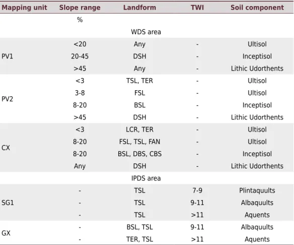
The most common combinations between MU, slope, and landform were selected for the WDS areas, and the most common combinations between MU, TWI, and landform were selected for the IPDS areas. From these combinations, rules that explain the occurrence of soil components were created. For example: Inceptisols are expected to occur on a Divergent Backslope (DBS) landform with slopes ranging from 23-30 % in the multi-component MU CX. Aquents are expected to occur in a Toe Slope (TSL) landform with TWI ranging from 10 to 15 in the multi-component MU GX. For each soil component, not only one, but several individual rules were created. At the end of the rule creation process for a total of six different individualized soil components, a total of 210 unique soil occurrence rules were created (Table 2).
URUGUAY URUGUAY
ARGENTINA
N
BRAZIL
ARGENTINA
Rio Grande do Sul
Santa Catarina
0 50 100 200 300 km
57° W 55° W 53° W 51° W
33°
S3
1°
S2
9°
S2
7° S
Figure 2. Schema of methodological steps for disaggregating soil map units in the Porto Alegre municipality area.
First notion about soil information SOIL
SURVEY REPORT
Crosstabulation
Table with the environmental properties of each pedon
Split the area in WDS and IPDS areas
Creation of
soil-landscape rules
Selection of typical areas of each soil component
Sampling
Crosstabulation with the sample points
Tree-based model training
Non-disaggregated areas
Merge
Final map
Accuracy assessment VISUAL ANALYSIS
These rules were translated into logical expressions for insertion into the ArcMap’s Raster Calculator tool. Areas corresponding to the rule combinations of landform, MU, and slope (for the WDS areas) or landform, MU, and TWI (for the IPDS areas) were selected, aiming to represent the typical areas for each soil component (Figure 2). After selection, these typical areas were converted to polygon vector format to facilitate the creation of sample points that were needed for the predictive model. Sample points were created in ArcMap™ 10.2 with the Sampling Design Tool (Buja and Menza, 2013). We used a stratified random sampling approach in which a given point density was defined and applied to all polygons, resulting in similar density for all the polygons of the training area. This approach allowed better distribution of points across polygons, as opposed to random sampling, which tends to provide greater density of points in large polygons, thus reducing the importance of the information contained in small polygons (Odgers et al., 2014). The point density chosen was approximately 2.5 points per hectare, as suggested by Sarmento et al. (2012) and Bagatini et al. (2015) for sampling density in DSM. The sampling process resulted in selection of approximately 50,000 sampling points in the WDS area and approximately 38,000 sampling points in the IPDS area for use in the predictive model.
Table 1. Soil map units in the Soil Survey map of Porto Alegre, RS, Brazil (adapted from Schneider et al., 2008)
Map unit
Drainage(1) Soil Taxonomy Brazilian System
Area
ID Type Principal Inclusions Principal Inclusions
%
PV1 Undifferentiated Group WDS Ultisols
Inceptisols Argissolos Cambissolos 6.9 Lithic Udorthents Neossolo litólico
PV2 Association WDS Ultisols and Inceptisols Lithic Udorthents
Argissolos and Cambissolos
Neossolo
litólico 15.8
CX Association WDS Inceptisols and Lithic
Udorthents Ultisols Cambissolos and Neossolo Litólico Argissolos 14 Rocky outcrops Afloramentos rochosos
SG1 Association IPDS Albaquults, Aquents,
and Plintaquults
-Planossolo Háplico, Gleissolo Háplico, and
Plintossolo Argilúvico - 26.8
SG2 Association NU Albaquults, Aquents,
and Fluvents
-Planossolo Háplico, Gleissolo Háplico,
and Neossolo Flúvico - 1.9
GX Association IPDS Aquents and
Albaquults
-Gleissolo Háplico
and Planossolo
Hidromórfico - 14.6
G1 Association NU Aquents and Fluvents Histosols Gleissolo Háplico and Neossolo Flúvico Organossolos 7.4
G2 Association NU Aquents and Albaquults
and Terrain Types(2) Plintaquults
Gleissolo Háplico, Planossolos, and
Tipos de Terreno(2)
Plintossolo
Argilúvico 6.3
RQ Association NU Quartzipsamments
and Aquents
-Neossolo
Quartzarênico and
Gleissolo Háplico - 2.5
RU1 Simple NU Fluvents Aquents Neossolo Flúvico Gleissolo Háplico 0.1
RU2 Association NU Fluvents and Terrain
Types Aquents
Neossolo Flúvico and
Tipos de Terreno
Gleissolo
Háplico 2.1
TT Terrain Type NU - - Tipos de Terreno - 1.6
(1)
Drainage classes created in this study. WDS = well-drained soil area; IPDS = imperfectly/poorly drained soil area; NU = not used for disaggregation; - = no inclusions. (2)
Tree-based model implementation
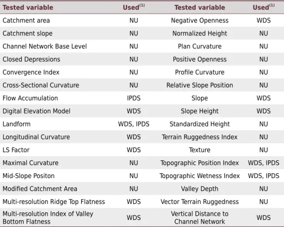
To implement the predictive model, a set of 32 environmental variables (Table 2) was generated in SAGA-GIS (Conrad et al., 2015) from the DEM. These variables were then cross-tabulated in ArcMap with the sampling points from the previous step. In this step, each sampling point received a combination of values from the variables. The process generated two tables, one for the WDS area and one for the IPDS area. These tables were inserted in the data-mining software WEKA 3.6 (Hall et al., 2009) and formed the database for implementation of the predictive models for generation of the disaggregated soil map. With the Attribute Selection function of WEKA, the variables were tested for their contribution to soil component mapping in the predictive model. Based on statistical analysis of the dataset, this tool searched which subset of properties worked best for prediction. Then, relevant properties could be selected, and the redundant or irrelevant ones could be discarded, resulting in a model that was simpler, faster, and easier to interpret (Hall and Holmes, 2003).
The predictive model chosen was the decision tree algorithm J48, which is a Java implementation of the C4.5 algorithm (Quinlan, 1993) in the WEKA data-mining tool. The choice was based on the satisfactory results shown by this algorithm in other DSM studies (Giasson et al., 2011; Costa, 2016). Pruning of the decision tree was established to avoid overfitting of the model; thus, terminal nodes with less than 10 pixels were suppressed. Values of 5, 15, 20, and 30 pixels were tested, but the value of 10 was chosen because it resulted in a predictive model with accuracy higher than 90 % without an excessive, time-consuming number of rules. Model training was performed with 50 % of the points, while the other half was used for validation.
Table 2. Examples of rules created to describe the typical location of soil components within the five mapping units based on the slope ranges, landforms, and Topographic Wetness Index (TWI)
Mapping unit Slope range Landform TWI Soil component
%
WDS area
PV1
<20 Any - Ultisol
20-45 DSH - Inceptisol
>45 Any - Lithic Udorthents
PV2
<3 TSL, TER - Ultisol
3-8 FSL - Ultisol
8-20 BSL - Inceptisol
>45 DSH - Lithic Udorthents
CX
<3 LCR, TER - Ultisol
8-20 FSL, TSL, FAN - Ultisol
8-20 BSL, DBS, CBS - Inceptisol
Any DSH - Lithic Udorthents
IPDS area
SG1
- TSL 7-9 Plintaquults
- TSL 9-11 Albaquults
- TSL >11 Aquents
GX - BSL, TSL 9-11 Albaquults
- TER, TSL >11 Aquents
The resulting tree-based models, one for the WDS area and the other for the IPDS area, were implemented using the Raster Calculator in ArcMap™ 10.2. This step generated two soil maps, one with only the soils of the WDS area and another with only the soils of the IPDS area. These two maps were merged with the areas that were not disaggregated to form one final soil map with approximately 80 % of its area containing individual soil components.
Map accuracy assessment
The accuracies of the original and disaggregated soil maps were assessed by intersecting the maps with the georeferenced pedon dataset (Häring et al., 2012; Nauman et al., 2014; Nauman and Thompson, 2014; Sarmento et al., 2017). A 30-m circular buffer was created in each pedon, similar to that performed by Sarmento et al. (2014), Nauman and Thompson (2014), Heung et al. (2016), and Vincent et al. (2018). This buffer is created for the purpose of disregarding the precision error involved in the GPS equipment used to collect the geographic coordinates of the pedons, which may be more than 20 meters in some cases, depending on the atmospheric conditions and the equipment used. The prediction was computed correctly when any pixel in the buffered area matched that of the reference pedon (Smith et al., 2012; Nauman and Thompson, 2014; Sarmento et al., 2017).
The risk of a biased validation using the soil pedons was deemed low because their spatial location was not used directly as a training area. The pedons were used as an information source about the environmental conditions that each soil component occurs, aiming to create soil-landscape rules for selecting typical areas of each soil component. These selected areas, here called “training areas”, were used for training the tree-based model. The use of these pedons for validation helped attain one of our objectives, namely to reduce costs on field trips in elaborating a soil survey.
RESULTS AND DISCUSSION
A visual comparison between the original map and the disaggregated map provides a first assessment of the improvement obtained from MU disaggregation (Figure 3). Whereas in the original map each MU was composed of more than one soil component, in the disaggregated map, each MU is formed by only one. Unlike the original map in which lines delimit the MUs, the disaggregated map represents the distribution of MUs through pixels, enabling more gradual and continuous transitions between the MUs, as occurs in the landscape. In addition, the pixels may represent the inclusions, unlike the original map of polygons, in which it would not be possible to know their location. Thus, the disaggregated map provides more detailed information on soil components.
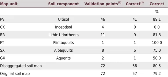
Soil components which had more georeferenced pedons available showed higher performance, similar to that verified by Häring et al. (2012), with 89.1, 81.8, and 75.0 % correct predictions for the MUs (single component) of PV, RR, and SX, respectively. The MU FT exhibited 100 % correct predictions, but the availability of only one pedon imposes only two possible results, 0 or 100 %, making it difficult to evaluate the real value of correct predictions. Aside from this exception, components with low availability of georeferenced points had the worst concordances, at 0 and 50 % for Inceptisols and Aquents, respectively. These results reflect the difficulty of creating soil-landscape rules from a limited amount of information about the environmental conditions in which a given soil component occurs.
In the WDS areas, the disaggregated map showed an extensive area mapped with Ultisols, followed by Lithic Udorthents at the tops and steep slopes of hills (Figure 3). Even in the original MU CX, the Ultisols occupied an extensive area, in contrast with the report of the original soil survey (Table 1), which suggests that Inceptisols and Lithic Udorthents
Figure 3. Comparison of a part of the original (a) and of the disaggregated (b) soil map. The acronyms in the images and in the legend correspond to the map units of the original and of the disaggregated soil map, respectively.
CX
SG1
PV2
SG2
CX
PV1
PV2
PV1
SG1
PV2
CX
PV2
CX
PV2
PV2
PV2
CX
SG1
PV2
SG2
CX
PV1
PV2
PV1
SG1
PV2
CX
PV2
CX
PV2
PV2
PV2
–
PV CX
RR FT
SX1 GX
SX2
MU limits km (a)
(b)
predominate in this MU. However, unlike the original survey, recent studies have shown that Inceptisols tend to occur under very specific topographic conditions, occupying narrow bands between Ultisols and Lithic Udorthents. In a study of the soils of Extrema Hill, in Porto Alegre, Medeiros et al. (2013) described the occurrence of Ultisols in places where the soil-landscape relationship would suggest the presence of Inceptisols, indicating that in the region, these soils occupy narrow zones of transition between Ultisols and Lithic Udorthents. Along the toposequence studied, these authors described the occurrence of three Ultisols, one Lithic Udorthent, and no Inceptisol. In the same municipality, Medeiros (2014) analyzed two toposequences, one in Santana Hill and one in São Pedro Hill, and found four Ultisols, two Lithic Udorthents, and two Inceptisols, indicating a higher probability of Ultisols in WDS areas. These findings reinforce the accuracy results of our study and the understanding that the disaggregated map seems to be closer to reality since it shows a greater presence of Ultisols in areas where Inceptisols could theoretically be suggested.
However, although the disaggregated map improved correspondence to the presence of Ultisols, the Inceptisols (CX) exhibited 100 % error. In this map error, the four points corresponding to this component were located in pixels referring mainly to the Ultisols. This mistake is a combined result of the low availability of Inceptisol pedons, associated with the fact that these two soil components occupy similar landscape positions; they occur in similar slopes and positions in the terrain, as stated in the field report. This resulted in difficulty in creating refined rules for the Inceptisols and, consequently, their prediction by the model. This difficulty could be overcome if a higher number of Inceptisol pedons had been available, which would help refine the rules for selecting the typical areas of this component, thus improving agreement of the prediction map with the georeferenced pedons.
Table 3. Variables tested in the decision tree algorithm
Tested variable Used(1)
Tested variable Used(1)
Catchment area NU Negative Openness WDS
Catchment slope NU Normalized Height NU
Channel Network Base Level NU Plan Curvature NU
Closed Depressions NU Positive Openness NU
Convergence Index NU Profile Curvature NU
Cross-Sectional Curvature NU Relative Slope Position NU
Flow Accumulation IPDS Slope WDS
Digital Elevation Model WDS Slope Height WDS
Landform WDS, IPDS Standardized Height NU
Longitudinal Curvature WDS Terrain Ruggedness Index NU
LS Factor WDS Texture NU
Maximal Curvature NU Topographic Position Index WDS, IPDS
Mid-Slope Positon NU Topographic Wetness Index WDS, IPDS
Modified Catchment Area NU Valley Depth NU
Multi-resolution Ridge Top Flatness WDS Vector Terrain Ruggedness NU
Multi-resolution Index of Valley
Bottom Flatness WDS
Vertical Distance to
Channel Network WDS
(1)
The average accuracy of the IPDS areas was 72.7 %, and was 100, 75, and 50 % for the Plintaquults, Albaquults, and Aquents, respectively (Table 4). These accuracies were satisfactory, considering the greater difficulty in mapping these areas in comparison to better drained areas because of the significant heterogeneity of soils inherent to hydromorphic environments (Coringa et al., 2012; Guimarães et al., 2013; Silva Neto, 2015). Moreover, the terrain variations are small in these areas, which makes it more difficult to differentiate soil classes using terrain variables. This difficulty in mapping is also evident from visual analysis of the original soil map, where the polygons of the MU are large and have simple shapes; this may indicate difficulty of pedologists in delineating the MU in these areas. Höfig et al. (2014) used DSM and reported difficulty in mapping low elevation areas, which was overcome with division of the study area into units with homogeneous landscape according to its drainage pattern.
The accuracies obtained in our disaggregated map demonstrated the ability of the predictive model to represent the soil distribution in the landscape, which is our purpose. This was possible because the areas typifying the occurrence of each component, selected for training the tree-based model, were representative of reality. So, this leads us to affirm that creation of the rules relating soil components to their environments must have been efficient, which is largely a result of the effectiveness of the variables used in this step, i.e., landform, TWI, and slope. Sarmento et al. (2017) also used the landform and slope variables to translate indication of the position in which a given soil component occurs in a toposequence, which helped these authors in the disaggregation of a soil map from a mountainous region in southern Brazil. Nauman et al. (2014) used TWI to identify typical drainage patterns of certain soil components within the MUs and perceived an important relationship with aerial photographs. This enabled selection of typical areas for training a predictive model for spatial disaggregation of a soil map in Arizona, USA. Giasson et al. (2006) also used this variable for selecting reference areas based on drainage classes. Similarly, in our study we verified the noteworthy contribution of these variables in identifying the typical occurrence of soil components within MU, which recommends their inclusion in future DSM applications.
The approach used in this study adequately disaggregated multi-component MUs into their soil components in the study area and produced a more detailed soil map. It may be applied under circumstances of soil surveys with limited detail and available information. Considering that many of the soil surveys available in Brazil have characteristics like those studied here, this approach is a promising alternative for generating maps more suitable to current demands in Brazil.
Table 4. Soil component and disaggregated map accuracies, assessed by the intersection with the available pedons
Map unit Soil component Validation points(1)
Correct(2)
Correct
%
PV Ultisol 46 41 89.1
CX Inceptisol 4 0 0.0
RR Lithic Udorthents 11 9 81.8
FT Plintaquults 1 1 100.0
SX Albaquults 8 6 75.0
GX Aquents 2 1 50.0
Disaggregated soil map 72 58 80.5
Original soil map 72 57 79.2
(1)
A 72-pedon dataset available. (2)
CONCLUSIONS
The methodology presented in this study proved useful in producing a more detailed map by disaggregating multi-component map units into single-component map units.
The terrain variables of Landform, Slope, and Topographic Wetness Index were useful in distinguishing some sites for occurrence of the soil components and they can be used as a support in identifying typical areas for training predictive models.
The methodology is promising for application in areas with a similar amount and type of data available.
ACKNOWLEDGMENTS
The authors are thankful to Robert (Bob) A. MacMillan, LandMapper Environmental Solutions Inc., for kindly providing LandMapr©, to Carlos Gustavo Tornquist for reviewing the manuscript, and
for financial support from the Conselho Nacional de Desenvolvimento Científico e Tecnológico (CNPq) and the Coordenação de Aperfeiçoamento de Pessoal de Nível Superior (Capes).
REFERENCES
Bagatini T, Giasson E, Teske R. Seleção de densidade de amostragem com base em dados de áreas já mapeadas para treinamento de modelos de árvore de decisão no mapeamento digital de solos. Rev Bras Cienc Solo. 2015;39:960-7. https://doi.org/10.1590/01000683rbcs20140289 Bagatini T, Giasson E, Teske R. Expansão de mapas pedológicos para áreas fisiograficamente semelhantes por meio de mapeamento digital de solos. Pesq Agropec Bras. 2016;51:1317-25. https://doi.org/10.1590/s0100-204x2016000900031
Beven KJ, Kirkby MJ. A physically based, variable contributing area model of basin hydrology. Hydrol Sci B. 1979;24:43-69. https://doi.org/10.1080/02626667909491834
Bui EN, Moran CJ. Disaggregation of polygons of surficial geology and soil maps using spatial modelling and legacy data. Geoderma. 2001;103:79-94. https://doi.org/10.1016/S0016-7061(01)00070-2
Buja K, Menza C. Sampling design tool for ArcGIS: instruction manual. Silver Spring: NOAA’s Biogeography Branch; 2013.
Conrad O, Bechtel B, Bock M, Dietrich H, Fischer E, Gerlitz L, Wehberg J, Wichmann V, Böhner J. System for automated geoscientific analyses (SAGA) v.2.1.4. Geosci Model Dev. 2015;8:1991-2007. https://doi.org/10.5194/gmd-8-1991-2015
Coringa EAO, Couto EG, Perez XLO, Torrado PV. Atributos de solos hidromórficos no Pantanal Norte Matogrossense. Acta Amazon. 2012;42:19-28. https://doi.org/10.1590/S0044-59672012000100003
Costa JJF. Mapeamento digital de solos com uso de árvores de decisão na microbacia córrego Tarumãzinho, Águas Frias, SC [dissertação]. Porto Alegre: Universidade Federal do Rio Grande do Sul; 2016.
Environmental Systems Research Institute - ESRI. ArcGIS Desktop [computer program]. Version 10.2. Redlands, CA: Environmental Systems Research Institute; 2013.
Giasson E, Clarke RT, Inda Junior AV, Merten GH, Tornquist CG. Digital soil mapping using multiple logistic regression on terrain parameters in Southern Brazil. Sci Agric. 2006;63:262-8. https://doi.org/10.1590/S0103-90162006000300008
Giasson E, Sarmento EC, Weber E, Flores CA, Hasenack H. Decision trees for digital soil mapping on subtropical basaltic steeplands. Sci Agric. 2011;68:167-74. https://doi.org/10.1590/S0103-90162006000300008
Hall MA, Holmes G. Benchmarking attribute selection techniques for discrete class data mining. IEEE T Knowl Data En. 2003;15:1437-47. https://doi.org/10.1109/TKDE.2003.1245283
Hall M, Frank E, Holmes G, Pfahringer B, Reutemann P, Witten IH. The WEKA data mining software: an update. SIGKDD Explorations. 2009;11:10-8. https://doi.org/10.1145/1656274.1656278
Häring T, Dietz E, Osenstetter S, Koschitzki T, Schröder B. Spatial disaggregation of
complex soil map units: a decision-tree based approach in Bavarian forest soils. Geoderma. 2012;185-186:37-47. https://doi.org/10.1016/j.geoderma.2012.04.001
Hasenack H, Cordeiro JLP, Boldrini I, Trevisan R, Brack P, Weber EJ. Vegetação/Ocupação. In: Hasenack H, coordenador. Diagnóstico ambiental de Porto Alegre: geologia, solos, drenagem, vegetação/ ocupação e paisagem. Porto Alegre: Secretaria Municipal do Meio Ambiente; 2008. p. 56-71.
Hasenack H, Weber EJ, Lucatelli LML. Base altimétrica vetorial contínua do município de Porto Alegre-RS na escala 1:1.000 para uso em sistemas de informação geográfica [base de dados na Internet]. Porto Alegre: Universidade Federal do Rio grande do Sul, Laboratório de Geoprocessamento; 2010 [11 de abr de 2017]. Disponível em: http://www. ecologia.ufrgs.br/labgeo
Heung B, Ho HC, Zhang J, Knudby A, Bulmer CE, Schmidt MG. An overview and comparison of machine-learning techniques for classification purposes in digital soil mapping. Geoderma. 2016;265:62-77. https://doi.org/10.1016/j.geoderma.2015.11.014
Höfig P, Giasson E, Vendrame PRS. Mapeamento digital de solos com base na extrapolação de mapas entre áreas fisiograficamente semelhantes. Pesq Agropec Bras. 2014;49:958-66. https://doi.org/10.1590/S0100-204X2014001200006
IBGE. Manual técnico de pedologia. 3. ed. Rio de Janeiro: IBGE; 2015.
Instituto Nacional de Meteorologia - Inmet. Normais climatológicas do Brasil (1961-1990) [internet]. Brasília, DF: Ministério da Agricultura, Pecuária e Abastecimento; 2009 [acesso em 23 nov 2016]. Disponível em: http://www.inmet.gov.br/portal/index.php?r=clima/ normaisclimatologicas
Kerry R, Goovaerts P, Rawlins BG, Marchant BP. Disaggregation of legacy soil data using area to point kriging for mapping soil organic carbon at the regional scale. Geoderma. 2012;170:347-58. https://doi.org/10.1016/j.geoderma.2011.10.007
MacMillan RA. LandMapR© Software Toolkit- C++ Version: users manual. Alberta: LandMapper Environmental Solutions; 2003.
MacMillan RA, Pettapiece WW, Brierley JA. An expert system for allocating soils to landforms through the application of soil survey tacit knowledge. Can J Soil Sci. 2005;85:103-12. https://doi.org/10.4141/S04-029
MacMillan RA, Pettapiece WW, Nolan SC, Goddard TW. A generic procedure for automatically segmenting landforms into landform elements using DEMs, heuristic rules and fuzzy logic. Fuzzy Set Syst. 2000;113:81-109. https://doi.org/10.1016/S0165-0114(99)00014-7
Medeiros PSC. Pedogênese em topossequências graníticas no município de Porto Alegre, RS [tese]. Porto Alegre: Universidade Federal do Rio Grande do Sul; 2014.
Medeiros PSC, Nascimento PC, Inda AV, Silva DS. Caracterização e classificação de solos graníticos em topossequência na região Sul do Brasil. Cienc Rural. 2013;43:1210-7. https://doi.org/10.1590/S0103-84782013000700011
Nauman TW, Thompson JA. Semi-automated disaggregation of conventional soil maps using knowledge driven data mining and classification trees. Geoderma. 2014;213:385-99. https://doi.org/10.1016/j.geoderma.2013.08.024
Penter C, Pedó E, Fabián ME, Hartz SM. Inventário rápido da fauna de mamíferos do Morro Santana, Porto Alegre, RS. Rev Bras Biocienc. 2008;6:117-25.
Philipp RP. Geologia. In: Hasenack H, coordenador. Diagnóstico ambiental de Porto Alegre: geologia, solos, drenagem, vegetação/ocupação e paisagem. Porto Alegre: Secretaria Municipal do Meio Ambiente; 2008. p. 12-27.
Quinlan JR. C4.5: programs for machine learning. San Mateo: Morgan Kaufmann Publishers; 1993.
Santos HG, Jacomine PKT, Anjos LHC, Oliveira VA, Oliveira JB, Coelho MR, Lumbreras JF, Cunha TJF. Sistema brasileiro de classificação de solos. 3. ed. Rio de Janeiro: Embrapa Solos; 2013. Sarmento EC, Giasson E, Weber EJ, Flores CA, Hasenack H. Disaggregating conventional soil maps with limited descriptive data: a knowledge-based approach in Serra Gaúcha, Brazil. Geoderma Regional. 2017;8:12-23. https://doi.org/10.1016/j.geodrs.2016.12.004
Sarmento EC, Giasson E, Weber E, Flores CA, Hasenack H. Prediction of soil orders with high spatial resolution: response of different classifiers to sampling density. Pesq Agropec Bras. 2012;47:1395-403. https://doi.org/10.1590/S0100-204X2012000900025
Schneider P, Klamt E, Kämpf N, Giasson E, Nacci D. Solos. In: Hasenack H, coordenador. Diagnóstico ambiental de Porto Alegre: geologia, solos, drenagem, vegetação/ocupação e paisagem. Porto Alegre: Secretaria Municipal do Meio Ambiente; 2008. p. 28-43.
Silva Neto LF, Inda AV, Nascimento PC, Giasson E, Schmitt C, Curi N. Characterization and classification of floodplain soils in the Porto Alegre metropolitan region, RS, Brazil. Cienc Agrotec. 2015;39:423-34. https://doi.org/10.1590/S1413-70542015000500001
Smith CAS, Daneshfar B, Frank G, Flager E, Bulmer C. Use of weights of evidence statistics to define inference rules to disaggregate soil survey maps. In: Minasny B, Malone BP, McBratney AB, editors. Digital soil assessments and beyond. Boca Raton: CRC Press; 2012. p. 215-22. Soil Survey Staff. Keys to Soil Taxonomy. 12th ed. Washington, DC: United States Department of Agriculture, Natural Resources Conservation Service; 2014.
Sørensen R, Seibert J. Effects of DEM resolution on the calculation of topographical indices: TWI and its components. J Hydrol. 2007;347:79-89. https://doi.org/10.1016/j.jhydrol.2007.09.001
ten Caten A, Dalmolin RSD, Mendonça-Santos ML, Giasson E. Mapeamento digital de classes de solos: características da abordagem brasileira. Cienc Rural. 2012;43:1989-97. https://doi.org/10.1590/S0103-84782012001100013