Long term carbon storage in seagrass meadows and saltmarshes in the Ria Formosa along a hydrodynamic gradient

(1)

Márcio Martins

Long term carbon storage in seagrass meadows

and saltmarshes in the Ria Formosa along a

hydrodynamic gradient

University of the Algarve

Faculty of sciences and technologies

(2)

(3)

Márcio Martins

Long term carbon storage in seagrass meadows and

saltmarshes in the Ria Formosa along a hydrodynamic

gradient

Masters in Marine Biology

Work performed under the orientation of: Prof. Rui Santos Prof. Cristina Veiga Pires

University of the Algarve

Faculty of sciences and technologies

(4)

(5)

i

Long term carbon storage in seagrass meadows and saltmarshes in the

Ria Formosa along a hydrodynamic gradient

Declaration of Authorship

I declare to be the author of this work, which is original and unprecedented. Authors and works that were consulted are properly cited in text and are part of the reference list included.

____________________________ (Márcio Martins)

(6)

ii

The University of Algarve reserves all rights, in conformity with copyright and related rights, to archive, reproduce and publish this work, regardless of the chosen medium, as well as to divulge through scientific repositories and to allow its copy and distribution for non-commercial

educational or research purposes, so long as proper credit is given to the respective author and editor.

(7)

iii

Acknowledgements

As per usual in this kind of work, help from many people was crucial. I’d like to thank the entirety of the ALGAE group, for giving me the opportunity of being part of the RIAVALUE project, as well as trusting me to carry on such a large (and sometimes expensive) part of the work.

To my advisor (Rui Santos) and co-advisor (Cristina V. Pires), I appreciate the time spent to share your expertise with me, helping me plan the best way to perform sampling and lab work, providing me access to the necessary equipment, analyze and report the data obtained from it. In this role I would also like to thank Carmen B. Santos, for her help with my R scripts for the analysis, statistical testing and guidance on how to improve my writing style. Your many hours spent reviewing and commenting my manuscripts were immensely appreciated.

The people who made the sampling process possible must also be thanked: André Silva and Cátia Freitas, thank you for helping me all throughout the very long days of the sampling campaigns that sometimes required us to get ready to work as the sun rose and leave after it had set. To Paulo Santana for his help explaining the practical aspects of core sampling and granulometric analysis, as well as providing access the necessary equipment.

Finally, as usual, no one lives from work alone. To the network of friends and family that were with me throughout all this time, even if from a large distance, I want to thank for all your support.

(8)

iv

Abstract

Identification, quantification and monetization of ecosystem services is key for current ecosystem management and policy making. Current estimates of global organic carbon stocks in seagrass meadows and saltmarshes suffer from overrepresentation of certain species and do not account for variation in carbon storage due to abiotic factors. Sediment cores were extracted in Zostera noltei and Spartina maritima habitats along a hydrodynamic gradient in the Ria Formosa, a location that was converted to a clam farm and an area colonized by Caulerpa prolifera. Vegetation at those locations was also described. Organic carbon storage, contribution of the main organic matter sources to the sediment and vegetation properties were analyzed. Relations to estimate organic carbon and total nitrogen using organic matter values were estimated and the possibility of using sediment color to estimate organic matter was investigated. Z. noltei and S. maritima both stored similar amounts of carbon, on average 2.2 times more than the clam farm. The effect of hydrodynamics was significant, with carbon storage capacities in Z. noltei and S. maritima increasing by a maximum factor of 2.08 and 3.44 (respectively), from the most exposed to most sheltered station. Suspended particulate organic matter and autochthonous organic matter were the major contributors to sedimentary organic matter, with a bigger contribution from the former in Z. noltei sediment. No significant differences in contributions were found along the hydrodynamic gradient. Organic carbon storage in Z. noltei and S. maritima fell below reported global means, with the difference becoming even more drastic in high hydrodynamics areas. Understanding carbon storage variation and increasing the diversity of conditions under which they are measured is a key point to increase accuracy of carbon stocks estimations both at a global and local scale.

Keywords: ecosystem services; organic carbon stocks; saltmarshes; saltmarshes;

Ria Formosa.

(9)

v

Resumo

Os serviços ecossistémicos providenciam vários benefícios à população humana. Alguns destes são úteis para o nosso bem-estar, enquanto que outros são absolutamente essenciais às populações nas áreas que estes abrangem. Atualmente, o sistema que se tem mostrado mais eficaz para a sua gestão consiste na sua monetização e entrada no mercado. Este sistema permite uma formulação e adoção de políticas ambientais baseada em valores quantitativos, através de uma análise custo-benefício entre o aumento do rigor da proteção aplicada a um ecossistema e um aumento da sua exploração. Este tipo de análise tem revelado que, por vezes, a substituição de um serviço ecossistémico tem um custo superior ao benefício económico trazido por uma atividade que o prejudicaria. A desvantagem deste sistema é a necessidade de identificar, quantificar e monetizar corretamente estes serviços, sob o risco de subestimação da importância do ecossistema. O sequestro de carbono atmosférico é um dos serviços ecossistémicos prestados por áreas costeiras vegetadas, tal como pradarias de ervas marinhas e sapais. Este carbono está incluído no chamado Carbono Azul, carbono sequestrado em áreas oceânicas. Apesar de constituírem uma pequena percentagem da área marítima, as áreas vegetais costeiras representam mais de metade dos stocks de carbono azul. O aumento da pressão internacional nos governos para gerirem as suas emissões de dióxido de carbono tem levado a um forte interesse em estimar a capacidade destes habitats em sequestrar carbono, de modo a permitir uma eficaz avaliação e monetização.

Cores de sedimento foram retirados em 10 estações na Ria Formosa, Portugal. Estes foram retirados em 4 habitats diferentes: pradarias de Zostera noltei, sapais de Spartina maritima, uma zona de viveiro de amêijoas e uma zona colonizada por Caulera prolifera. Nos habitats de Z. noltei e S. maritima, quatro cores foram retirados ao longo de um gradiente hidrodinâmico. Estes cores foram analisados ao longo da sua profundidade, sendo efetuada uma descrição do perfil sedimentar e medições da cor do sedimento. Subamostras foram feitas a cada 2 cm e para análises do conteúdo de matéria orgânica, carbono orgânico, azoto total, δ13Corg, δ15Ntotal. O conteúdo de carbono orgânico foi combinado com medições de densidade aparente seca para estimar capacidade de armazenamento de carbono orgânico nos habitats amostrados até uma profundidade máxima de 1 metro de profundidade. As assinaturas isotópicas (δ13Corg e δ15Ntotal) foram analisadas com um modelo de mistura de isótopos estáveis para estimar a origem da matéria orgânica no sedimento de Z. noltei e S. maritima. Nestas estações de amostragem,

(10)

vi

os conteúdos de carbono orgânico, as capacidades de sequestração e contribuições das fontes de matéria orgânica foram comparadas ao longo do gradiente hidrodinâmico e entre habitats. A vegetação nas estações ao longo do gradiente hidrodinâmico foi descrita relativamente à densidade de rebentos, altura da vegetação, área da copa, biomassa aérea e biomassa subterrânea. As diferenças entre as propriedades da vegetação foram analisadas entre estações e espécies. Por fim, modelos para a estimativas dos conteúdos elementares (carbono orgânico e azoto total) com base no conteúdo de matéria orgânica, bem como a estimativa da matéria orgânica com base na cor de sedimento foram propostos.

Os perfis sedimentares descritos nos locais suportam a importância da variação de hidrodinâmica ao longo das estações de amostragem, sendo observado um aumento progressivo da fração de argila e lodo no sedimento com a redução da hidrodinâmica à qual a estação está exposta. No sedimento da estação do viveiro de amêijoas, o sedimento era quase totalmente areia, exceto uma pequena camada de lama que possivelmente terá sido formada durante o período em que este local não foi explorado. Foram encontradas diferenças entre os armazenamentos de carbono (por área) entre as áreas vegetadas (Zostera noltei e Spartina maritima) e o viveiro de amêijoas. Esta diferença era esperada e deve-se ao distúrbio constante a que o sedimento superficial é submetido, bem como a constituição do sedimento (areia) que promove taxas de decomposição mais elevadas neste local. Os armazenamentos de carbono dos habitats Z. noltei e S. maritima não diferiram e encontraram-se abaixo das atuais estimativas globais de armazenamento nestes habitats. Os conteúdos de carbono orgânico (em percentagem de peso seco) diminuíram continuamente ao longo da profundidade nas 8 estações de Z. noltei e S. maritima, indicando degradação contínua da matéria orgânica ao longo do tempo. Nas 2 estações mais expostas à hidrodinâmica, esta diminuição foi menos acentuada e os valores de conteúdo de carbono médios foram mais baixos do que nas 2 estações mais abrigadas. Esta diferença poderá indicar diferentes taxas de degradação da matéria orgânica, ou refletir diferenças em taxas de sedimentação e sequestração de matéria orgânica. As contribuições das fontes de matéria orgânica sugerem que a origem da matéria orgânica nestes dois habitats não difere muito, sendo os principais contribuidores matéria orgânica particulada suspensa, seguido de produção primária nestes habitats (tecido vegetal de Z. noltei e S. maritima). A contribuição do tecido vegetal de Z. noltei e S. maritima nas pradarias de ervas marinhas aumentou com a diminuição da hidrodinâmica, sugerindo

(11)

vii que existem diferenças nas taxas de exportação de produtividade primária neste habitat, em função da energia à qual a pradaria está exposta. Por fim, a matéria orgânica mostrou ser um bom estimador para conteúdos elementares (Corg e Ntotal), sendo que esta relação não variou significativamente entre habitats.

Em conclusão, este trabalho reforça a importância da utilização de dados representativos ao estimar armazenamentos de carbono nestes habitats. Grandes discrepâncias são encontradas entre as espécies usadas para estimar médias globais, fazendo com que estimativas com base nestes valores tenham uma grande probabilidade de sobre/subestimar os armazenamentos. As diferenças encontradas dentro de um habitat com base na hidrodinâmica do local mostram também a importância de tentar incluir parâmetros abióticos nestas estimativas, de modo a melhorar a sua exatidão. Com variações em stock de carbono

Palavras chave: pradarias de ervas marinhas; Ria Formosa; sapais; sequestro de carbono

orgânico; serviços ecossistémicos.

(12)

(13)

ix

Table of figures

Figure 1.1 – Fate of primary production and compartments of organic matter stocks in coastal vegetated ecosystems. Plant biomass increases due to net primary production and decreases due to herbivory. Part of that production is transferred to degradable detrital mass. The labile detrital mass compartment can also be increased by organic matter importation, while exportation and decomposition decrease it. Lastly, part of the degradable detrital mass is buried accumulated in the sediment in the refractory detrital mass, forming stocks that can last up to millennia (source: Cebrian, 1999). 3 Figure 2.2 - Location of the sampling stations in the Ria Formosa, South Portugal.

Stations 1-4 included sampling in Zostera noltei and Spartina maritima. ... 12 Figure 2.3 - Schematic of measurements used to calculate and correct compaction. .... 15 Figure 2.4 - CIELAB color space dimensions. The color space uses 3 dimensions to

describe color: L* (lightness); a* (green-red) and b* (blue-yellow). (Adobe Systems Incorporated, 2000). ... 18 Figure 3.5- Visual descriptions of the sediment cores and symbology used. Location

names abbreviations: CA – Caulerpa prolifera; CF – Clam Farm; SM – Sparina maritima; ZN – Zostera noltei; 1 – 4 – Station. ... 25 Figure 3.6 - Sedimentary organic carbon (A) and total nitrogen (B) content in sampled

habitats. Boxplots components from middle out: thick line inside the boxes represents the median; boxes extend from 25th to 75th percent quantile; whiskers extend up to 1.5 x IQR; values outside of the whisker’s range are considered outliers and plotted as dots. Lettering above the boxes represents homogenous groups (p < 0.05, Dunn’s test). Location names abbreviations: CA – Caulerpa prolifera; CF – Clam Farm; SM – Sparina maritima; ZN – Zostera noltei; 1 – 4 – Station. ... 26 Figure 3.7 – Organic carbon (A) and total nitrogen (B) storage per area of habitat. Values

were calculated from the sediment surface to a depth of 100 cm. ZN and SM are averaged over the 4 sampled locations. Location names abbreviations: CF – Clam Farm; SM – Sparina maritima; ZN – Zostera noltei. ... 27 Figure 3.8 – Vertical profiles of organic carbon content for all sampled cores. Location

names abbreviations: CA – Caulerpa prolifera; CF – Clam Farm; SM – Spartina maritima; ZN – Zostera noltei; 1 – 4 – Station. ... 28

(16)

xii

Figure 3.9 - Sedimentary organic carbon (A) and total nitrogen (B) storage per surface area at each location. Values were calculated from the sediment surface to a depth of 100 cm. Location names abbreviations: CF – Clam Farm; SM – Sparina maritima; ZN – Zostera noltei; 1 – 4 – Station. ... 29 Figure 3.10 - Visualization of the full model to estimate %Corg using station, log10-transformed Depth and respective interaction as predictors. Lines represent values estimated by linear model, points represent data used to construct the model. Location names abbreviations: SM – Spartina maritima; ZN – Zostera noltei; 1 – 4 – Station. ... 31 Figure 3.11 – Marginal mean ± 95% confidence interval for sedimentary organic carbon

(%Corg) in each sampling station (station 1 being the one closest to the inlet and more exposed to waves and tidal currents, and station 4 being the furthest to the inlet and the most shelter). Lettering adjacent to the points represents homogenous groups (p < 0.05, Tukey’s HSD). ... 31 Figure 3.12 – Iso-space plots of isotopic signatures of sediment samples and selected

organic matter sources for (A) Spartina maritima and (B) Zostera noltei sediments. SPOM – Suspended particulate organic matter; MA – macroalgae; SM –Spartina maritima; ZN – Zostera noltei. ... 32 Figure 3.13 – Organic matter source contribution for (A) Sparina maritima sediment and

(B) Zostera noltei sediment. Sources name abbreviation: SPOM = Suspended particulate organic matter; MA = macroalgae; SM = Spartina maritima; ZN = Zostera noltei. ... 33 Figure 3.14 - Linear relationships between organic matter content (OM), organic carbon

content (Corg, A) and total nitrogen content (Ntotal, B), in sediment of Spartina maritima, Zostera noltei, Caulerpa prolifera and clam farm stations. ... 34 Figure 3.15 – Actual and predicted organic matter contents (log10 transformed) in the

sampled habitats. Predictions were estimated using a model with Habitat, L* and b* as predictors (R2 = 0.43, df = 160). Red line corresponds to the point where predicted values equal actual values (1:1). Location names abbreviations: CA – Caulerpa prolifera; CF – Clam Farm; SM – Spartina maritima; ZN – Zostera noltei. ... 36

(17)

1

1 I

NTRODUCTION

1.1 Ecosystem services

Ecosystem services can be broadly defined as natural processes and components that benefit human well-being. These ecosystem services provide a broad range of benefits, normally classified under four categories: provisioning, regulating, supporting and cultural (Millennium Ecosystem Assessment, 2005). Over the past decades, changes in land use, loss of biodiversity, population overexploitation and others have caused degradation of these ecosystem services, leading to a decreased quality of life for human populations that benefit from them, as well as significant costs for ecosystem services that require anthropogenic action to be replaced. (Costanza et al., 2014; Sutton et al., 2016).

Monetization of ecosystem services and their entrance into the market has been the most effective strategy to influence management decisions. By including ecosystem services in cost-benefit analysis, it was concluded that increasing an ecosystem’s sustainability can often bring economic benefits that outweigh those of increased exploitation (Millennium Ecosystem Assessment, 2005). The downside of this management system is that nonmarketed ecosystem services (without monetary value estimations) will often be ignored and degraded. This makes an effective study to identify, quantify and market ecosystem services a priority to increase effectiveness of policy making (Kubiszewski et al., 2017; Maes et al., 2012; Sutton et al., 2016).

1.2 Atmospheric carbon and natural carbon sinks: the blue carbon

strategy

Anthropogenic emissions of green-house gases (GHG) are currently at the highest levels in history. These emissions are associated with environmental changes that could irreversibly alter the climate in our planet (IPCC, 2014). Effects of climate change will include higher average temperatures, more common and longer heat waves, sea level rise, changes in precipitation patterns and ocean acidification. These pose a danger to human society and have brought a growing interest towards measures to slow and mitigate them. In order to minimize impacts, a substantial decrease in GHG emissions is required (IPCC, 2014). The major contributor to GHG emissions is carbon dioxide (CO2), comprising 76% of all emissions (IPCC, 2014). Given that methods of CO2 removal from the atmosphere

(18)

2

have prohibitively high prices, attention is turning into the protection of terrestrial and aquatic ecosystems that have a natural high potential of carbon sequestration, a regulating ecosystem service. These measures aim to not only promote sequestration of atmospheric carbon, but also to protect carbon stocks already in place (Duarte et al., 2013b; Trumper et al., 2009)

The idea of including ecosystems that act as carbon sinks in climate change mitigation policies is referred to as Green and Blue carbon strategies, when referring to terrestrial and marine habitats, respectively (Nellemann et al. 2009). Coastal vegetated areas (salt marshes, mangroves and seagrass meadows) are recognized as particularly efficient oceanic carbon sinking areas. Despite covering less than 0.5% of the world’s sea bed, these areas are responsible for more than half of the carbon stocks in oceanic sediments, (Fourqurean et al., 2012; Marbà et al., 2015; McLeod et al., 2011; Nellemann et al., 2009). As such, the Blue Carbon strategies focus on coastal vegetated habitats, trying to identify and understand the environmental drivers behind the carbon sequestration potential of these areas. Hopefully, this will allow a more effective application of Blue Carbon strategies and facilitate management decisions regarding these high carbon ecosystems, with the goal of protecting and restoring the natural habitats currently in place that promote removal of atmospheric CO2. It should be noted that the Blue and Green carbon strategies do not aim to replace other strategies such as carbon emissions reduction, but to complement them (Nellemann et al., 2009).

1.3 Carbon accumulation and sequestration in coastal vegetated areas

1.3.1 Organic matter fluxes and controls

Seagrass meadows and saltmarshes are recognized as highly productive ecosystems, providing valuable services. This is due to an agglomerate of primary producers that exist in these complex ecosystems, comprising not only seagrasses/ saltmarsh plants, but also epiphytes and phytobenthos (Gacia & Duarte, 2001; Nellemann et al., 2009). Furthermore, the carbon sequestered to sediment in these areas is not exclusively produced in situ (i.e. autochthonous organic matter). Rather, the high efficiency of seagrass meadows and saltmarshes in sequestering carbon is partially attributed to their ability to trap allochthonous organic matter (Dahl et al., 2016b; Mateo et al., 2006).

(19)

3 The stocks of organic matter (OM) and organic carbon in a coastal vegetated ecosystem can be summarized in 3 categories: plant biomass, labile detrital biomass and refractory detrital biomass (Figure 1.1). Carbon in the first two categories usually represents short/medium term sequestration, while carbon in refractory detrital mass is sequestered for long term, up to millennia in some species (Mateo et al., 1997). In coastal vegetated habitats, detrital biomass that has been sequestered in the sediment represents the most significant OM stocks (Cebrian, 1999; Dahl et al., 2016b; Fourqurean et al., 2012; Serrano et al., 2016b).

Figure 1.1 – Fate of primary production and compartments of organic matter stocks in coastal vegetated ecosystems. Plant biomass increases due to net primary production and decreases due to herbivory. Part of that production is transferred to degradable detrital mass. The labile detrital mass compartment can also be increased by organic matter importation, while exportation and decomposition decrease it. Lastly, part of the degradable detrital mass is buried accumulated in the sediment in the refractory detrital mass, forming stocks that can last up to millennia (source: Cebrian, 1999).

The refractory (long-term) OM stocks of a meadow/saltmarsh will be determined by the amount of the labile detrital OM and fraction of that OM that is sequestered to the sediment (Mateo et al., 2006). The stocks of labile detrital OM are increased mostly by two factors (inputs of OM): sequestration of autochthonous OM and allochthonous OM importation.

Autochthonous OM deposition rates are dependent on primary productivity and exportation of OM. Exportation of OM is a crucial factor when considering carbon flow in seagrass meadows and saltmarshes. However, quantifying exportation rates is difficult due to the open nature of these ecosystems. Exportation is more significant for above

(20)

4

ground biomass and estimates are highly variable, ranging from 0 to 100% (Mateo et al., 2006). The main factor that dictates exportation rates is the intensity of physical energy over the bed, which is dependent on the water currents and waves forcing the meadow. In high energy environments, the release and transport of OM from the canopy to adjacent areas, as well as the resuspension rate, increase. (Bach et al., 1986; Mateo et al., 2003). Another impactful factor is the leaf structure. Some species have bulky leaves that sink almost immediately after shedding, whereas others have leaves that will float for longer periods of time due to internal aerenchymas. Leaves that take longer to sink have an increased probability of being exported, leading to a decreased contribution from the autochthonous OM (Mateo et al., 2006).

The importation of allochthonous OM to the degradable detrital biomass compartment will depend mostly on OM deposition rates. Coastal vegetated areas are known for high deposition rates due to the impact of vegetation on hydrodynamics, as well as particle momentum. Seagrass meadows and saltmarshes reduce flow and turbulence, promoting particle sedimentation and reducing resuspension (Duarte et al., 2013b; Hendriks et al., 2008; Kennedy et al., 2010). Particles can also be directly affected by reducing particle momentum and increasing path lengths due to collisions with the canopy (Hendriks et al., 2008). Once settled, fine sediments are trapped by the colloidal structure of surface sediments (Friend et al., 2003). This process promotes not only an increased deposition of particles in general, but most importantly of fine sediment particles. Fine sediment particles are associated with organic matter due to sorption processes, where OM is found on the sediment grains in layers, meaning that sediment with higher area to volume ratios can transport a higher amount of OM (Bianchi, 2007). The combination of high productivity and high sediment deposition rates (fine sediment in particular) leads to a higher ability to sequester carbon in vegetated coastal habitats, than in unvegetated ones (Dahl et al., 2016a).

The fraction of short-term stocks that is buried, is determined mostly by short-term decomposition. This process is the most likely fate for both above and below ground seagrass biomass, with estimations that 15% to 95% of seagrass production is degraded in short-term and recycled by the ecosystem (Mateo et al., 2006). Detrital organic matter in the superficial sediment that is not quickly degraded or exported will be buried deeper over time, entering the refractory organic matter pool (Figure 1.1). The main controls for the fraction of the short-term stocks that are sequestered in a long-term basis are

(21)

5 composition of the organic matter (how labile/refractory it is) (Serrano et al., 2016b) and burial rate of the OM, with quicker burial rates leading to faster creation of anoxic conditions and reducing the efficiency of the degradation process (Bianchi, 2007).

Even when OM has entered the refractory OM pool, the degradation process still continues. However, it occurs at a relatively slow rate depending on the balance between microbiotic communities, environmental conditions (temperature, oxygenation, water nutrient content and desiccation) and the liability/refractance of the OM (Harrison, 1989; Serrano et al., 2016b). There are a few factors that promote a slow degradation of OM stocks in coastal vegetated areas: 1) Seagrass tissues going through an initial leaching process that results in OM poor in inorganic nutrients and with a high fraction of cellulose and lignin (Harrison, 1989); 2) Accumulation of fine sediments leading to low sediment oxygenation/ redox potentials in the sediment column; 3) High concentration of organic matter accelerating oxygen consumption causing anoxia conditions (Cebrian, 1999; Mateo et al., 2006; Serrano et al., 2016b). It is thus the combination of high OM accumulation rates and slow degradation rate of the refractory detrital mass that promotes the large carbon stocks that are often found in the sediment beneath the seagrass meadows/ saltmarsh areas (Dahl et al., 2016a; Koho et al., 2013; Mateo et al., 2006; Serrano et al., 2016b).

1.3.2 Carbon stocks in coastal vegetated areas

Current knowledge on carbon stocks estimations for seagrass meadows suggests that a large variability exists, both amongst locations and species (Fourqurean et al., 2012; Lavery et al., 2013). In Australian seagrass species, Corg storage was found to vary, on average, from 0.03± 0.01 g Corg cm-2 to 0.48 g Corg cm-2 in the top 24 cm, with an 18-fold difference amongst the minimum and maximum measured values (Lavery et al., 2013). For Z. marina, carbon storage in the top 25 cm of meadows located in different sites ranged from 0.05 ± 0.005 g Corg cm-2 to 0.35 ± 0.041 g Corg cm-2 (Dahl et al., 2016a). A review of global carbon storage data for the top 1 meter of the sedimentary column reported values of 1.15 g Corg cm-2 to 8.29 g Corg cm-2, with a mean value of 3.29 ±0.56 g Corg cm-2 (Fourqurean et al., 2012).

Saltmarsh organic carbon storage data also suggests a high variability in the top meter of sediment. In Australian tidal marshes, Corg storage estimates range from 0.91 ± 0.10 g Corg cm-2 to 1.88 ± 0.09 g Corg cm-2, with differences being driven both by species

(22)

6

and abiotic factors (Macreadie et al., 2017). A study in southeastern Australian saltmarshes reported an average of 1.65 ± 0.09 g Corg cm-2, with measures between 0.18 g cm-2 and 4.48 g Corg cm-2 (Kelleway et al., 2016), with global estimates reporting a mean storage of 1.62 g Corg cm-2 (Duarte et al., 2013b).

Despite more data on carbon stocks and storage in these habitats becoming available recently, there are still some problems with current values that can lead to errors in estimations: 1) Lack of information on how the carbon storage changes along a species’ geographic distribution (Macreadie et al., 2017; Ricart et al., 2015); 2) Lack of data on differences in carbon storage due to variation in abiotic factors, making it hard to include them in estimations/models (Dahl et al., 2016a; Kelleway et al., 2016; Serrano et al., 2016b); 3) Overrepresentation of certain areas (such as the Mediterranean and Australia), while information in places such as the African continent is lacking (Fourqurean et al., 2012; Miyajima et al., 2015). 4) Overrepresentation of data on some species, particularly in the Posidonia genus (Duarte et al., 2004; Fourqurean et al., 2012; Kennedy et al., 2010), a genus known to sequester higher amounts of carbon than the average seagrass species (Lavery et al., 2013). In addition, most of the studies on carbon stocks focus on a single habitat (seagrass or saltmarsh), while they normally co-occur in many areas. Finally, the contribution of macroalgae habitats in terms of carbon sequestration is also underrepresented. Having a comparison of the contribution of different coastal vegetated ecosystems to the “blue carbon” will allow a better understanding of their role in the global C cycle and in the mitigation of climate change.

In order to contribute to fill some of those gaps, this thesis aims to study the carbon storage in the Ria Formosa, a coastal lagoon where seagrasses, saltmarsh and subtidal macroalgae and human-altered areas, co-occur. This will allow us to have allow better regional estimations of carbon stocks than simply relying on global estimates. Studying how this carbon storage varies due to hydrodynamics, an important abiotic factor in the lagood, could allow even further refinement of those estimations. The comparison of these carbon storage in these vegetated habitats to carbon storage in clam farms is relevant to better understand and weight the cost-benefits of converting these habitats. Increasing carbon storage knowledge in some of the less studied species, such as Zostera noltei (a short-living seagrass species and the most common one in the Ria Formosa) is also needed to increase accuracy of carbon stored in these habitats across the globe. Accuracy of those estimates is of important to understand their role in the carbon cycle and ensure that policy

(23)

7 and decision making is based on reliable data (Johannessen & Macdonald, 2016; Maes et al., 2012).

1.4 Organic matter provenance: Stable Isotope Mixing Models

Organic matter stocks in the sediment are a mixture of OM originating from several sources. The contribution of those sources can be estimated using Stable Isotope Mixing Models (SIMMs), based on the isotopic signatures of both sources and mixtures. While initially simple, these models have become more sophisticated and are now being used several purposes, such as estimating the contribution of different sources to sedimentary organic matter stocks in seagrass meadows (Kennedy et al., 2010; Macreadie et al., 2012; Marbà et al., 2015; Serrano et al., 2016b; Watanabe & Kuwae, 2015). Some of the most recently added features in the models are: 1) ability to account for variability in mixture and source signatures to estimate uncertainties, rather than point estimates; 2) accounting for large discrepancies in elemental concentrations of the sources by adding concentration-dependency; 3) estimating contribution of a large number of sources, as opposed to n+1 sources, where n is the number of isotopes being analyzed (Parnell et al., 2013; Phillips & Gregg, 2003; Phillips et al., 2014)

To calculate contributions of various sources to a mixture, stable isotope signatures are expressed in delta notation as per mil. These are calculated as follows:

δX(‰) = (Rsample − Rstandard

R_standard

) × 1000

R = Heavy isotope

Light isotope

Rstandard corresponds to the ratio of heavy to light isotopes in a specific sample that is used internationally for comparison and depends on the element being analyzed (Kennedy et al., 2010). These models then calculate the contributions of each source by assuming that the isotopic signature of a mixture is equal to the sum of the sources’ signatures times their contribution. They also assume that the sum of contributions adds to 1 (Hopkins & Ferguson, 2012).

Previous studies that estimated contribution of organic matter sources to sediment in seagrass meadows and saltmarshes found a large range of contributions. In Z. marina meadows, Röhr et al. (2016) reported that autochtonous organic matter contributed between 2 and 80% of the OM in the sediment, with the other major contributors being

(24)

8

phytoplankton and algae. It’s hypothesized one of the factors in Z. marina contribution variability is the exposure of the meadows, with more exposed meadows exporting more primary production. A study performed on 5 species found that in tropical seagrass meadows on carbonate sediments, 35 to 82% of organic carbon derived from seagrasses. In temperate and tropical meadows, the contribution ranged from 4 to 40%. A review of 207 seagrass meadow sites worldwide estimated that the in average, approximately 50% of organic carbon buried in seagrass meadow sediment originates from seagrass production (Kennedy et al., 2010).

1.5 Sediment color

The color of the sediment is affected by several of its properties. It has been used in the field to roughly estimate organic matter content, as well as estimating some of the main minerals and biochemical processes present in it (Bigham et al., 1993; Wills et al., 2007; Zelenak, 1995). Methodologies already exist to estimate organic matter content from color, focusing mostly on the darkness of the sediment. In general, the darker the sediment, the higher is the organic matter content. Many of these methodologies relied on subjective color evaluation by the technician, leading to large errors in estimations (Zelenak, 1995). The usage of color measuring instruments (spectrophotometers) improved the consistency of color measurements and the accuracy of OM predictions based on sediment color (Zelenak, 1995).

Thus, if sedimentary organic carbon and organic matter are correlated, the color of the sediment could be used as a proxy for the organic carbon stock in different habitats. Despite this straight potential application, the usefulness of the sediment color has not been investigated yet in sediments of coastal vegetated areas for rough estimations of C stocks. This is worthy of investigating since color measurements require less labor, a simpler process and are done using cheaper equipment than direct determination of organic carbon.

1.6 Objectives and hypothesis

There is a growing concern to understand the fundaments and mechanisms of carbon sequestration in vegetated coastal ecosystems. The general objective of this thesis is to contribute to the understanding of the factors affecting the carbon stocks’ size in

(25)

9 coastal vegetated areas with emphasis in the role of the hydrodynamics regime and habitat type. For that purpose, different ecosystems (seagrass meadow, saltmarshes, macroalgal beds and clam farm) in the Ria Formosa lagoon (Southern Portugal) will be used as a case study.

The specific objectives of this study, and respective hypothesis, are:

1) Objective: To describe the sedimentary profile beneath intact and human-modified coastal vegetated areas in the Ria Formosa lagoon;

Hypothesis: The human-modified area (clam farm) is expected to be comprised of

higher sand contents than intact vegetated areas due to seagrass removal and sand addition performed to create the farms. The fraction of coarse sediment is also expected to be higher in areas subjected to high hydrodynamic energy, than those that are sheltered, since low energy environments promote the sedimentation of fine particles.

2) Objective: To quantify and compare the Corg storage capacity of intertidal seagrasses (Zostera noltei), saltmarshes (Spartina maritima), macroalgae subtidal meadows (Caulerpa prolifera), and human-modified areas (clam farms) in the Ria Formosa lagoon;

Hypothesis: Carbon storage is expected to be lower in the clam farm due to the lack

of vegetation that acts as promotor of organic matter sedimentation. Regarding seagrass, saltmarsh and macroalgae beds, the carbon stocks may depend on the properties of the vegetation and their position along the shore.

3) Objective: To investigate how the hydrodynamic regimes influence the Corg storage of intertidal seagrasses (Zostera noltei) and saltmarshes (Spartina maritima), and investigate the contribution of allochthonous and autochthonous sources to the sedimentary Corg stocks in the two habitats.

Hypothesis: Carbon storage is expected to be higher in stations with low

hydrodynamics for being areas of sedimentation of fine particles, which promote the adhesion of organic matter and a slower decomposition rate. Contribution of allochthonous matter is also expected to be higher in stations with low hydrodynamics due to lower exportation the primary production.

(26)

10

4) Objective: To investigate sediment variables (OM and color) to use as proxy of the sedimentary Corg stock.

Hypothesis: Organic matter is expected to be a very strong predictor for organic

carbon and total nitrogen contents. Sediment color (particularly Lightness, i.e a measure in a grey-scale) is expected to be somewhat predictive of organic matter contents (the darker the sediment, the higher the organic matter content).

(27)

11

2 M

ETHODOLOGY

2.1 Study site

The Ria Formosa is a coastal lagoon system on the South coast of Portugal, with a surface area of ca. 118 km2_{(Ceia, 2009). It is separated from the ocean by 3 barrier islands} and 2 peninsulas. Due to its strong mesotidal regime (with an amplitude of approximately 3.5m) (Ceia, 2009), many of the sand banks are dominated by intertidal habitats. Upper tidal areas are dominated by saltmarshes (mainly Spartina maritima) that flood during high tide, while lower tidal areas are vegetated by seagrass meadows (mainly Zostera noltei) that become exposed during low tide (Arnaud-Fassetta et al., 2006; Guimarães et al., 2012). The lagoon’s main hydrodynamic energy input is the tide, with 4 main inlets: Ancão, Faro, Armona and Tavira. These inlets lead into the main channels, which will separate into several tributary channels of calmer hydrodynamic regimes (Ceia, 2009).

Four sampling stations were selected along a bank near the Faro inlet, beginning in the main navigation channel (station 1) and leading into a tributary channel (stations 2 to 4) (Figure 2.2). The distance of the stations to inlet was used as a proxy for hydrodynamic regime, and varied between 2.49 km (station 1) and 4.71 km (station 4) (Table 2.1). Analysis of superficial sediment granulometry previously performed at the stations showed a trend of increasing fine sediment fraction from station 1 to station 4 (Núñez, 2015). This trend supports the existence of a hydrodynamic gradient along the defined stations. In each station, sampling was conducted in meadows of two species: seagrass Zostera noltei (ZN) and saltmarsh species Spartina maritima (SM).

A clam farm (CF) was selected as representative of human-modified coastal vegetate areas, since the Ria Formosa is substantially modified by this activity (Guimarães et al., 2012). Clam farming at the selected location began near 1920. The activity was temporarily stopped around 1960 but resumed in 2000 and has occurred continuously since then. Finally, an area that has been recently colonized by Caulerpa prolifera (CA) was also included, being only subtidal sampling location. The total of 10 sampling stations are named after the species they represent plus a number given to the station (e.g. ZN1; SM3; CA) and cores will be in the same way.

(28)

12

Figure 2.2 - Location of the sampling stations in the Ria Formosa, South Portugal. Stations 1-4 included sampling in Zostera noltei and Spartina maritima.

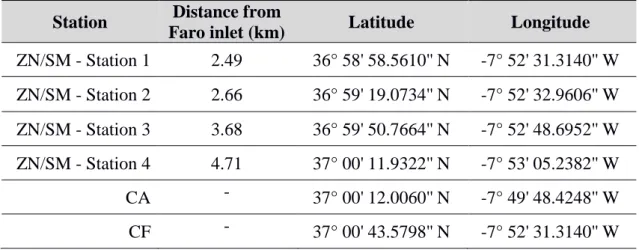
Table 2.1 - Geographical description of the sampling stations. ZN: Zostera noltei, SM: Spartina maritima, CA: Caulerpa prolifera, CF: Clam Farm.

Station Distance from

Faro inlet (km) Latitude Longitude

ZN/SM - Station 1 2.49 36° 58' 58.5610'' N -7° 52' 31.3140'' W ZN/SM - Station 2 2.66 36° 59' 19.0734'' N -7° 52' 32.9606'' W ZN/SM - Station 3 3.68 36° 59' 50.7664'' N -7° 52' 48.6952'' W ZN/SM - Station 4 4.71 37° 00' 11.9322'' N -7° 53' 05.2382'' W CA - 37° 00' 12.0060'' N -7° 49' 48.4248'' W CF - 37° 00' 43.5798'' N -7° 52' 31.3140'' W

2.2 Vegetation’s properties

A description of the ZN and SM stations was performed during a 1-day campaign (13th_{of January 2017) at low tide. Vegetation properties determined for Z. noltei and S.} maritima were: shoot density (shoots m-2_{), canopy height (cm), above-ground biomass (g} DW m-2_{), below-ground biomass (g DW m}-2_{) and an index of the canopy area per unit of}

(29)

13 sediment surface area, i.e. the leaf area index (LAI, for ZN) and LAI plus stem area (for SM).

Replicated quadrates (n = 3) were haphazardly positioned in each sampling location and vegetation in the corresponding area was extracted, ensuring that all the tissue below and above ground was included. The area of the quadrats was selected based on the species being sampled: Z. noltei = 10×10 cm (100 cm2); S. maritima = 28×28 cm (784 cm2). Tissue samples were rinsed of sediment in situ and brought to the laboratory, where they were frozen at -20ºC until processing.

When processing samples, vegetal tissue was repeatedly rinsed and manually selected until all material not belonging to the target species had been removed. Total number of shoots was counted and five shoots were selected to measure total length and area. Areas were measured by scanning followed by image processing in ImageJ1.51n (Schneider et al., 2012). LAI and stem areas could then be calculated as:

(1) Leaf area index (m2 m-2) = Leaves per shoot × Shoot density (shoots m-2) × Shoot area (m2_shoot)

(2) Stem area (m2_{) =}_{π × Projected stem area (m}2₎

Biomass was then separated in above ground (leaves for ZN, leaves + stems for SM) and below ground (roots and rhizomes), dried in an oven at 60ºC until constant weight (4 to 5 days) and weighted (dry weight, g DW).

2.3 Organic matter sources collection

Samples of the potentially most important sources of organic matter to these ecosystems were collected during January and February of 2017. Four main sources were selected: suspended particulate organic matter (SPOM), Z. noltei tissue, S. maritima tissue and macroalgae that formed mats in both areas (Ulva sp. plus epiphytes).

SPOM samples were obtained by collecting 1 L of superficial seawater near each station, in the middle of the channel. Water samples were filtered using a vacuum pump system through glass microfiber filters (GF/F, 47 mm). After sample filtration, filters were rinsed with distilled water to remove salts and ensure that all particles were removed

(30)

14

from the filtration cup. Filters were carefully removed and stored in identified petri dishes which were frozen at -20ºC, lyophilized for 24 hours and stored until further analysis.

Replicated samples (n = 3) of Z. noltei and S. maritima were cleaned of epiphytes and sediments, rinsed with distilled water, separated into above and below-ground tissues and then frozen (-20ºC) until sample processing. Later they were lyophilized for 24 hours, pulverized in a ball-mill (with agate material to avoid contamination) and sent for elemental and isotopic analysis.

2.4 Core extraction, description and sub-sampling

Sediment cores were extracted from the sampling locations from 30 of January to 16 of February of 2017. An area within the vegetation patch was selected to avoid edge effects. Core samplers consisting of sharpened PVC pipes (length = 170 cm; ø = 5cm) were manually hammered into the seafloor until penetration was no longer possible, or a depth of 160 cm was reached. The difference between the core sampler’s upper mouth and the seafloor was measured (extra – e) for further calculations (Figure 2.3). A styrofoam plug was then inserted in the upper part of the sampler until the surface of the sediment core was reached and the sampler was sealed at the top (using a rubber stopper) to restrict air flow. A raised pulley system supported in platforms was used to extract the core. Bottom of the sampler was checked for any loss of sediment during the uplift and the height of the amount lost (lost – L, Figure 2.3) was measured with a ruler. Sediment cores were transported carefully to the laboratory for immediate processing.

In the laboratory, core samplers were longitudinally cut in half using a mechanical saw and cores were halved with a wire saw. The height of the sediment core was measured (height – h, Figure 2.3) with a metric tape (±0.1 cm).

Core compaction was visually appreciable during its extraction. The compaction rate was calculated for each core assuming linear compression (equation 8) (Glew et al., 2001) based on the measures taken during core extraction. All measured volumes and depths along each core were corrected by dividing them by the compaction correction factor (equation 7) of that specific core.

(31)

15

Figure 2.3 - Schematic of measurements used to calculate and

correct compaction.

(3) Penetration depth (p) (cm) = 170 – e

(4) Compaction correction factor (Ccorr) = h+L

p

(5) Compaction rate = (1 – Ccorr) × 100

One half of the core was photographed and visually described by determining layers of similar sediment lithology and horizons delimiting such layers. Presence of organisms and organic structures was also noted (symbology adapted from Li et al. 2015). Sediment color measurements (n = 3) were performed every 1 cm using an X-Rite Colortron II spectrophotometer, after covering the core surface in plastic wrap to prevent sediment from adhering to the equipment (no significant effect of plastic wrapping on color measurements has been proved in preliminary tests). The core was then sliced and sub-sampled every 2 cm using a Teflon spatula. During sampling, the sediment near the corer was avoided to prevent potential contamination by transported materials along the sampler walls during the core extraction. Samples were placed in identified zip-lock bags and frozen at -20ºC until further processing (group A samples).

The second core half was also divided in slices every 2 cm. First, a sub-sample from each slice was taken using a syringe (diameter of 1.5 cm). Volume of the sample (Sample Volume, cm3) was measured in the syringe graduation (±0.1 mL) and the sample was placed in an identified zip-lock bag (group B samples). The remaining sediment in the slice was sampled into a separated zip-lock bag (group C samples). All samples were then frozen at -20ºC for storage.

(32)

16

2.5 Sediment properties analysis

2.5.1 Sample selection

A series of samples along each core was selected for further analysis. Two selection criteria were used, based on the depth of the samples:

a) Samples in the top 50 cm of depth: select every other slice;

b) Samples over 50 cm of depth: select the second sample before and after each horizon, so that the start and end of each sedimentary layer were measured. If a layer was over 30 cm long, a middle sample was also selected. Layers under 5 cm of length were disregarded. When samples with high content of shell fragments were selected, another sample was selected deeper within the layer.

2.5.2 Porosity, dry bulk density and organic matter fraction

Porosity, dry bulk density (DBD) and organic matter fraction were determined in sub-samples B. Because these are flooded sediments, porosity (equation 7) and DBD can be determined based on the moisture content (Avnimelech et al., 2001). Frozen samples were weighted (Weightinitial, g) in a micro-balance (±0.0001 g), lyophilized (24 h) and weighted again (Weightdry, g). The DBD was calculated as the ratio between the dry weight and the sample volume (equation 7).

(6) Porosity (%) = Weightinitial(g)−Weightdry(g)

Weightinitial(g) × 100

(7) Dry bulk density (g cm-3_{) =} Weightdry(g)

Sample Volume(cm3₎

Sediment samples were then ground in a ball mill using agate material until a fine and homogenous powder was obtained. Approximately 0.5 g of the ground samples were stored in identified Eppendorf tubes for isotopic analysis. The remaining ground sample was weighted (Weightdry, g), placed in an aluminum foil cup and used to estimate the organic matter content by Loss on Ignition (LOI) (equation 8), I.e. by combusting the sample at 450ºC for 4 hours (Heiri et al., 2001).

(33)

17

(8) Organic matter content (%) = Weightdry (g)-Weightcombusted (g)

Weightdry (g) × 100

The OM content and DBD were then used to calculate the sediment OM concentration (equation 9), which gives the amount of OM per unit of sediment volume.

(9) OM concentration (g OM cm-3_{) =}_{OM content (%) × Dry Bulk Density (g cm}−3₎

2.5.3 Elemental and isotopic analysis

Organic carbon content (Corg, % dry weight) and δ13Corg (vs VPDB) were analyzed in the sediment samples after carbonate removal by direct addition of 1 M HCl until the reaction was complete. Total nitrogen content (Ntotal, % dry weight) and δ15_{N (vs Air)} were analyzed in untreated samples. Isotopic signatures were also analyzed in the dry tissues of the sources selected for the mixing models (section 2.3). Organic carbon content analysis was performed by high temperature combustion NDIR detection (method reference: EPA 415.1; instrument: Shimadzu TOC-V). Total nitrogen content was analyzed by high temperature combustion chemiluminescence detection (method reference: ASTM D5176; instrument: Shimadzu TNM-1). Both δ13Corg and δ15N were analyzed by Isotope Ratio Mass Spectrometry (instrument: Thermo DeltaV). Sample treatment and analysis was performed by UH Hilo Analytical Laboratory (Hawaii, USA). Values of elemental concentrations under detection limit were assumed to be 0.

Organic carbon and total nitrogen contents were used in conjunction with dry bulk density to calculate sediment Corg and Ntotal concentrations (g element cm-3, equation 10).

(10) Element concentration (g element cm-3_{) =}_{element content × DBD}

Corg and Ntotal concentration were integrated along the core depth (standardized to 100 cm) to calculate the storage capacity of each habitat (g element cm-2), i.e. the Corg or Ntotal stock per area. Approximate integral values were calculated using linear interpolation (Ekstrøm, 2017).

(34)

18

2.6 Stable Isotopic Mixture Models

Stable isotopic mixture models were calculated using SIMMR library from R (Parnell, 2016), utilizing four main sources of organic matter: suspended particulate organic matter (SPOM); macroalgae (MA), S. maritima (SM) and Z. noltei (ZN).

Samples that were considered to have suffered changes in signatures due to diagenesis were excluded. This evaluation was performed separately for carbon and nitrogen: 1) low Corg contents were associated with a lower δ13Corg, suggesting that degradation of organic matter in those samples affected δ13_{Corg; 2) low Ntotal was related} to an increase in the variance of δ15_{N, once again suggesting possible alterations due to} organic matter degradation. Samples with the largest alterations were excluded in both cases (i.e low δ13Corg plus low Corg content; low Ntotal content plus high deviance from mean value) (Annex 1).

2.7 Sediment color

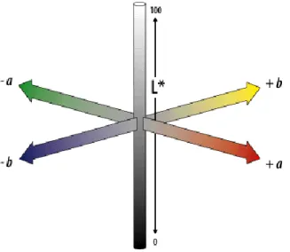
Sediment color was measured and analyzed in CIELab color space. Designed to be in accordance with the Munsell color system typically used for soil characterization (Koschan & Abidi, 2008; Wills et al., 2007), this system characterizes colors using three dimensions: lightness (L*, where 0 equals to black and 100 equals to diffuse white); red-green (a*, negative values correspond to red-green, positive values correspond to red); yellow-blue (b*, negative values correspond to blue, positive values correspond to yellow)(Figure 2.4) (Adobe Systems Incorporated, 2000).

Figure 2.4 - CIELAB color space dimensions. The color space uses 3 dimensions to describe color: L* (lightness); a* (green-red) and b* (blue-yellow). (Adobe Systems Incorporated, 2000).

(35)

19

2.8 Statistical analysis

2.8.1 Vegetation description

Differences of vegetation parameters amongst stations (1 to 4) within each habitat (ZN and SM), or differences between habitats (ZN and SM) were tested by one-way ANOVA (when assumptions of normality and homoscedasticity were met) or Kruskall-Wallis (when assumptions were not met). Differences between groups were tested using TukeyHSD multiple comparison test (for ANOVA) or Dunn’s test (for Kruskall-Wallis). Effects were considered significant at p < 0.05.

2.8.2 Sedimentary Corg content

Stepwise regression analysis (bidirectional elimination) was performed to select the best model to predict Corg. The full model included Habitat, Station, Depth, Habitat:Depth interaction and Station:Depth interactions. Another analysis with log10-transformed Depth was also done. Addition and removal of predictors was performed and subsequent model performance was compared based on AIC (Akaike Information Criterion, Akaike (1974), with the lowest AIC corresponding to the best model). Pair-wise comparisons were performed on the marginal means of the selected model to test for significant differences Corg contents between sampled cores (Tukey's HSD). Differences were considered significant at p < 0.05.

2.8.3 Organic matter sources

The effect of hydrodynamics (stations 1 – 4) on the theoretical contribution of the sedimentary organic matter sources (obtained from the stable isotopic mixture models, section 2.6) was tested with a two-way ANOVA, using source and station as main factors (after testing assumptions of normality and homoscedasticity). Effects were considered significant at p < 0.05.

2.8.4 Organic matter as proxy for Corg and Ntotal

Correlation analysis (Pearson's coefficient, r) was performed to test association between organic matter and Corg/Ntotal. One-way ANCOVA was used to test for significance of Habitat (main factor) and organic matter (covariate) (effects were

(36)

20

considered significant at p < 0.05). Linear regressions were then constructed to predict Corg or Ntotal based on ANCOVA results.

2.8.5 Sediment color as proxy for organic matter

Stepwise regression analysis (bidirectional elimination) was performed to select the best model to predict organic matter based on color measurements. The full model included Habitat, L*, a* and b* and all 2-way interactions. Another analysis with log10-transformed organic matter was also done. Addition and removal of predictors was performed and model performance was compared based on AIC (Akaike Information Criterion, Akaike (1974), with the lowest AIC corresponding to the best model).

(37)

21

3 R

ESULTS

3.1 Vegetation description

All vegetation properties except canopy area were significantly different between Z. noltei meadows and S. maritima saltmarshes (Table 3.1). Shoot density in Z. noltei was higher than in S. maritima. Canopy height, above ground biomass and below ground biomass were all lower in Z.noltei meadows (Table 3.1).

Table 3.1 - Summary (mean +/- SD) of the structural variables of Zostera noltei and Spartina maritima averaged across all sampling stations. Results of the 1-way ANOVA (F; Shoot density, Canopy area, Canopy height) or Kruskal-Wallis test (χ2; AG biomass, BG biomass) are presented, indicating whether the differences across habitats were significant (ns: not significant, *** p < 0.001, ** p < 0.01, * p < 0.05). Superscript lettering represent post-hoc pairwise comparisons indicating differences among the stations. (AG: Above ground, BG: Below ground; DW: dry weight; df: degrees of freedom).

Variable S. maritima Z. noltei Test (df = 1)

Shoot density (shoots m-2₎ 772.75 ± 269.56 10450.00 ± 4974.75 x2 17.29*** Canopy area (shoots m-2₎ 1.82 ± 0.85 2.68 ± 1.54 F = 2.88ns Canopy height (cm) 27.83 ± 11.00 8.95 ± 3.92 F = 31.36*** AG biomass (g DW m-2₎ 266.90 ± 154.28 35.39 ± 22.97 x2 = 17.29*** BG biomass (g DW m-2₎ 1093.38 ± 695.34 267.39 ± 133.59 x2 = 11.21 ***

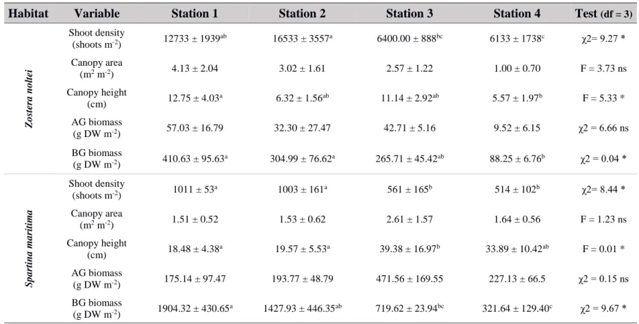
From the five vegetation properties measured, three varied significantly along the hydrodynamic gradient in both S. maritima and Z. noltei (Table 3.2). Below-ground biomass and shoot density decreased along the hydrodynamic gradients in both species, being highest at the more exposed station (station 1) and lowest at the most sheltered one (station 4). In S. maritima this was accompanied by an increase in canopy height from the two most exposed stations to the two most sheltered. No trend was observed in Z. noltei canopy height, despite significant differences amongst stations (Table 3.2). Canopy area and above ground biomass did not display significant differences amongst sampled stations.

(38)

22

Table 3.2 - Summary (mean +/- SD) of the structural variables of Zostera noltei and Spartina maritima at the four locations sampled, from the closest to the inlet (1) to the furthest (4). Results of the 1-way ANOVA (F; Shoot density, Canopy area, Canopy height) or Kruskal-Wallis test (χ2; AG biomass, BG biomass) are presented, indicating whether differences across stations were significant (ns: not significant, *** p < 0.001, ** p < 0.01, * p < 0.05). Superscript lettering represent post-hoc pairwise comparisons indicating differences among the stations. (AG: Above ground, BG: Below ground; DW: dry weight; df: degrees of freedom).

Habitat Variable Station 1 Station 2 Station 3 Station 4 Test (df = 3)

Z o stera no ltei Shoot density (shoots m-2₎ 12733 ± 1939ab 16533 ± 3557a 6400.00 ± 888bc 6133 ± 1738c χ2= 9.27 * Canopy area (m2_m-2₎ 4.13 ± 2.04 3.02 ± 1.61 2.57 ± 1.22 1.00 ± 0.70 F = 3.73 ns Canopy height (cm) 12.75 ± 4.03 a _{6.32 ± 1.56}ab _{11.14 ± 2.92}ab _{5.57 ± 1.97}b _{F = 5.33 *} AG biomass (g DW m-2₎ 57.03 ± 16.79 32.30 ± 27.47 42.71 ± 5.16 9.52 ± 6.15 χ2 = 6.66 ns BG biomass (g DW m-2₎ 410.63 ± 95.63a 304.99 ± 76.62a 265.71 ± 45.42ab 88.25 ± 6.76b χ2 = 0.04 * Sp a rtin a m a ritima Shoot density (shoots m-2₎ 1011 ± 53a 1003 ± 161a 561 ± 165b 514 ± 102b χ2= 8.44 * Canopy area (m2_m-2₎ 1.51 ± 0.52 1.53 ± 0.62 2.61 ± 1.57 1.64 ± 0.56 F = 1.23 ns Canopy height (cm) 18.48 ± 4.38 a _{19.57 ± 5.53}a _{39.38 ± 16.97}b _{33.89 ± 10.42}ab _{F = 0.01 *} AG biomass (g DW m-2₎ 175.14 ± 97.47 193.77 ± 48.79 471.56 ± 169.55 227.13 ± 66.5 χ2 = 0.15 ns BG biomass (g DW m-2₎ 1904.32 ± 430.65a 1427.93 ± 446.35ab 719.62 ± 23.94bc 321.64 ± 129.40c χ2 = 9.67 *

(39)

23

3.2 Sedimentary profile description

Cores extracted using 170 cm samplers (ZN and SM) reached sampling depths ranging from 108 to 160 cm (Table 3.3). The core in station CA reached a sampling depth of 56.5 cm. Compaction rates observed ranged from 14.4% to 43.8% (Table 3.3).

Table 3.3 – Core height, sampling depth, compaction correction factor and compaction rates of extracted cores in each location. Core height is the total height of the core, as measured inside the core sampler. Sampling depth refers to the depth reached by the end of each core, after correction due to compaction. Location names abbreviations: CA – Caulerpa prolifera; CF – Clam Farm; SM – Spartina maritima; ZN –

Zostera noltei; 1 – 4 – Station.

Location Core height (cm) Sampling depth (cm) Compaction correction factor (%) Compaction rate (%) CA 45 56.5 80.8 19.2 CF 124 145.0 85.5 14.5 SM1 111 134.5 82.5 17.5 SM2 85 108.0 78.7 21.3 SM3 112 160.0 70.0 30.0 SM4 90 160.0 56.3 43.8 ZN1 95 126.7 75.0 25.0 ZN2 98 128.2 76.5 23.6 ZN3 92 140.2 65.6 34.4 ZN4 88 119.8 73.4 26.6

Visual description of the cores is presented in Figure 3.5. The sediment beneath Caulerpa prolifera (CA) had two superficial layers of clay, with shells and shell fragments in the first one. These two layers formed the initial 37.1 cm of the core, after which it transitioned to sandy sediment. In the clam farm core (CF), sand constituted most of the core, except for one layer of clay between 26.9 cm and 45.6 cm.

SM and ZN sediment showed a similar trend in how they vary along the hydrodynamic gradient. In general, the clay fraction of the SM and ZN sediment increases as the hydrodynamic energy of the station decreases. In station 1 (SM1), the highest energy environment, there was a superficial clay layer (13.3 cm), before transitioning to sand. Entering the tributary channel, station 2, SM2 showed a similar superficial clay layer, followed by silt from 14 to 66 cm, and another clay layer at the end. SM3 had two clay layers that extended to 101.4 cm of depth, while SM4’s clay layers were continuously found until 145.8 cm. ZN1 had an initial clay layer, before transitioning to silt (at 30.7

(40)

24

cm) and then sand (at 61.3 cm). ZN2 has a shallower superficial layer than ZN1, but transitions into silt and then again into clay, showing its first sandy layer at a depth of 85 cm. ZN3 was constituted of clay sediment in its entirety (140.2 cm) and ZN4 until 85.8 cm, after which it transitions to sandy sediment.

(41)

25

Figure 3.5- Visual descriptions of the sediment cores and symbology used. Location names abbreviations: CA – Caulerpa prolifera; CF – Clam Farm; SM – Sparina maritima; ZN – Zostera noltei; 1 – 4 – Station.

(42)

26

3.3 Sedimentary Corg and Ntotal: variation along hydrodynamic gradient

The median values for Z. noltei and S. maritima sedimentary Corg contents, 1.31% and 1.11%, respectively were not significantly different from each other (Figure 3.6a). They were, however, significantly higher than both C. prolifera’s and the clam farm, which had median values of 0.50% and 0.23%, respectively. The same trend was observed for Ntotal (Figure 3.6b), where the median values for Z. noltei and S. maritima were significantly higher than for C. prolifera and clam farm.

Figure 3.6 - Sedimentary organic carbon (A) and total nitrogen (B) content in sampled habitats. Boxplots components from middle out: thick line inside the boxes represents the median; boxes extend from 25th to 75th percent quantile; whiskers extend up to 1.5 x IQR; values outside of the whisker’s range are considered outliers and plotted as dots. Lettering above the boxes represents homogenous groups (p < 0.05, Dunn’s test). Location names abbreviations: CA – Caulerpa prolifera; CF – Clam Farm; SM – Sparina maritima; ZN – Zostera noltei; 1 – 4 – Station.

Considering a sediment depth of 100 cm, the amount of Corg per area of habitat in SM and ZN was not significantly different (0.80 ± 0.36 and 0.81 ± 0.26 g Corg cm-2_, respectively) (Figure 3.7). Ntotal storage did not differ either for SM and ZN (0.082 ± 0.040 and 0.087 ± 0.019 g Ntotal cm-2_{, respectively). Stocks of Corg (0.36 g Corg cm}-2_{) and} Ntotal (0.044 g Ntotal cm-2_{) in the clam farm were lower than the two vegetated intertidal} habitats (Figure 3.7).

(43)

27

Figure 3.7 – Organic carbon (A) and total nitrogen (B) storage per area of habitat. Values were calculated from the sediment surface to a depth of 100 cm. ZN and SM are averaged over the 4 sampled locations. Location names abbreviations: CF – Clam Farm; SM – Sparina maritima; ZN – Zostera noltei.

In general, Corg decreased over sediment depth (Figure 3.8). In Z. noltei and S. maritima sediment, this decrease was more accentuated at shallow depths and then stabilized (Figure 3.8).

The clam farm sediment showed less variation in Corg content. Throughout the profile, values remained below 0.33%, except for sediment between 19.9 and 43.3 cm, where values up to 0.89% were measured (Figure 3.8). This depth partially coincides with the change from sand to clay (Figure 3.5, Annex 2).

The depth variation of Corg in S. maritima stations 1 and 2 was similar, ranging from 3.1% to 4.8% for the first 10 cm, whereas in stations 3 and 4 it ranged from 2.2% to 2.9%, also in the first 10 cm. A sharp decline is then seen on stations 1 and 2, to values from 0.02% to 0.37%, from 15 to 65 cm of depth, coincident with the change from clayey to sandy sediment (Annex 2). After 65 cm, a strong increase was observed, more accentuated and coincident with a return to clayey sediment in SM2 (Annex 2). Stations 3 and 4 showed a decrease in Corg content after the initial 10 cm until the end of the cores, when %Corg reached a minimum of 0.09% and 0.58%, respectively. Station 4 also showed a relevant increase from 1.3% at 80 cm to 2.7% at 87.1 cm. At depths higher than 125 cm, the Corg within S. maritima sediment tended to approach 0% (Figure 3.8).

The depth variation of Corg in Z. noltei showed very similar trends across stations, ranging from 0.5% to 1.57% for the first 12 cm in stations 1 and 2. Corg in stations 3 and