USING R TO TEACH SEASONAL ADJUSTMENT
Pedro Costa Ferreira
Brazilian Institute of Economics (FGV/IBRE) [email protected]
Daiane Marcolino de Mattos
Brazilian Institute of Economics (FGV/IBRE) [email protected]
Abstract
This article shows, using R software, how to seasonally adjust a time series using the X-13-ARIMA-SEATS program and the seasonal package developed by Christoph Sax. In addition to presenting step-by-step seasonal adjustment, the article also explores how to analyze the program output and how to forecast the original and seasonally adjusted time series. A case study was proposed using the Brazilian industrial production. It was verified that the effect of Carnival, Easter and working days improved the seasonal adjustment when treated by the model.
Keyword: Seasonal Adjustment, X-13ARIMA-SEATS, R software, RStudio
1. Introduction
A time series, according to the classical decomposition, can be broken down into four unobservable components: trend, seasonality, cycle and irregularities. Seasonality, the main object of this study, is caused by oscillatory movements of the same frequency that occur in an intra-annual period, such as climatic variations, vacation, holidays and more.
The occurrence of these events can lead to inappropriate conclusions about the time series under study. For example, the offer of employment typically increases at the end of the year due to the Christmas holidays, that is, there is a greater demand for goods and services, raising the level of staff hiring. However, as the majority of these vacancies are temporary (seasonal), generally there is a decrease in the level of staff employed in the following period. For an economic analysis, the important thing is to detect the difference between what occurs periodically and what actually occurs differently in that specific period, allowing one to observe the trend and the variable cycle.
For this, you need a suitable tool that can remove this component (seasonality). Removing the seasonality from a time series is called 'seasonal adjustment' or 'deseasonalization'. In the literature one can find several methodologies/software that allow the removal of the seasonality of a time series.
To do that we are going to use the R software (R Core Team, 2015). So, it’s recommended that the user has already worked with this program. Some books and articles that can be useful for this propose are: A Computer Evolution in Teaching Undergraduate Time Series (Hodgess, 2004); Fun with the R Grid Package (Zhou & Braun, 2010); An Introduction to R (R Core Team, 2015); R in a Nutshell (Adler, 2009); A First Course in Statistical Programming with R (Braun & Murdoch, 2008); Introductory Statistics with R (Dalgaard, 2008); Análise de Séries Temporais em R – um curso introdutório (Ferreira, Mattos, Oliveira, Lima, & Duca, 2016).
In this context, the aim of this paper is to present how we can make a seasonality adjustment using the X-13ARIMA-SEATS interface in the R/RStudio. To achieve this goal, in addition to this introduction, the paper is organized as follows: in the next section we briefly present the X13 program and suggested steps to adjust the seasonality. In section 3 we run the seasonal adjustment steps in R. Finally, in section 4, we draw conclusions and discuss the evolution of the work.
2. Seasonal adjustment methodology
It is important that the reader knows there are many ways to make the seasonal adjustment. Some examples are: Regression Models with dummy variables and Exponential Smoothing Models. In this article, however, we use the X-13ARIMA-SEATS, referred to as just X13 from now on.
The X13 was developed by the U.S. Census Bureau with the support of the Bank of Spain. The program, created in July 2012, is the junction of two other seasonal adjustment programs: X12-ARIMA (Findley et al, 1998) and TRAMO/SEATS (Gómez & Maravall, 1996). Besides seasonal adjustment, the program offers several diagnoses which allow the user to evaluate the quality of seasonal adjustment.
Another X13 procedure that deserves mentioning is the pre adjustment of the time series, that is, a kind of correction made before the seasonal adjustment. Some atypical and/or non-seasonal events, for example calendar effects (trading days, working days, moving holidays), strikes, disasters, among others, may affect the seasonal parameter estimation, and consequently a low quality seasonal adjustment will be generated. These kinds of events must be treated (pre adjustment) if necessary. Another important procedure of X13 is the use of ARIMA models to forecast the time series. It is essential that the model is well diagnosed, otherwise forecast errors can be significant.
On the program developers website (United States Census Bureau, 2016) there are a lot of books, articles and tutorials that may be useful to the user who wants to delve deeper into this topic, such as the program manual: X-13ARIMA-SEATS Reference Manual Accessible HTML Output (United States Census Bureau, 2015). Other articles recommended by the authors and available at the website are Historical Papers Concerning X-11 and Seasonal Adjustment (United States Census Bureau, 2015). However, it’s important to know that in this article all the steps required to perform a good seasonal adjustment will be presented. To perform the seasonal adjustment in R, we use the following steps:
Graphical Analysis;
Implementation of X-13ARIMA-SEATS in automatic mode;
Evaluation of seasonal adjustment in (2);
Forecast.
The graphical analysis of a time series allows you to visualize your features for good modeling. For example: its seasonal pattern, structural breaks, possible outliers, whether it’s necessary to make a logarithm transformation in the time series to stabilize the variance, etc. To evaluate the quality of the seasonal adjustment, the X13 offers some tools such as seasonality tests, autocorrelation tests, normality and graphs to verify the seasonality factors stability. If there are some flaws in a diagnosis, the setting can be redone without using automatic options. It’s important to know that tools to help the seasonal adjustment but the article will not explore all of them.
3. How to make the seasonal adjustment in R
Before presenting the tutorial on how to make seasonal adjustment with X13 in R, it is essential to know that over time the R packages and functions may be updated and consequently may not work as presented in this tutorial. So we highlight the versions of the programs and packages used during this article, beginning with the version of the main program: R versão 3.2.3 e RStudio versão 0.99.491.
3.1 Preparing the working environment1
The five steps mentioned in section 2 are suggested for a quality seasonal adjustment. To run them in R, however, some procedures need to be executed first:
a) Define the working directory:
b) Download the X-13ARIMA-SEATS executable file;
c) Inform the location of the executable file downloaded in (2); d) Install and load the seasonal package;
e) Verify whether the previous steps were executed correctly; f) Read the time series you are interested in.
The steps are presented below:
a) Define working directory: the input files required to make the seasonal adjustment to the time series which you are interested in and the X-13ARIMA-SEATS
1 It’s important to highlight that all the codes are available at
executable file will be here. The reader may place the working directory in any folder. In this example, we place the working directory in the folder called “work”:
> setwd("C:/work")
b) Download the X-13ARIMA-SEATS executable file: The software can be downloaded at the U.S. Census Bureau website. It must be downloaded and placed in the working directory folder defined in Step 1. An easier way, by following the commands below you can get the file directly from the R environment. The file will be stored in the working directory specified above with the name x13.zip, and then unzipped. The X13 version used here is version 1.1.
> download.file("https://www.census.gov/ts/x13as/pc/x13as_V1.1_B19.zip", + destfile = "./x13.zip")
> unzip("x13.zip")
Occasionally, new versions of the program may be created causing changes on the download link and hence the command line may not work. It’s important to remember that it’s not necessary to download the executable file every time the seasonal adjustment is done. Leave it in the working directory for future use and proceed to the next step.
c) Inform the location of the executable file downloaded in (b): The x13as.exe file is the one which actually does the seasonal adjustment, so it’s important to inform its path to R.
> local <- paste0(getwd(), "/x13as") > Sys.setenv(X13_PATH = local)
d) Install and load the seasonal package: Christoph Sax (2015) developed the seasonal package that runs the X-13ARIMA-SEATS in R. The package must be installed and loaded. This article uses the version 1.1.0.
> install.packages("seasonal") > library(seasonal)
e) Verify whether the previous steps were executed correctly: the checkX13() function from the seasonal package allows you to verify whether it is possible to make the seasonal adjustment. If the four previous procedures were performed correctly, the function returns a confirmation message and it is possible to make the seasonal adjustment with the X-13ARIMA-SEATS in R.
f) Read the time series you are interested in: we will seasonally adjust the Brazilian industrial production index (base 2012 = 100), produced and released by the Brazilian Statistics Bureau (IBGE, 2015). The database range is from Jan 2002 to Dec 2014. To make our life easier we are going to download the database straight from the Github platform. After, we’ll transform the database into the time series object, as presented below. > install.packages("RCurl") > library(RCurl) > usingR_url <- getURL("https://raw.githubusercontent.com/pedrocostaferreira/Articles/master/using-R-to-teach-seasonal-adjustment/IPI.csv")
> ipi <- ts(read.csv2(text = usingR_url), start = c(2002,1), freq = 12)
Once the work environment is ready, we are able to go to the next step: seasonally adjust the interested time series.
3.2 Graphical Analysis
An easy way to see a time series line chart is using the plot() function. Another chart that can help understand the time series behavior is given by the monthplot() function. This chart outlines the time series from each month which helps to identify seasonal patterns. Below you can see the R command.
> # Figure 2 > plot(ipi)
> abline(h = seq(70,110,5), v = seq(2002,2015,1), lty = 3, col = "darkgrey") > # Figure 3
> monthplot(ipi, labels = month.abb, lty.base = 2)
> legend("topleft", legend = c("ipi/month", "average/month"), + cex = 0.8, lty = c(1,2), bty = "n")
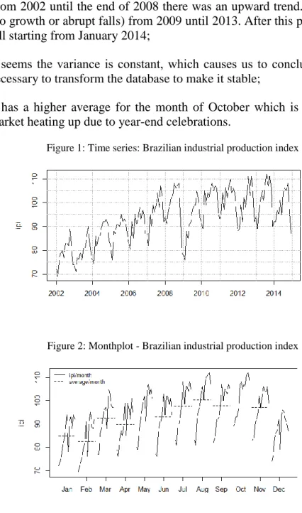
The chart analysis (Figures 1 and 2) allows us to assume important points about the Brazilian industrial production:
Seasonal behavior, from March to October the index has increased while in the other months, decreased. This behavior is repeated every year;
an atypical behavior during this period, which can be understood as an outlier;
From 2002 until the end of 2008 there was an upward trend. It seems stable (no growth or abrupt falls) from 2009 until 2013. After this period it shows a fall starting from January 2014;
It seems the variance is constant, which causes us to conclude that it’s not necessary to transform the database to make it stable;
It has a higher average for the month of October which is justified by the market heating up due to year-end celebrations.
Figure 1: Time series: Brazilian industrial production index
Figure 2: Monthplot - Brazilian industrial production index
3.3 Implementation of X-13ARIMA-SEATS in automatic mode
After we observe graphically the time series behavior, the next step is to run the seasonal adjustment in the automatic mode. We can then check, for instance, if the X13 program identifies some of the months at the end of 2008 as outliers, as we observed graphically.
To run the seasonal adjustment you should use the seas() function from the seasonal package. The function has a lot of arguments. However, as our goal now is just
to make the seasonal adjustment in the automatic model, we will use just the argument x which indicates the time series to seasonally adjust.
> seas_adjust <- seas(x = ipi)
3.4 Verify whether the previous steps were executed correctly This step consists of four basic procedures:
a) Verify the Seasonality QS test;
b) Pre-adjustment diagnosis and SARIMA model;
c) Verify the seasonality evidence or working days effect graphically; d) Seasonal adjustment stability;
It is important to check the seasonality of the time series since without evidence of seasonality, time series should not/cannot be adjusted. In addition, it is expected that the seasonal pattern disappears after seasonal adjustment. Although this seems obvious, empirical studies have shown that not all automatic adjustments were able to remove the seasonality as was expected. So it is really important to evaluate the test for seasonality.
The X13 seasonality test is given by the QS statistic. The null hypothesis of the test is no seasonality. When the time series has more than eight years of information (as in the case of this study), the test is done in the complete series and with the last [most recent] 8 years. Otherwise the test is done only in the full series. Besides being applied in the original series and the seasonally adjusted time series, the test is also applied to the ARIMA model residuals and the irregular component. Except in the original time series, we expect no evidence of the seasonality in all other time series.
In R, we use the qs() function from the seasonal package to run the test. The results can be seen below:
> qs(seas_adjust) qs p-val qsori 162.6689 0 qsorievadj 236.5394 0 qsrsd 0.02387 0.98814 qssadj 0 1 qssadjevadj 0 1 qsirr 0 1 qsirrevadj 0 1 qssori 81.40339 0 qssorievadj 136.5975 0 qssrsd 0 1 qsssadj 0 1
qsssadjevadj 0 1
qssirr 0 1
qssirrevadj 0 1
As we can observe, when considering a confidence level of 95%, there is no evidence of seasonality in the seasonally adjusted time series, residuals and the irregular component, and there is evidence of seasonality in the original time series. These results are similar to the test applied to the last 8 years (second part of the qs() function output2). The next step is pre-adjustment diagnosis and SARIMA model. To do this, we’ll use the summary() function.
> summary(seas_adjust) Call:
seas(x = ipi) Coefficients:
Estimate Std. Error z value Pr(>|z|) Mon 0.0055494 0.0023373 2.374 0.0176 * Tue 0.0053673 0.0023757 2.259 0.0239 * Wed 0.0022694 0.0022926 0.990 0.3222 Thu 0.0052843 0.0023300 2.268 0.0233 * Fri 0.0004402 0.0023069 0.191 0.8487 Sat -0.0002930 0.0023159 -0.127 0.8993 Easter[1] -0.0242646 0.0043734 -5.548 2.89e-08 *** LS2008.Dec -0.1334385 0.0182778 -7.301 2.87e-13 *** AO2011.Feb 0.0612578 0.0129029 4.748 2.06e-06 *** AO2014.Feb 0.0629949 0.0140520 4.483 7.36e-06 *** MA-Seasonal-12 0.6797172 0.0694161 9.792 < 2e-16 *** --- Signif. codes: 0 ‘***’ 0.001 ‘**’ 0.01 ‘*’ 0.05 ‘.’ 0.1 ‘ ’ 1 SEATS adj. ARIMA: (0 1 0)(0 1 1) Obs.: 156 Transform: log AICc: 613.8, BIC: 646.9 QS (no seasonality in final): 0 Box-Ljung (no autocorr.): 23.4 Shapiro (normality): 0.9817 *
The summary() function output shows that the pre-adjustment used calendar variables such as Easter (Easter[1]) and weekdays (Mon, Tue, etc). All the variables are significant taking into account a significance level of 5%. Even if only some week day variables are significant, this suggests that the amount of weekdays in the month influences the Brazilian industrial production. However, it’s important to know that the
2 qsori: original series; qsorievadj: original series extreme-value adjusted; qsrsd: ARIMA residuals;
calendar variables were not built based on the Brazilian calendar, hence, it must be modified.
Outliers have also been detected: a level shift outlier in December 2008 (LS2008.Dec), month affected by World Crisis, and 2 additive outliers, both unexpected by graphic inspection, on February 2011 and 2014 (AO2011.Feb e AO2014.Feb). Both outliers are statistically significant, at 5% level. In order to better understand the types of outliers implemented in X13, we suggest the Eurostat (2016) tutorial.
The estimated ARIMA model is of an order of magnitude (0 1 0)(0 1 1), and the seasonal MA parameter is significant. According to the Ljung-Box autocorrelation test, there is no evidence of residual autocorrelation for the estimated ARIMA model. The Shapiro-Wilk normality test suggests non-normality. However, this is not an extremely necessary characteristic for the ARIMA models diagnosis. Note that the data logarithm transformation was also employed, despite the fact it was not expected in the graphic analysis.
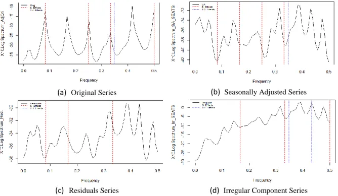
The next diagnosis provided by the application is focused on verifying whether there is evidence of seasonality and working days effects before and after seasonal adjustment. The diagnosis is yielded by the autocovariance function graph, from a given time series, re-estimated by spectral density. It is calculated for 4 series: original, seasonally adjusted series, ARIMA model residuals, and irregular component. In R-language, the function series(), from the package seasonal, is used to attain spectral series.
The spectral graph (Fig. 3) is interpreted as follows: if the time series spectral density presents at least one peak over seasonal frequencies (dashed red lines), then there is evidence of seasonal effects in the series; if the peaks happen in working day frequencies (dotted blue lines), then there is evidence of working days effects. In Fig. 3, the graph shows seasonal effects only for the original series, however working-day effects were found in the seasonally adjusted series, irregular component, and ARIMA model residuals, indicating the model has failed in removing this effect, or has induced it after inserting the working days variable in the automatic adjustment. This corroborates the working days effect must be corrected by the Brazilian calendar.
Figure 3: Spectral Graphs for both seasonal and working days effects in the new adjustment
(a) Original Series (b) Seasonally Adjusted Series
(c) Residuals Series (d) Irregular Component Series
Another tool available through X13 to evaluate the quality of the seasonal adjustment is called Sliding Spans. This time, the idea is to assess the stability of the seasonal adjustment. In this diagnosis, provided enough data, the time series is adjusted according to 4 distinct time spans that overlap each other. Next, for every time t, seasonal component values are compared among spans in order to check whether there is expressive change (bigger than 3%). It is not recommended to use the seasonal adjustment if the percentage of changes larger than 3% surpass 25%. More details about Sliding Spans diagnosis interpretation can be found in the section 6.2 of the application manual X-13ARIMA-SEATS Reference Manual Acessible HTML Output (United States Census Bureau, 2016). In this case, the seasonal adjustment proved stable, since no difference greater than 3% was found.
3.5 Automatic adjustment correction
After automatic seasonal adjustment analysis in the section 3.4, it is concluded that this cannot be considered adequate due to the fact that the application has inserted calendar variables unmatched in Brazilian calendar. In order to build calendar variables
adequately, the working days time series was collected from IpeaData (Institute for Applied Economic Research, 2015). Besides, time series with Easter and Carnival holidays were also collected.
According to the calculation deployed by X13 developers (table 4.1 of the application manual X-13ARIMA-SEATS Reference Manual Acessible HTML Output (United States Census Bureau, 2016)), the number of working days is defined as the total amount of working days minus 5/2 the amount of non-working days (e.g. for feb/70, we have: 19 −529 = −3.5). In the wd object below, data provided by IpeaData are placed in the second column (Workdays), and data actually used are placed in the fifth column (Workdays_ok). Variables building for the seasonal adjustment is given in the following commands.
> # building working days > usingR_url_wd <-
getURL("https://raw.githubusercontent.com/pedrocostaferreira/Articles/master/using-R-to-teach-seasonal-adjustment/work_days.csv")
> wd <- read.csv2(text = usingR_url_wd)
> workdays_ok <- ts(wd[,5], start = c(1970,1), freq = 12)
To build both variables Easter (“Páscoa”) and Carnival (“Carnaval”), the function genhol() was needed. This function transforms a data object in a time series object, as pointed below. With this function, it is also possible to extend the holiday effect for days before and/or after the fact. For instance, on Easter, the effect was extended to the previous eight days.
> usingR_url_mh <- getURL("https://raw.githubusercontent.com/pedrocostaferreira/Articles/master/using-R-to-teach-seasonal-adjustment/moving_holidays.csv") > mh <- read.csv2(text = usingR_url_mh) > # Easter > dates.easter <- as.Date(as.character(mh$Easter),"%d/%m/%Y") > easter <- genhol(dates.easter, start = -8, frequency = 12)
> # Carnival
> dates.carnival <- as.Date(as.character(mh$Carnival),"%d/%m/%Y") > carnival <- genhol(dates.carnival, start = -3, end = 1, frequency = 12)
> regs <- na.omit(cbind(workdays_ok, easter, carnival))
> seas_adjust2 <- seas(x = ipi, xreg = regs, regression.aictest = NULL, + regression.usertype = c("td", "easter", "holiday"))
Note that, this time, new arguments were inserted in the function seas(). The first one is xreg, in which a time series matrix, previously created, was placed. The argument regression.aictest defined as NULL serves the purpose of preventing X13 automatic calendar variables from getting into the model. Finally, the argument regression.usertype is used to specify the type of variables defined in the argument xreg. Other details about using variables in the seasonal adjustment can be found in sections 4.3 and 7.13 of the application manual X-13ARIMA-SEATS Reference Manual Acessible HTML Output (United States Census Bureau, 2015). The reader can also disable log transformation in data by setting the argument transform.function = "none". Here, however, it was preferred to set the argument to its default value, instead of specifying it during seasonal adjustment.
As was done for the automatic adjustment, the new settings must be diagnosed. The seasonality test results analysis is similar to the first one already done, in which it was concluded there is evidence of seasonality in the original series, and none in the remaining. At the pre-adjustment phase, new calendar variables were significant and only two outliers were detected this time. The outlier associated to the 2008 crisis (LS2008.Dec) continued to appear. The ARIMA model did not magnitude changes, and residuals stayed non-autocorrelated and non-normal. About spectral graphs (Fig. 4), working days effects were smoothed after seasonal adjustment, when compared to the automatic adjustment.
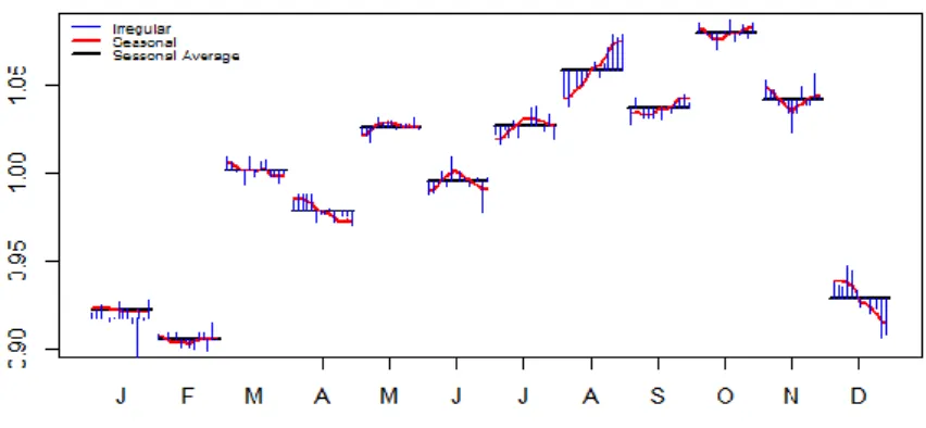
Lastly, the last two graphs to be explored by the application are related to seasonal factors and the seasonally adjusted time series. The former is useful in the assessment of the seasonal factors evolution over time, and is handled by the function monthplot() already used in the section 3.2, during the graph analysis. In the Fig. 4, obtained by the following codes, besides observing seasonal factors evolution, it is possible to watch the SI series (seasonal and irregular components, aggregated) behavior, which tends to follow the seasonal component, leading to the conclusion that the model decomposition was adequately estimated. In the Fig. 5, the seasonally adjusted industrial production graph is displayed, pointing to a worrisome decay in industrial activity since 2013.
> monthplot(seas_adjust2, col.base = 1) > plot(seas_adjust2)
Figure 4: Seasonal and irregular components, monthly
Figure 5: Industrial Production, seasonally adjusted
4. Final Remarks
In this article we have learnt what is seasonal adjustment and why this is important. We have seen that there are many ways to extract the seasonal term, although we have focused on just one: the seasonal adjustment program X-13ARIMA-SEATS from the US Census Bureau. We have learnt the steps to run the X13 using R and the methods to evaluate the seasonal adjustment performance taking into account a lot of diagnoses. In addition, we have also seen the usefulness of the pre-adjustment phase in X13, which allowed us to insert other variables, improving the diagnosis assessment.
Although we have shown many methodologies to evaluate the quality of the seasonal adjustment, it is important to be clear that all the methods have limitations and, if possible, the reader should consult other sources of information.
References
ADLER, J. (2009). R in a Nutshell. Sebastopol, CA: O'Reilly.
BRAUN, W. J., & MURDOCH, D. J. (2008). A First Course in Statistical Programming with R. Cambridge
University Press.
DALGAARD, P. (2008). Introductory Statistics with R. LLC, New York: Springer Science + Business Media.
EUROSTAT. (2016). Outliers. Tratto da E-learning Courses - Seasonal Adjustment: https://ec.europa.eu/eurostat/sa-elearning/outliers
FERREIRA, P. C., MATTOS, D. M., OLIVEIRA, I. C., LIMA, L. F., & DUCA, V. E. (2016). Análise de
Séries Temporais usando o R - um curso introdutório. Rio de Janeiro: Working Book.
FINDLEY, D. F., MONSELL, B. C., BELL, W. R., OTTO, M. C., & CHEN, B. C. (1998). New Capabilities and Methods of the X-12-ARIMA Seasonal Adjustment Program (with discussion). Journal of Business
and Economic Statistics, 12.
GÓMEZ, V., & MARAVALL, A. (1996). Programs TRAMO (Time series Regression with Arima noise, Missingo observations, and Outliers) and SEATS (Signal Extraction in Arima Time Series. Instructions for the User. Working Paper, Banco de España.
HODGESS, E. M. (2004). A Computer Evolution in Teaching Undergraduate Time Series. Journal of
Statistics Education.
IBGE. (2016). Pesquisa Industrial Mensal Produção Física - Brasil. Tratto da Instituto Brasileiro de Geografia e Estatística: http://ibge.gov.br/home/estatistica/indicadores/industria/pimpf/br/default.shtm INSTITUTO DE PESQUISA ECONÔMICA APLICADA. (2016). ipeadata. Tratto da Ipea Data: http://www.ipeadata.gov.br/
R CORE TEAM. (2015). An Introduction to R. Tratto da The Comprehensive R Archive Network: https://cran.r-project.org/doc/manuals/r-release/R-intro.pdf
R CORE TEAM. (2016). The R Project for Statistical Computing. Tratto da https://www.r-project.org/ SAX, C. (2016). Github Christoph Sax. Tratto da Github: https://github.com/christophsax
UNITED STATES CENSUS BUREAU. (2015). Historical Papers Concerning X-11 and Seasonal
Adjustment. Tratto da X-13ARIMA-SEATS Seasonal Adjustment Program: https://www.census.gov/srd/www/sapaper/historicpapers.html
UNITED STATES CENSUS BUREAU. (2016). X-13ARIMA-SEATS Reference Manual Acessible HTML Output. United States Census Bureau. Tratto da https://www.census.gov/ts/x13as/docX13AS.pdf UNITED STATES CENSUS BUREAU. (2016). X-13ARIMA-SEATS Seasonal Adjustment Program. Tratto da United States Census Bureau: https://www.census.gov/srd/www/x13as/