Martin Damyanov Aleksandrov
Master ThesisHeuristics and Policies
for
Online Pickup and Delivery Problems
Orientador : Pedro Barahona, Professor, CENTRIA, FCT, UNL, Lisbon, Portugal
Co-orientadores : Philip Kilby, Researcher, NICTA, Canberra, Australia Toby Walsh, Group Leader, NICTA, Sydney, Australia
President: José Júlio Alves Alferes
Main referee: Paula Alexandra da Costa Amaral
Heuristics and Policies for Online Pickup and
Delivery Problems
Martin Damyanov Aleksandrov
Department of Informatics, Faculty of Sciences and Technology, Univesidade Nova de Lisboa
Advisor : Prof. Pedro Barahona, CENTRIA, UNL, Lisbon, Portugal
co-Advisor 1 : Dr. Philip Kilby, NICTA, Canberra, Australia co-Advisor 2 : Prof. Toby Walsh, NICTA, Sydney, Australia
Submission date : 15 October 2012
Declarations
I, Martin Damyanov Aleksandrov, certify that this master thesis has been written entirely by me, that is a record of work carried out by me, it has not been submitted in any pre-vious higher degree application and it will not be submitted in any future higher degree application.
I, Martin Damyanov Aleksandrov below referred to asthe Student, certify that this piece of work has been conducted in both the Universidade Nova de Lisboa, Portugal, below re-ferred to asthe Institution 1, between February 2012 and October 2012, and the National Information and Communications Technology Research Center of Excellence, NICTA, Aus-tralia, below referred to as the Institution 2, between October 2011 and January 2012. Attention has been taken with respect to both the study and graduate regulations in the Institution 1 and the working regulations imposed bythe Institution 2 as follows:
1. According to the common reguirements for obtaining a higher-education degree, posted bythe Institution 1, this work is submitted to and public available at the Depart-ment of Informatics, Faculty of Sciences and Technology, which is part ofthe Institution 1.
2. According to the conditions of the Visiting Researcher Agreement contract between
the Institution 2andthe Student, started at 1 October 2011 and finished at 18 January 2012, the Intellectual Property created during the course of this Agreement is property of
the Institution 2.
Date : Signature of the Student :
I, Pedro Barahona, hereby certify that the Student has fulfilled the conditions of the regulations appropriate for the degree of European Master in Computational Logic in the Institution 1 and that the Student is qualified to submit the thesis in application for that degree.
Date : Signature of the advisor :
I, Philip Kilby, hereby certify that the Studenthas fulfilled the conditions of the regula-tions mentioned in the Visting Researcher Agreement contract and that the Student is qualified to submit the thesis in application for that degree.
Date : Signature of the co-advisor :
Access to Printed copy of the thesis through the University Nova de Lisboa.
Date : Signature of the Student :
Preface
This Master thesis entitled”Heuristics and Policies for Online Pickup and Delivery Prob-lems”has been prepared by Martin Damyanov Aleksandrov during the period October 2011 to October 2012 at the National ICT Australia and at the Universidade Nova de Lisboa. Martin Damyanov Aleksandrov visited both places under the common study and mobility regulations of the European Master Program in Computational Logic.
The thesis work was partially supported by the National ICT Australia according to the Visitor Research Agreement contract between NICTA and Martin Damyanov Aleksandrov. The subject of the thesis is to develop new online dynamic algorithms for dispatching the fleet of vehicles for a well-known subclass of Vehicle Routing Problems, viz. Pickup and Delivery Problems, and to extend the current research in this area by possibly contributing to some basic research problems in intelligent transport systems with potential application to areas like traffic control, vehicle routing and logistics. It is motivated by a problem arised in an Australian courier firm and it aims to achieve and to satisfy their necessities as much as possible.
Next, I would like to thank my thesis advisor, Pedro Barahona, who is a professor at Uni-versidade Nova de Lisboa for his support and interest throughout this project. I have now served as Pedro’s master student during the last year and I have enjoyed our collaboration together.
I would like to thank professor Toby Walsh and doctor Philip Kilby, who are research leaders at the NICTA’s Neville Roach and Canberra laboratories, respectively. They were support-ing me dursupport-ing the whole time by givsupport-ing usefull pieces of advice, opinions and comments on the theoretical and practical aspects of this thesis.
In addition, I wish to specially thank doctor Philip Kilby for providing me technical infor-mation about the state-of-the-art Vehicle Routing Solver, Indigo 2.0, which is implemented by him and it is a property of NICTA. I really appreciate his efforts and usefull pieces of advice during the last one year.
I would like also to express thanks to Menkes van den Briel, who is an operational research professional in the optimization group at NICTA. Our discussions significantly contributed for better understanding the addressed problem.
Lastly, as a master student in such an European program I spent most of my time travelling around the world. During all this experience my family, Damyan, Svetla and Iliyan, and my friends were my moral support and I wish to thank them for encouraging me.
Abstract
In the last few decades, increased attention has been dedicated to a specific subclass of Vehicle Routing Problems due to its significant importance in several transportation areas such as taxi companies, courier companies, transportation of people, organ transportation, etc. These problems are characterized by their dynamicity as the demands are, in general, unknown in advance and the corresponding locations are paired. This thesis addresses a version of such Dynamic Pickup and Delivery Problems, motivated by a problem arisen in an Australian courier company, which operates in Sydney, Melbourne and Brisbane, where almost every day more than a thousand transportation orders arrive and need to be accommodated. The firm has a fleet of almost two hundred vehicles of various types, mostly operating within the city areas. Thus, whenever new orders arrive at the system the dispatchers face a complex decision regarding the allocation of the new customers within the distribution routes (already existing or new) taking into account a complex multi-level objective function.
Resumo
Nas ´ultimas d´ecadas, tem sido dedicada uma crescente aten¸c˜ao a uma subclasse espec´ıfica de problemas de roteamento de ve´ıculos, devido `a sua importˆancia significativa em diver-sas ´areas de transporte, tais como empresas de t´axis, empresas de courier, transporte de pessoas, transporte de ´org˜aos, etc. Estes problemas s˜ao caracterizados por sua dinˆamica, j´a que os pedidos envolvendo pares de localiza¸c˜oes s˜ao, em geral, desconhecidos com an-tecedˆencia. Esta tese trata de uma vers˜ao de Problema de Recolha e Entrega Dinˆamico, motivado por um problema surgido numa empresa de entregas australiana, que atua em Sydney, Melbourne e Brisbane, e em que todos os dias s˜ao feitos mais de mil pedidos de transporte de entregas. A empresa tem uma frota de quase 200 ve´ıculos de v´arios tipos, e opera principalmente dentro das ´areas urbanas. Sempre que um novo pedido de entrega chega ao sistema, os despachantes enfrentam uma decis˜ao complexa quanto `a aloca¸c˜ao dos novos pedidos dentro das rotas de distribui¸c˜ao (j´a existentes ou novas), tendo em conta uma fun¸c˜ao complexa fun¸c˜ao multi-objetivo.
List of Abbreviations
1. BAL - Balanced Heuristic.
2. CDVRP - The Capacitated Dynamic Vehicle Routing Problem.
3. CVRP - The Capacitated Vehicle Routing Problem.
4. CUR - Current Orders Heuristic.
5. DARP - The Dial-a-Ride Problem.
6. DPDP - The Dynamic Pickup and Delivery Problem.
7. DPDPTW - The Dynamic Pickup and Delivery Problem with Time Windows.
8. dDVRP - The Delivery Dynamic Vehicle Routing Problem.
9. DVRP - The Dynamic Vehicle Routing Problem.
10. DVRPTW - The Dynamic Vehicle Routing Problem with Time Windows.
11. GEO - Geographical Closeness Heuristic.
12. GIS - Graphical Information Systems.
13. IMM - Immediate Cost Heuristic.
14. MAV - Minimize Vehicles Heuristic.
15. MIN - Minimum Cost Heuristic.
16. ML - Machine Learning.
17. NN - Neural Network.
18. ODPDP - The Online Dynamic Pickup and Delivery Problem.
19. ODPDPTW - The Online Dynamic Pickup and Delivery Problem with Time Win-dows.
21. PDP - The Pickup and Delivery Problem.
22. PDPTW - The Pickup and Delivery Problem with Time Windows.
23. PDTSP - The Pickup and Delivery Travelling Salesman Problem.
24. pDVRP - The Pickup Dynamic Vehicle Routing Problem.
25. RAND - Random Heuristic.
26. RL - Reinforcement Learning.
27. SHIFT - Shift Profitability Heuristic.
28. STDPDP - The Stochastic and Dynamic Pickup and Delivery Problem.
29. STDVRP - The Stochastic and Dynamic Vehicle Routing Problem.
30. STVRP - The Stochastic Vehicle Routing Problem.
31. SVRP - The Static Vehicle Routing Problem.
32. TSP - The Traveling Salesman Problem.
33. UDVRP - The Uncapacitated Dynamic Vehicle Routing Problem.
List of Tables
1.1 Sydney fleet characteristics. . . 5
1.2 Bonds standart services. . . 5
1.3 Bonds extra services. . . 6
2.1 VRP constraints. . . 21
2.2 Paired and time window constraints. . . 22
2.3 Time slices scenarios. . . 24
3.1 Route constraints : regarding the arrival moment. . . 32
3.2 Route constraints : regarding the new order capacities. . . 32
3.3 Minimum Cost constraints. . . 35
3.4 Balanced constraints. . . 40
3.5 Current Orders constraints. . . 42
3.6 Shift Profitability constraints. . . 43
3.7 Geographical Closeness constraints. . . 45
3.8 Minimize Vehicles constraints. . . 46
3.9 Immediate Cost constraints. . . 47
3.10 Weaken constraints. . . 48
3.11 Worst-case complexity assesments. . . 50
4.1 Real and seeming order statistics. . . 57
4.2 Once-a-day pooling strategy : cost statistics. . . 67
4.3 Once-a-day pooling strategy : time performance. . . 68
4.4 Once-a-day pooling strategy : global valuation statistics. . . 69
4.5 Time-zones pooling strategy : global valuation statistics. . . 69
4.6 Fixed-time-span pooling strategy : global valuation statistics. . . 69
4.7 Time-zones pooling strategy : global vs. local statistics. . . 71
4.8 Fixed-time-span pooling strategy : global vs. local statistics. . . 71
5.1 Demand features. . . 76
List of Figures
1.1 The distribution of the arriving orders within a single weekday. . . 3
1.2 A specification of Vehicle Routing Problems. . . 11
2.1 Non-homogenous and periodic counting process. . . 25
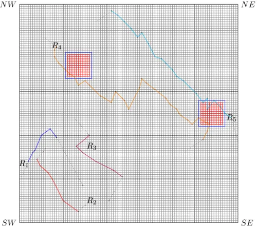
3.1 Rasterized area of Sydney. . . 44
4.1 Datasets. . . 53
4.2 Order arrival distributions. . . 53
4.3 Regression matrix. . . 55
4.4 Arrivals and weight distributions. . . 56
4.5 Comparison of the original and the generated datasets. . . 57
4.6 Evaluation procedure. . . 59
5.1 Neural network general structure. . . 75
5.2 Recommendation system scheme. . . 77
5.3 Global learning features. . . 78
5.4 Global and local learning features. . . 79
5.5 Policy comparison in oncepooling strategy. . . 81
5.6 Fleet management under πP G policy. . . 82
Contents
1 Introduction 1
1.1 Motivation . . . 2
1.1.1 Fleet and service description . . . 4
1.1.2 Objectives . . . 6
1.1.3 Summary of our problem as ODPDP . . . 7
1.2 History Notes . . . 8
1.3 Specification of VRPs . . . 10
1.4 The Vehicle Routing Solver Indigo . . . 11
1.5 Thesis contributions . . . 13
1.6 Thesis Structure . . . 14
2 A Framework for DPDP 15 2.1 The Problem Formulation . . . 16
2.2 The Basic VRP . . . 20
2.3 Paired Customers and Time Windows . . . 22
2.4 Switching to a Dynamic Setting . . . 23
2.4.1 Time slices . . . 24
2.4.2 Prediction model . . . 24
2.5 Objective Function . . . 25
2.6 NP-hardness . . . 28
3 Simple Dispatch Heuristics 29 3.1 General Assumptions . . . 30
3.1.1 Possible routes . . . 32
3.1.2 Capacity constraints . . . 32
3.1.3 Additional travel costs . . . 33
3.1.4 Time window urgency . . . 33
3.1.5 Distance measures . . . 34
3.2 Heuristics . . . 35
3.2.1 Minimum cost heuristic . . . 35
3.2.2 Balanced heuristic . . . 40
3.2.3 Current orders heuristic . . . 41
3.2.4 Shift profitability heuristic . . . 42
3.2.5 Geographical closeness heuristic . . . 44
3.2.7 Immediate cost heuristic . . . 47
3.2.8 Random heuristic . . . 48
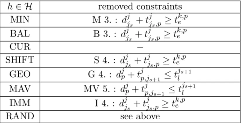
3.2.9 Weaken heuristic constraints . . . 48
3.3 Summary . . . 49
4 Heuristic Experiments 51 4.1 General Assumptions . . . 52
4.2 Benchmark Datasets . . . 52
4.2.1 Original Dataset . . . 52
4.2.2 Arrival distributions . . . 53
4.2.3 Regression analyses . . . 54
4.2.4 Predictor distributions . . . 55
4.2.5 Generated datasets . . . 56
4.3 An Experimental Framework . . . 58
4.3.1 Initial schedule . . . 58
4.3.2 Suboptimal schedule . . . 58
4.3.3 Evaluation procedure . . . 59
4.3.4 Request sequences . . . 60
4.3.5 Solutions and partial solutions . . . 60
4.3.6 Heuristic correctness . . . 62
4.4 Experimental Results . . . 63
4.4.1 Once-a-day strategy . . . 64
4.4.2 Time-zones strategy . . . 64
4.4.3 Fixed-time-span strategy . . . 65
4.4.4 Cost . . . 66
4.4.5 Time performance . . . 67
4.4.6 Correctness . . . 68
4.4.7 Global vs. local correctness . . . 70
4.5 Summary . . . 72
5 Learning Experiments 73 5.1 Machine Learning . . . 73
5.2 Neural Network . . . 74
5.3 Features, Datasets and System Scheme . . . 76
5.4 Dispatch Policies . . . 79
5.4.1 PolicyMaxSumPG . . . 79
5.4.2 PolicyMinSumPG . . . 80
5.4.3 PolicyMaxSumPLG . . . 80
5.4.4 PolicyMinSumPLG . . . 80
5.5 Experimental Results . . . 80
6 Future Perspective 86
6.1 Cross-utilization . . . 87
6.2 Traffic Congestion . . . 88
6.3 Hyper-heuristics . . . 88
6.4 Channel fleet management . . . 88
A Appendix References 90
Chapter 1
Introduction
Introduction is a new beginning. by Martin Aleksandrov
The chapter starts with the presentation of the motivational background behind our work by describing the problem source and its characteristics. We map the task in our attention into a problem of the well-known subclass of Vehicle Routing Problems (VRPs), namely Pickup and Delivery Problems (PDPs). As we deal with a courier company, where the new demands arrive dynamically, it would be beneficial to take into consideration their dynam-icity as well as to consider a prediction model of these demands, which tells us when and where a new errand would occur with some degree of certainty.
We bring the reader closer to the class of VRPs by surveying some of the relevant literature sources and by discussing some of the efforts put in such problems. The history notes do not give a total overview of such problems but we attemp to track the research line in this area along the years and give an additional motivation to our project. In parallel, we highlight the features of our work in order to support it with a more clear distinction from the previous work.
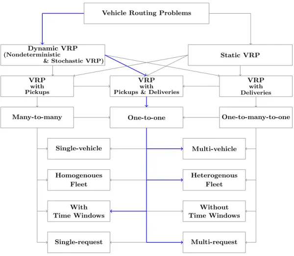
The next section presents a specification of the VRPs. In the past many people have spec-ified these problems and we do not argue that our criterion is a total or an unique one, rather we present it to narrow the attention of the reader to the task we deal with. We capture our characterization of the VRPs with a figure, depicting the relations between the different subclasses and underlining the assumptions made within each one of them.
1.1
Motivation
A local courier firm has approached NICTA about providing a decision support tool to schedule their pick-up and deliveries. Bonds Express is a part of Bonds Transport Group, which has been established in 1966 and has recently grown to become a specialist multidis-cipline, Australian transport and 3PL provider. It is privately owned and it is dedicated to providing a total quality transport solution to its customers. It operates fast, secure and re-liable express courier and taxi-truck services mostly within the areas of Sydney, Melbourne and Brisbane. Offering a full range of services, Bonds has the ability to meet standart and urgent delivery needs. They also offer highly competative rates for interstate and interna-tional deliveries1.
Next, we describe the scope of the problem arised in Bonds Express Couriers. The dis-patchers in the company control six channels of information flow between the customers, requesting services, and the drivers executing these services. Each dispatcher manages one channel, which does not correspond to a region, rather to a range of vehicle types. Cur-rently, the dispatchers estimate themselves the most probable service time per job. The role of the dispatchers is of essential importance as we can view them as the distribution points in such information flows. At the same time they obey certain constraints related to their working conditions, namely they have a limited scheduling horizon and they cannot exchange information between each other. The drivers can refuse to do an assigned job and they are very selective and picky about the tasks to be performed. Currently, the order of the requests to be serviced is decided by the drivers, which means they participate in constructing their own route. The dispatchers wish to have a higher control on this or-der and to navigate the drivers towards their next destinations more precisely and routinely.
The information about vehicle locations arrive at the center dispatching unit via GPS ev-ery 3 minutes. The other direction of communication is realized via mobile text messages, which can be ambigious. Therefore, the dispatchers wish to have an improved and frequent communication with the drivers. The company has a policy of accepting all incoming job requests, even though they know they might not be able to satisfy the customer on-time requirements. In this case, the penalty for arriving too late is reflected in the profit for making the particular job. They pay the driver from the moment he picks up the first order till the moment they drop off the last one. They must pay the minimum hourly rate to the driver and keep the right to send him back home at any time. Once a driver is sent home he is no more available to the dispatchers on that day.
The fleet obeys specific limitations not only with respect to the physical characteristics of its vehicles, but also with respect to the driver contracts. According to the current work-ing conditions, drivers are allowed to work a maximum of 8 hours per day. If this time is exceeded some extra regulations are in force, which are not within our scope. Thus, each vehicle has a fixed time working horizon. In the next section, we present additional informa-tion about the fleet characteristics, i.e. type, commodities, average velocity per kilometre and an estimate of the average running cost.
1
The demands themselves must obey several restrictions. They should be serviced within limited response time, which depends on the customer as well as on the type of the chosen service. Recall, that our orders are paired and composed of a pick-up and delivery requests. Thus, a natural constraint is having the pick-up location to precede the delivery one. Be-sides the geographical and the time preference data attached to all the incoming requests, they also include information about their commodity characteristics. In practice, this would allow us to build loading and unloading process specifications for each vehicle. The latter is important as it could significantly reduce the service time at a customer location and further optimize our objectives.
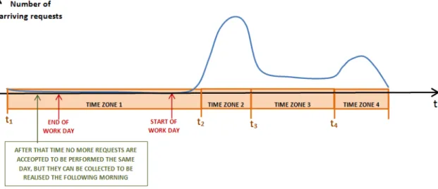
During a working day many dynamic orders arrive at the company. As expected, in the different parts of the day the order arrival frequency is different and, consequently, the total workload of the fleet would differ in these periods. Based on the distribution of the new order arrivals along the day we define four time zones. Each of them has specific characteristics such as distribution, average job commodity characteristics, most used type of vehicle within a particular zone, average travel time between clients and others, which we discuss later on. The proposed definition of time zones, which is based on the provided data is depicted in Figure 1.11, where timeti is the moment the zoneistarts. The division is as follows : Night (time zone 1), Morning pick hours (time zone 2), Day (time zone 3) andEvening pick hours(time zone 4). Figure 1.1 also shows the demand arrival rate during a single working day and it also includes the orders requested for the following days.
Figure 1.1: The distribution of the arriving orders within a single weekday.
Using this distribution we can prepare a routing and scheduling plan for the entire day, for each time zone, for a fixed time span or whenever a predefined event happens. This recalcu-lation of the plan can be made on the basis of additional information, either revealed to the
decision maker or based on historical basis. Once specified the frequency of rerouting and rescheduling of the current plan, the rules regarding the diversion of freight vehicles need to be defined. For modelling purposes, it has been assumed that the drivers can communicate with the dispatchers via communication devices installed only at client locations. As a consequence, while they are serving a client they can be informed about the changes in the routing and scheduling plan. However, each vehicle must perform the lastly assigned service.
Once a shipping parcel has been picked up, its delivery location has to be visited by the same vehicle in the same day. Hence before modifying the current sequence of clients to visit a list of compulsory delivery customers needs to be created, which cannot be shifted to any other route, but can be visited in an order different from the originally established. Although, we do not assume a possible cross-utilization amongst vehicles, in practice it might be an important issue.
1.1.1 Fleet and service description
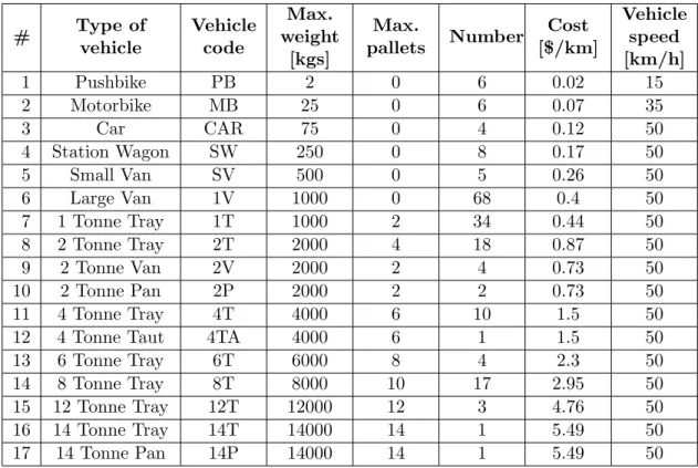
In our work we concentrate on the area around Sydney, which is lying between −33.4 and −34.4 latitude, and between 150.67 and 151.67 longitude coordinates. It covers the main metropolitan area as well as its surrounding regional centers. The core Sydney fleet is comprised of approximately 200 vehicles that range from CBD bicycles to vans and flat-tops to 14 tonne trucks and semi-trailers. We summarize the types of vehicles operating within the Sydney urban network in the Table 1.1 1. There are 17 types of vehicles, each
one described with the following features :
• vehicle type
• vehicle code
• maximum number of palletsa type is able to accommodate
• maximumload a type is able to accommodate
• numberof available vehicles of the given type
• estimate of the average cost per kilometer the company pays to have a vehicle of that type on the road
• average velocity of a vehicle
The cost was estimated taking into account the type of vehicle, its average gas and/or oil consumption per a hundred kilometres, the additional expenses when a vehicle is full and the average gas price within the Sydney area for the months between April and June, 2012
2. The velocity considered is according to the urban city speed regulations with respect to
the vehicle type, assumed an area without traffic congestion.
1According to the NICTA internal report from June 30, 2011.
# Type of vehicle
Vehicle code
Max. weight
[kgs]
Max.
pallets Number
Cost [$/km]
Vehicle speed [km/h]
1 Pushbike PB 2 0 6 0.02 15
2 Motorbike MB 25 0 6 0.07 35
3 Car CAR 75 0 4 0.12 50
4 Station Wagon SW 250 0 8 0.17 50
5 Small Van SV 500 0 5 0.26 50
6 Large Van 1V 1000 0 68 0.4 50
7 1 Tonne Tray 1T 1000 2 34 0.44 50
8 2 Tonne Tray 2T 2000 4 18 0.87 50
9 2 Tonne Van 2V 2000 2 4 0.73 50
10 2 Tonne Pan 2P 2000 2 2 0.73 50
11 4 Tonne Tray 4T 4000 6 10 1.5 50
12 4 Tonne Taut 4TA 4000 6 1 1.5 50
13 6 Tonne Tray 6T 6000 8 4 2.3 50
14 8 Tonne Tray 8T 8000 10 17 2.95 50
15 12 Tonne Tray 12T 12000 12 3 4.76 50
16 14 Tonne Tray 14T 14000 14 1 5.49 50
17 14 Tonne Pan 14P 14000 14 1 5.49 50
Table 1.1: Sydney fleet characteristics.
Standard Service Maximum Delivery time
Standard Courier 3 hours
Priority Courier 1 hour and 55 minutes Express Guaranteed arrangement on the phone
Table 1.2: Bonds standart services.
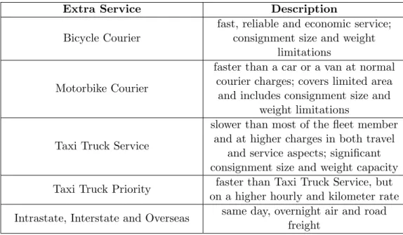
The fleet tries to satisfy each customer necessity through a variety of standard and extra services. The standard services are summarized in Table 1.2 together with the maximum delivery times within which they should be performed, and the extra services are described in Table 1.31. The actual average delivery times are significantly less than the maximum
quoted, although these are subject to traffic and weather conditions. Extra time of approxi-mately 25% should be allowed for meeting deadlines of deliveries of more than 30 kilometres driving distance and to destinations outside the metropolitan area2. Recall, that the
con-ditions of the type of service are discussed with the customer when the demand is being requested and they are incorporated in his time preferences.
1According to the NICTA internal report from June 30, 2011.
Extra Service Description
Bicycle Courier
fast, reliable and economic service; consignment size and weight
limitations
Motorbike Courier
faster than a car or a van at normal courier charges; covers limited area
and includes consignment size and weight limitations
Taxi Truck Service
slower than most of the fleet member and at higher charges in both travel
and service aspects; significant consignment size and weight capacity
Taxi Truck Priority faster than Taxi Truck Service, but on a higher hourly and kilometer rate
Intrastate, Interstate and Overseas same day, overnight air and road freight
Table 1.3: Bonds extra services.
1.1.2 Objectives
Here we list the objectives the company is willing to achieve. As this master thesis is a part of a bigger project, whose final goal is to deliver an end-user product to the company, i.e. a decision supporting tool, we concentrate on those aims more relevant to our problem.
1. The minimum number of requests assigned to a vehicle type in order to ensure prof-itability for the shift.
2. The time of active performance of a vehicle type, i.e. without waiting times.
3. The average number of requests per driver per vehicle type.
4. The average schedule duration per driver per vehicle type.
5. The degree of dynamism of the addressed problem.
6. The maximization of simultaneous utilisation of vehicles for multiple deliveries.
7. The improvement of the overall fleet utilization.
8. The capacity of any vehicle that should not be exceeded at any time.
9. The satisfaction of the customers, which is improved by ensuring more on-time ser-vices.
11. The number of contracted drivers in relation with the jobs performed for a single day. The objective is to minimize the former and to maximize the latter.
12. The number of drivers to be contracted at the beginning of the working day and the number of those sent home along the day.
13. The order, in which a driver visits the clients.
14. The final cost to be minimized.
1.1.3 Summary of our problem as ODPDP
In this subsection we extract all relevant information from the informal specification given above in order to concentrate on the problem in hands. We restrict the problem to the Sydney fleet of the company and services only within the metropolitan area and its sur-ronding regional centers. We consider a heterogenous fleet of 192 vehicles, each with a type, capacities, running cost and running velocity described in Table 1.1. Each vehicle has a home location which is where the day starts and ends. Once a vehicle leaves its depot, the firm pays a cost per hour until the vehicle returns at the end of its shift. We consider a shift length of minimum 1 and maximum 8 hours per day. Also each vehicle type has a given capacity in terms of weight and number of pallets. There are hard constraints on the total weight and the total number of pallets that can be carried at any one time.
The problem is dynamic as the orders can arrive at any time. Each order is described by an order id, order arrival time, order weight, order pallets, pick-up location, earliest pick-up time, latest pick-up time, delivery location, and latest delivery time. The earliest pick-up time is a hard constraint as the package is assumed not to be ready before this time. We may require vehicles to wait at a location till the earliest pick-up time constraint is sat-isfied. The latest pick-up and delivery times are soft constraints and there are piecewise linear penalty terms in the objective for violating these constraints. There are service times for each location to account the time needed to collect or deliver the requested parcel. Due to the lack of more precise information about the fleet and order commodity dimensions we could not build loading and unloading specifications for the vehicle types, and assume 3 minutes of service time for goods less that 250 kilograms and 10 minutes 1, otherwise. The pick-up and delivery times are defined by the customer. They express his preferences and can be arranged during the booking time. The type of service needed is also taken into account when these preferences are discussed. In addition, we suppose orders are scheduled within a single day, assuming that some of them have been requested some days before. In reality, we may hold requests at the end of the day for the next morning, afternoon, evening or even for several subsequent days.
Importantly, the routing is supposed to be online. Whilst we may have a tentative schedule for all current orders, we only commit to a pick-up or delivery when the previous demand has been executed. A vehicle can be diverted at a client location, but not along its way between any two consecutive visits. The driver may consult with a dispatcher about his
next destination via PDA device. Finally, we do not allow any load to be stored at any of the depot, customer or intermediate locations. In practice, a vehicle could deliver a package to some place, called store, where another or even the same vehicle will arrive later and collect the particular good. The last would be an interesting extension to our work, but since our focus is centered on learning dispatch decisions we do not consider this issue.
1.2
History Notes
A Vehicle Routing Problem (VRP) can be defined as a problem of finding the optimal routes of delivery or collection from one or several depots to a number of cities or customers, while satisfying some constraints. Collection of household waste, gasoline delivery trucks, goods distribution, snowplough and mail delivery are the most used applications of the VRP. The VRP plays a vital role in distribution and logistics. Huge research efforts have been de-voted to studying the VRP since 1954 when Dantzig and Ramser [17] have described the problem as a generalised problem of Travelling Salesman Problem (TPS). Since this point onwards a tremendous amount of research work has been concentrated on the comparison between practically expensive exact methods and heuristic approaches. Some of the work on this subject after the eighties are Christofides et al., 1981 [12], who used spanning tree and shortest path relaxations to solve a number of instances derived from the literature. Desrochers, Lenstra and Savelsbergh in 1990 [18] (Laporte, 1992 [42]) surveyed main exact and approximate algorithms developed for a VRP, at a level appropriate for a first graduate course in combinatorial optimization. Later on Baldacci et al. in 2008 [5] introduced an exact algorithm for the capacitated version of a VRP (CVRP) based on the set partitioning formulation and additional cuts that correspond to capacity and clique inequalities in the VRP graph. Baldacci also discussed some recent advances the same year (2008) in [4]. Apart from the classical formulation and its variants also many efforts have been made in modelling specific optimization problems by means of VRP. For instance, Dong et al. 2011 described a variant of VRP in Flight Ticket Sales Companies for the service of free pickup and delivery of airline passengers to the airport (see [20]).
2004, [41]). Also the limited knowledge of the incoming demands motivated people to take a close look over the heuristics for Stochastic VRPs (STVRP). Swihart and Papastavrou [55], 1999, considered demands arriving according to a Poisson process. In 2006, Ichoua ([32]) exploited a strategy based on a probabilistic knowledge about future requests in or-der to predict where such a stochastic event would occur. Such approaches usually improve the fleet management. Later on Hvattum et al. [31], 2007, implemented a Branch-and-Regret heuristic for Stochastic and Dynamic VRP (STDVRPs). Several other practically important variants such as DVRP with Time Windows (DVRPTW), DVRP with Pick-Ups (pDVRP), DVRP with Deliveries (dDVRP), DVRP with Pick-Ups and Deliveries (DPDP, Parragh et al. 2008 [50]) and Capacitated DVRP (CDVRP, Kopmanz et al. 2001 [40], Ganapathy et al. 2009 [23], Chandran and Raghavan, 2008 [11]) as well as Uncapacitated DVRP (Angelelli et al. 2007 [1]) have also been investigated thoroughly.
The class closer to this thesis is a variant of DPDP. Its instances are characterized with additional considerations regarding the demands, e.g. the deliveries are paired and they must be executed in a particular order (i.e. the pickup location to be visited before the delivery one). In other words, objects or people have to be transported between an origin and a destination. Moreover, issues related to the order arrival dynamicity and to antici-pating future demands should be taken into account, and therefore we consider Stochastic and Dynamic PDP (STDPDP). Furthermore, the class of PDPs can be classified into three different groups. The first group consists of many-to-many problems, in which any vertex can serve as a source or as a destination for any commodity. An example of a many-to-many problem is the Swapping Problem (Anily and Hassin, 1992 [2]). In this problem, every vertex may initially contain an object of a known type of commodity as well as a desired type of commodity. The problem consists of constructing a route performing the pickups and deliveries of the objects in such a way that at the end of the route, every vertex possesses an object of the desired type of commodity. Problems in the second group are called one-to-many-to-oneproblems. In these problems commodities are initially available at the depot and are destined to the customer vertices; in addition, commodities available at the customers are destined to the depot. Finally, in one-to-oneproblems, each commodity (which can be seen as a request) has a given origin and a given destination. Problems of this type arise, for example, in courier operations and door-to-door transportation services. Thus, our problem can be classified as one-to-one PDP. In addition, we assume customer preferences on time windows (PDPTW, Mini´c, 1998 [47] and DPDPTW, Mitrovi´c-Mini´c et al., 2004 [43]) and stochasticity (STDPDP, Chun-Mei, 2011, [13]).
Irnich studied the multi-depot PDP with a single hub and heterogenous fleet. He focused on problems where all possible routes can easily be enumerated, i.e. the problem primar-ily considers the assignment of transportation requests to routes. The hub serves as a consolidation point which often assumes short routes between it and the locations in the transportation network, i.e. involve only one or very few customers. The rationale for this one is in the narrow time windows as well as in the high quantities, which make it pos-sible to fully load a vehicle at one customer. Recall, the Bonds Express Couriers has at its disposal a heterogenous fleet, whose members have their own depot. Consequently, the variant we consider is a multi-depot OSDPDPTW. In addition to the quantitave and type description of the fleet a significant attention is devoted to the commodity dimensions of the fleet members. For example, Hern´andez-P´erez and Salazar-Gonz´alez in 2005 ([28]) stud-ied the multi-commodity version of PDTSP, while in 2011 ([52]) Psaraftis explored exactly dynamic programming solutions for the multi-commodity PDP when one or two vehicles are available. In this thesis we assume a fleet, which has several commodity dimensions. In our case these are the number of pallets and the weight a particular order is composed of.
We are interested specifically in learning dispatch policies to control the fleet of vehicles online, rather than using an offline approach. We are not aware of much research in this precise setting. Inspired by this and the real case-study arisen in the courier company we designed a recommendation system, which applies dispatch rules whenever a new errand arrives taking into account the current parameters of the overall fleet. The decisions made by the system also take into account the possibility of unreserved demands to occur. There are several attempts to dispatch the fleet of vehicles, which we report next. For instance, Cort´es et al. (2008, [15]) applied a hybrid-predictive control for fixed-fleet size DPDPs including traffic congestion, incorporating future information regarding unknown demands and expected traffic conditions. Also Gendreau et al. (2006, [24]) proposed neighborhood search heuristics to optimize the planned routes of vehicles in a context where new re-quests, with a pick-up and a delivery location, occur in real-time. Their study is based on ejection chains technique and, furthermore, they investigate the impact of a master-slave parallelization scheme on the optimization process. Two years later, in 2009, Beham et al. ([6]) considered agent-based simulation of dispatching rules in DPDP. This work treats the topic of solving dial-a-ride problems. A simulation model is introduced that describes how an agent is able to satisfy the transportation requests using a complex dispatching rule, which is optimized by metaheuristic approaches. The authors are using fitness function in order to evaluate the quality of the agent state.
1.3
Specification of VRPs
previously-known customer. Another issue we omitted is related with the traffic congestion. On could argue that the traffic is important feature in areas such as courier, cap companies, etc. and a problem instance could be classified with respect to the intensity of the traffic conditions. To emphasize the instance we deal with, we draw a blue line starting from the root, passing through the nodes matching our assumptions, and it ends into several nodes describing some of the general fleet, customer and dynamic features taken into account during modelling the real case-study.
Vehicle Routing Problems
Static VRP Dynamic VRP
(Nondeterministic
& Stochastic VRP)
VRP
with Pickups
VRP
with Deliveries
VRP
with
Pickups & Deliveries
Many-to-many One-to-one One-to-many-to-one
Single-vehicle Multi-vehicle
Homogenoues Fleet
Heterogenous Fleet
With Time Windows
Without Time Windows
Single-request Multi-request
Figure 1.2: A specification of Vehicle Routing Problems.
1.4
The Vehicle Routing Solver Indigo
a VRP instance. The process of creating such a schedule, which helps in managing the fleet of vehicles, is divided into two main phases. During the first, the system constructs visiting assignments to each vehicle subject to the following requirements :
1. It returns ordered routes.
2. The objective could be specified in terms of distance, time or cost measures.
3. It allows arbitrary customer requests, i.e. pickups and deliveries.
4. A single time window for each customer location.
5. Vehicle limits, i.e. maximal capacities.
6. Vehicle availability window, i.e. the time when a particular vehicle is available. The start and end locations are arbitrary.
7. Compatibility constraints.
8. Metrics (i.e. distance, time, cost) represented as a matrix of values between any two locations.
9. Only one route per vehicle is allowed.
The usual way to construct a solution to routing problems is via insertion. That is, the representation of the emerging routes is kept internally. The system first chooses a visit to insert, then looks at all possible insertion points and when the best such point is selected, it updates the routes, and continues by considering the next visit. The insertion methods implemented are basically weighted combinations of visit characteristics such as :
1. The number of routes where the visit can be feasibly inserted into.
2. The width of the time window(s).
3. The size of the load(s).
4. The minimum insertion cost.
5. The insertion regret cost (difference between best and second-best cost).
6. The amount the insertion reduces the slack (spare time) in the best route.
Once the initial routes are built, they are subsequently improved by means of local search during the second phase of constructing the final schedules. The VRP Solver searches for a neighbour solution (defined according to one of a number of local search neighbourhoods) that is both feasible according to the basic constraints, and cost-reducing. When one is found, Indigo calculates the true cost and feasibility of a possible implementation using invariants. This is the cost which would then be used to determine whether the change is accepted. The following local search neighbourhoods are realized in Indigo :
2. Or-opt considers moving a sequence ofkconsecutive visits to another route or another part of the same route, in both forward and reverse orientations. The numberkusually is of an order between 5 and 10.
3. Large Neighbourhood Search partially deconstructs (removes visits from the solution) and then re-constructs the solution. To do the last it uses the construction methods listed above. Thus, in effect a call to the VRP Solver with a partially-constructed so-lution is made, but acceptance of the resulting soso-lution depends on the meta-heuristic being used. The designed meta-heuristics for that purpose are Hill-climbing - best first, Hill-climbing - first-found, Adaptive tabu search, Limited Discrepancy Search and Simulated Annealing.
The quality of the final schedules in terms of the specified objective depends partly on the number of the improvement iterations performed during the second implementation phase. In our work, all the solutions produced are improved under the same parameter settings, which allow us to use them as an uniform baseline during the experiments. The parameters we used to build solutions are Large Neightbourhood Search ([16]) combined with the Sim-ulated Annealing ([21]) meta-heuristic, for a total number of 10000 improvement iterations.
1.5
Thesis contributions
Here we summary the contributions we made in the field of Vehicle Routing Problems. An Australian courier company has approached NICTA to provide a decision-support tool for managing their deliveries. Motivated by this problem we concentrated on the development of a recommendation module for this tool. We first introduced a theoretical framework within which we conducted our research. Although, there are many such frameworks in the literature, we adopted one fitting best to our needs. We modelled the real case-study as an Online Stochastic and Dynamic Pickup and Delivery Problem. The latter VRP variant has been investigated thoroughly within the last years, however, not much research attention considers the exact assumptions we made.
In order to support the company workforce in dispatching the fleet we implemented eight online dispatch heuristics, which take into account the current status of the fleet together with the new demands. This set is composed of the rules Minimum Cost, Balanced,
Current Orders, Shift Profitability, Geographical Closeness, Immediate Cost,
Minimize Vehicles and Random. For each rule we presented its algorithm as well as discussed its correctness and complexity.
the results and reached the conclusion that the best profit gained with respect to the offline solution was achieved whentime-zones strategy was applied. We also reported various de-scriptive statistics for each of the scenarios.
In the last part of our work we presented the recommendation module. Under its scheme we implemented four ad-hoc policies and we discussed their performance. These are
Min-SumPG, MaxSumPG, MinSumPLG and MaxSumPLG policies some of which are
based only on global features and others take into account also local properties. We com-pared the results produced with the offline schedules for thirty days of client requests. The best performance in terms of final cost in once pooling strategy was achieved by Min-SumPLG, however, the best management in terms of used vehicles and cost was realized byMaxSumPGpolicy. Intime-zonesandfixed-time-spanall the policies performed good. However, using more vehicles is crucial in the final cost minimization (MinSumPG and
MinSumPLG). On the other hand, if one is interested in using less human resources, then pursuingMaxSumPGorMaxSumPLGcan be beneficial as they actuate relatively smaller number of vehicles and at the same time achieve good final cost values. Our online system achieved costs 34−43% above than those obtained using Indigo in theonce-setting and in thetime-zonesit even outperformed the solver for some of the time slices and policies.
1.6
Thesis Structure
Chapter 2
A Framework for DPDP
Being predictive optimizes the costs. by Martin Aleksandrov
This chapter begins with the description of the framework we used to model the addressed problem. It introduces several appropriate notions and notations (i.e. time windows,pickup and delivery route, etc.), which are relevant to our work and highlights several features of the problem in hand.
Subsequently we formulate the basic model of a VRP in terms of a linear integer program. We present the collection of constraints used and explain their semantics. Next, we in-troduce the additional requirements imposed by the fact that each call in the company contains information about two connected demands, i.e. a pick-up and a delivery requests. Precedence limitations related to these services are also considered and presented together with client preferences in terms of time windows for both subdemands.
The chapter continues with a discussion on two important questions arising in the dynamic PDPs. The first one is related to the possibility of weakening the dynamic burder implied by the multiple daily arrivals and the second one affects the subject of predicting those demands. We discuss relevant strategies such as splitting the working horizon into time slicesand using a stochastic model in order to anticipate future demands.
2.1
The Problem Formulation
Fleet In our model, we have m < ∞ vehicles with different capacity characteristics. Let we denote the set of them with V = {v1, . . . , vm}. For each vehicle vj we denote the maximum number of pallets and weight capacity withQj andUj, respectively. These values should never be exceeded. Each day vehicle vj starts and ends its shift at so-called depot
dj with no cargo loaded. We denote as D ≡ ∪mj=1dj the set of all depot locations. Lastly, each vehiclevj performs with different average velocity on the road.
Orders An orderis a demand requested to the central dispatcher unit either through a phone or an internet inquiry. Let the set of all transportation orders beO ={o1, . . . , on}. Each order oi ∈ O is composed of quantities qi and ui (number of pallets and weight, respectively). These are to be transported from an origin l1i to a destination l2i, satisfying the customers time preferences at these locations.
Requests A request is a subdemand, which contains information only about the pick-up or the delivery customer. Thus, each order oi ∈ O corresponds to two requests. By
RO ={r11, r21. . . , r1n, r2n}we denote the set of all transportation requests, whereoi= (ri1, r2i),
ri1 and ri2 being the i-th order with its corresponding pick-up and delivery requests. The commodity values are positive for a pick-up and negative for a delivery request.
Urban network LetL1≡ ∪n
i=1l1i and L2 ≡ ∪ni=1l2i be the sets of all pick-up and delivery locations, where n is the number of orders. Furthermore, let L≡L1∪L2 be the set of all the customer locations and|L|≤2∗nbe its upper bound. Thus, we have at most 2∗n+m
(customer plus depots) distinct locations and for every pair li, lj ∈ L∪D, let di,j denote the distance betweenli andlj, and tki,j the travel time between them by a vehicle vk∈V.
Time windows Each request ri ∈ RO has an associated time window, i.e. the time interval, in which service at the particular location must take place. For oi = (r1i, ri2)∈O, the time window for ri1 is denoted by [ti,e1, ti,l1] and for ri2 by [ti,e2, ti,l2]. The release time is the earliest time a request anddeadlineits latest time.
Service time Each visit to a particular location requires time for executing the services related with it, such as loading or unloading. We call this period the service time associ-ated with the considered request. This time usually depends on the vehicle performing the service and it may differ for the pick-up and the delivery services and customers, but in this thesis we assume them to be equal at both the order locations and vehicle-independent. Therefore, if oi= (ri1, ri2) is an order and each request location requiressi time units, then the service time for the whole order is 2∗si. In addition, the depots are the only locations, to which no service times are associated.
A customer requestrk
i ∈RO is thus represented by the following tuple :
where (1) ti is the arrival time of rik, (2) the second and the third components are the commoditiesqi and ui, however, they are multiplied by an addition term, which is 1 if the request is a pick-up and −1, otherwise, (3) the request time window and (4) the location where the request has been required.
The first definition below relates the vehicles in the fleetV with a set of requests, while the second generalizes that relationship for the entire fleet. Both definitions impose constraints on the vehicle management.
Definition 1 : (Vehicle Route) Let V = {v1, . . . , vm} be a vehicle fleet. Then for each
vj ∈V a pick-up and delivery routeRj ={rj1, . . . , rjnj} (PDR) is an ordered set of visits
through a subset ofRO such that :
• rj1, rjnj are associated withdj ∈D and norjm withm∈ {2, nj−1}does.
• For a given order oi ∈O both or neither r1i and ri2 belong to Rj. If both r1i and ri2 belong toRj, thenr1i is serviced beforeri2.
• The vehiclevj services each request in Rj exactly once.
• The total load of all pickups in Rj does not exceed the maximal commodity values
Qj and Uj, at any location.
• For each requestrjm∈Rj, the time window is feasible, i.e. t
jm
e ≤tjlm.
Note that the first and the last visit in a PDR (the depot) are virtual requests and can be represented, for eachdj ∈D, with the tuple <0 : 00, 0, 0, [cj ,fj], dj >, where (1) [cj, fj] is the depot shift-time window, which opens atcj and closes atfj, and (2) dj is the j−th depot location. We denote the set of these requests as RD and we call each element from ita home request.
Definition 2 : (Routing Plan) LetV ={v1, . . . , vm}be the considered fleet. Apickup and delivery routing plan(PDRP) for managing the fleetV is a set of routesR={Rj |vj ∈V} such that :
• The routeRj is a pickup and delivery route for each vehiclevj ∈V.
• The set{Rj |vj ∈V}is a partition of RO.
We thus defined the vehicle routes as disjoint sets of requests, whose union results in the entire setRO. Each of them contains information about the total load a vehicle has to carry, but they do not address timing at the locations, possible waiting times for early arrivals or delays for late arrivals. These are captured by the following definitions.
• For each Rj = {rj1, . . . , rjnj}, there is an associated itinerary Ij = {ij1, . . . , ijnj}.
Each element ijk is called the timetable associated with the request rjk or request
itinerary is defined as,
ijk =< a
j jk, w
j jk, b
j jk, sjk, e
j jk >,
whereajj
k,w
j jk,b
j
jk,sjk ande
j
jk are the arrival, waiting, starting, service and departure
times for the given request.
Similarly, to the home requests we define a timetable at each depot locationdj ∈D. That is, a tuple of the form : < cj, 0, cj, 0, pj >, where cj is the time a vehicle is available at
dj and pj is the time when it leaves that location. We call such a tuple home itineraryand the set of those we denote asID.
Definition 4 : (Routing and Scheduling Plan) A pickup and delivery routing and
scheduling plan (PDRSP) is a pair P = (R,I), where R is a routing plan and I is a scheduling plan for it.
From now on we assume that whenever we discuss a PDRSP we know its underlying set of orders. When we work with multiple sets of demands we will explicitly refer to one if needed. Our final goal is to construct such a routing and scheduling plan achieving con-venient total costs and managing the fleet in a reasonable way during that day. The next measures address the quality of a fleet schedule. We do not argue that these are all the measures for evaluting a given plan. Rather than, they were reasonably chosen represent-ing the company interests. From now on in order to avoid a possible confusion with the notations every time we need a component of a particular request rjk or an itineraryikj we will refer to it directly.
Definition 5 : (Vehicle performance) LetP = (R,I) be a PDRSP andRj ={rj1, . . . , rjnj}
be a PDR executed by a vehicle vj ∈V following timetable Ij ={ij1, . . . , ijnj}.
• Duration(j, P) =ejj
nj−1−a
j
j2 is the duration of the routeRj
• F reeP(j, l, P) = (Qj− l
X
k=1
qjk) for eachl∈ {1, . . . , nj}is the free capacity invj with
respect to the number of pallets at visitrjl
• F reeW(j, l, P) = (Uj− l
X
k=1
ujk) for eachl∈ {1, . . . , nj}is the free capacity invj with
respect to the weight at visitrjl
• ServiceT ime(j, P) = nj
X
k=1
• W aitingT ime(j, P) = nj
X
k=1
wjj
k is thewaiting timeof route Rj
• Lateness(j, P) = nj
X
k=1
ljj
k is the total lateness of route Rj, where l
j jk = b
j jk −t
k l, if
bjj
k > t
k
l or 0, otherwise, is the lateness at visitrjk by vehicle vj
• T ravelT ime(j, P) = nXj−1
k=1
tjk,k+1 is the total travel timeof route Rj
• ExecutionT ime(j, P) =T ravelT ime(j, P)+W aitingT ime(j, P)+ServiceT ime(j, P) is the total execution timeof routeRj
• U nsat(j, P) = nj
X
k=1
penalty(rjk) is the number ofunsatisfiedcustomers alongRj, where
penalty(rjk) = 1, if l
j
jk >0, and 0, otherwise
The best profit ofRj in terms of serviced clients and execution time could be achieved if we maximize nj and minimize ExecutionT ime(j, P), and Lateness(j, P) possibly satisfying all hard and soft constraints. As for each request rjk ∈ Rj, sjk is fixed at the location
lk, then ServiceT ime(j, P) will be fixed for nj requests. Moreover, under the assump-tion that the fleet of vehicles are moving with constant velocity on the road, we have that
T ravelT ime(j, P) is also fixed for a given route. Hence, for a fixed number of customers along Rj, we can minimizeExecutionT ime(j, P) only if we minimize W aitingT ime(j, P). In addition, minimizing Lateness(j, P) will maximize the customer satisfaction, i.e. max-imize the number of on-time deliveries. Despite the vehicle measures above, one is more interested in overall fleet performance or in the quality of work a particular vehicle type produces throughout the day. The former gives a possibility to evaluate the entire fleet schedule, while the latter observes more the road behaviour of a particular subset of the fleet.
Definition 6 : (Fleet performance) Let V = {v1, . . . , vm} be the fleet of vehicles,
O={o1, . . . , on}be a set of transportantion orders, andP = (R,I) a PDRSP for managing
O by V. Then we define the following features related with this plan :
• ServiceT ime(P) = m
X
j=1
Service(j, P) is theservice time of planP
• W aitingT ime(P) = m
X
j=1
W aiting(j, P) is thewaiting timeof planP
• Lateness(P) = m
X
j=1
• T ravelT ime(P) = m
X
j=1
T ravel(j, P) is the travel timeof plan P, i.e. the total travel
time of the fleet
• ExecutionT ime(P) =T ravelT ime(P) +W aitingT ime(P) +ServiceT ime(P) is the total execution timeof planP
• U nsat(P) = m
X
j=1
U nsat(j, P) is the total number ofunsatisfied customers in P
• Active(P) ={Rj |Execution(j, P)6= 0} is the set of active vehicles inP
Definition 7 : (Type performance) Let O = {o1, . . . , on} be a set of transportantion orders and V = {v1, . . . , vm} the fleet of vehicles. If T is a vehicle type, then by VT =
{vj |vj ∈V and it is of typeT} we denote the set of vehicles of type T. Furthermore, let
P = (R,I) be a PDRSP. Then the pairPT = (RT,IT) represents a PDRSP forVT, where the sets RT ={R
j |Rj ∈ R and vj ∈V is of type T} and IT ={Ij |vj is of type T} are, respectively, the routes performed only by vehicles of that type and their itineraries.
• nT = |RT|
X
j=1
(nj −2) is the total number of serviced locations by the vehicles of that
type wherenj is the number of visits inRj ∈ RT
• ActiveTR= |RT|
X
j=1
(Service(j, PT) +T ravel(j, PT)) is the time of active performance of
the vehicles from VT
• nTj = 2∗|ActivenT(PT)| is the average number of serviced orders per driver of a vehicle
from VT
• AverageDur(PT) = |RT|
X
j=1
Duration(j, PT)
|RT| is the average schedule duration per vehicle
from VT.
2.2
The Basic VRP
to RO. Lastly, the variable zijc stores the cummulative load for the commodity c∈ {q, u} carried by vehiclevj, visiting locationliof requestri ∈RO. It accepts only natural values as we consider a natural number assigned to each commodity. In each time instant this value should be less or equal than the maximum allowed for the particular commodity in vehicle
vj. As the only locations where a vehicle could change its capacities are the customer ones, which belong to its route, the value ofzc
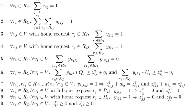
ij will increase after visiting a pick-up location and it will decrease when service at a delivery location is performed. Next, we define the VRP problem in terms of integer constraints using the variables we defined as follows:
1. ∀ri ∈RO. m
X
j=1
xij = 1
2. ∀ri ∈RO. m
X
j=1
X
rk∈RO
yikj = 1
3. ∀vj ∈V with home request rj ∈RD.
X
ri∈RO
yjij = 1
4. ∀vj ∈V with home request rj ∈RD.
X
ri∈RO
yijj = 1
5. ∀ri ∈RO.∀vj ∈V.
X
rk1∈RO
yk1ij−
X
rk2∈RO
yik2j = 0
6. ∀ri ∈RO.∀vj ∈V.
X
rk∈RO
yikj∗Qj ≥zijq +qi and
X
rk∈RO
yikj ∗Uj ≥zuij+ui
7. ∀ri1, ri2 ∈RO∪RD. ∀vj ∈V. yi1i2j = 1 ⇒ z
q
i1j+qi2 =z
q
i2j and z
u
i1j +ui2 =z
u i2j 8. ∀ri ∈RO.∀vj ∈V with home request rj ∈RD. yjij = 1 ⇒ zijq = 0 and ziju = 0 9. ∀ri ∈RO.∀vj ∈V with home request rj ∈RD. yijj = 1 ⇒ zjjq = 0 and zujj = 0 10. ∀ri ∈RO.∀vj ∈V. zijq ≥0 andziju ≥0
Table 2.1: VRP constraints.
the pick-up and the delivery locations, respectively. Next, constraints 8 and 9 impose that each vehicle depart from and arrive at its depot empty and the last constraint keeps the values of the current cummulative commodities non-negative.
2.3
Paired Customers and Time Windows
Following the basic constraints in the previous section, we introduce constraints to impose that each order is paired (comprised of pick-up and delivery requests). Hence, our locations are connected and under our assumptions such places should be visited by the same vehicle. A natural precedence constraint is presented and discussed. In addition, each request has its own time preferences, i.e. time window within which the service at a particular location should take place. The earliest such time is a hard constraint as we assume that the package is not ready before that time. Consequently, if a vehicle arrives earlier than this time, it should wait in order to start its services. The latest time for a given location is a soft constraint and it could be violated. We pay a penalty for such a delay, which is taken into account when we consider the objective function.
Next, we proceed more formally. Let oi = (r1i, ri2) ∈O be an order. Let ri1 be at location
l1i andr2i at locationl2i. In addition, let [tei,1, ti,l1] and [ti,e2, ti,l2] be the time windows related to these locations. Let the demand oi to be assigned to vehicle vj ∈V and let Ij ∈ I be its itinerary in planP = (R,I). Futhermore, let pj be the departure time for that vehicle. Thus, in addition to constraints 1. - 10., the following constraints should also be satisfied.
11. ∀oi ∈O∀vj ∈V. xi1j = 1⇔xi2j = 1 12. ∀oi ∈O∀vj ∈V. xi1j +xi2j = 2⇒djj
i1 ≤d
j ji2 13. ∀oi ∈O. ti,e1 ≤tli,1 and ti,e2 ≤ti,l2
14. ∀ri, rk∈RO. ∀vj ∈V. yikj = 1⇒djji+tji,k ≤djjk 15. ∀ri, rk∈RO. ∀vj ∈V. yikj = 1⇒djji+t
j i,k =a
j jk
16. ∀ri, rk∈RO. ∀vj ∈V. yikj = 1⇒ajji+wjji+sjji =djji 17. ∀rj ∈RD. dj1 ≥pj
Table 2.2: Paired and time window constraints.
from a location, it arrives at the next one after the required time units. We assume that the vehicle driver does not wait somewhere on his way between the two locations. The only place he is allowed to wait is at a customer location whenever he arrives earlier than the earliest time for that location. The length of the waiting time window associated with a request ri ∈ RO is wi = tie−ai if ai < tie and 0, otherwise. We assume that in the latter case, the driver starts serving the client immediately after he arrives, as expressed by constraint 16. In other words, the only time a driver spends at a customer location is equal to the service time needed for the corresponding demand. Within this time the driver could consult a dispatcher about his next destination and then to head towards it. The final condition simply says that each vehicle departs from its home location at the departure time associated with that depot.
Costraints 1-17 represent a linear integer program corresponding to the static version of our problem. This program models our problem as a PDPTW. However, the addressed problem is dynamic as the client orders arrive unpredictable. Thus, hereafter, we discuss the issues related with the dynamic PDPTW version.
2.4
Switching to a Dynamic Setting
In this section we discuss the issues related to the problem dynamics. First, we deal with the so called one-to-one PDPTW. In other words we have a fleet of vehicles that leave empty their home locations, serve a particular number of demands and travel empty back to their depots at the end of their job. Each order has a given commodity, which is to be serviced between an origin and a destination. As the time goes by along a working day, the amount of known information revealed to the decision maker is getting larger. This knowledge is updated each time a set of new orders arrives, at which moment each vehicle is either moving towards a customer, serving a customer or waiting at a location in order to start service. In a real-time setting the system should make a decision for each vehicle in the plan, to wait or to go, and for the new order, to accept or to reject it. Following the company policy, the system must accept each order, even though it cannot be immediately assigned to a vehicle. A decision to assign the order to a given vehicle is made, whenever the system evaluates where it can be included. Such an update of the current plan should be based on features of the current pickup and delivery routing and scheduling plan as well as on the characteristics of the new obligations. In the literature, many approaches have investigated different short-term and long-term features such as the current makespan, i.e. the time the last client is serviced, total latency, i.e. the sum of the completion times for all routes in the current plan, total distance traveled by the vehicles, degree of dynamism, number of the late orders, number of after shift vehicles and many others.
operate within a zone and an interval, waiting and buffering strategies related with the vehicle routes, etc. Thus, simulating artificial obligations could be beneficial for vehicle control and could contribute to achieve better objective values at the end of the day.
2.4.1 Time slices
During the daily time horizon the system could make a great number of small non-optimal decisions. Therefore, the implemeted final schedule may benefit if we reoptimize the current pickup an delivery routing and scheduling plan from time to time by taking into account the revealed new information. In this way the fleet could advance whenever a new decision needs to be made. We split the working time horizon based on the notion of time slices, initially proposed by Kilby et al. ([38], 1998). Although they consider only slices of equal length, we also investigate the case of different duration. For each time slice we solve a static PDPTW and use its suboptimal schedule as a reference in the evaluation phase of the conducted experiments. In total, we consider three horizon divisions. Firstly, we reroute and reschedule the current plan once at the beginning of the working day, i.e. we have only one time slice. In this case we know in advance only the orders stated on the previous days. Note that this strategy coincide with the one of not having slices at all and it has received significant research attention in the last years. The second division is based on the definition of time zones. The distribution of the new arrivals can be used for setting the boundaries of such time periods along the day. Then, the plan will be reoptimized before each time zone. This division is motivated by the past data statistics we studied. The third splitting is based on fixed-time-span intervals, i.e. intervals of equal duration. Lastly, we mention a possibility of rescheduling every time a new event happens. However, to reoptimize all vehicle routes whenever a client has been serviced or a new order has arrived is not realistic in problems with a high degree of dynamism, i.e. if the orders arrive within a time interval, significantly smaller than the time needed for doing any adequate global update (as in the case with companies such as Bonds Express). Table 2.3 contains the number nts of slices in each setting and the motivation behind them.
# nts Motivation Slice length
1. 1 paper case fixed
2. 5 arrival distribution variable
3. 7 uniform working time fixed
Table 2.3: Time slices scenarios.
2.4.2 Prediction model
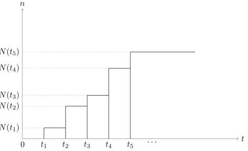
there are two types of counting processes with respect to the arrival rate. One with a constant increments or homogenousand one that experiences different arrival numbers, i.e. non-homogenous. Moreover, a counting process can be classified with respect to the time horizon domain. If the domain is discrete, we call the process discrete and countinuous, otherwise. Each discrete counting process can be divided into several subgroups, accord-ing to the distribution of the interarrival time, i.e. the distribution of the time between each pair of consecutive process values. From this perspective, a process can be clasified as periodic or aperiodic. The latter type is specialized even further following the specific distribution mass function. For instance, a Poisson counting process has an exponential interarrival distribution (see [49]).
n
t N(t1)
N(t2)
N(t3)
N(t4)
N(t5)
t1 t2 t3 t4 t5 . . .
0
Figure 2.1: Non-homogenous and periodic counting process.
The distribution of the number of arrivals at the system can be approximated by a counting process. Figure 2.1 depicts a general graph of a non-homogenous, periodic counting process. We used an instance of it to collect various statistics for the different time intervals (see Section 4.2.5). For each of them we studied the distributions of the order features (see Section 2.1) based on past data and then used the statistics to generate one hundred datasets of orders. Their goal is to simulate fleet activity and in this manner to allocate the vehicles in positions, which are better for handling the occurrence of possible unreserved demands.