UNIVERSIDADE DO ALGARVE
UNIVERSITY OF ALGARVE
FACULDADE DE CIÊNCIAS E TECNOLOGIA
FACULTY OF SCIENCES AND TECHNOLOGY
“Trophic Assessment in Chinese Coastal Systems”
MESTRADO EM GESTÃO DA ÁGUA E DA COSTA
(CURSO EUROPEU)
ERASMUS MUNDUS EUROPEAN JOINT MASTER
IN WATER AND COASTAL MANAGEMENT
Yongjin Xiao
NOME / NAME: Yongjin Xiao
DEPARTAMENTO / DEPARTMENT: Química, Bioquímica e Farmácia
ORIENTADOR / SUPERVISOR: Doutor João Gomes Ferreira, Professor Associado da Faculdade de Ciências e Tecnológica da Universidade Nova de Lisboa.
DATA / DATE: 16th February 2007
TÍTULO DA TESE / TITLE OF THESIS: Trophic Assessment in Chinese Coastal Systems
JURI Presidente:
Doutor Tomasz Boski, Professor Catedrático da Faculdade de Ciências do Mar e Ambiente da Universidade do Algarve;
Vogais:
Doutor José Pedro de Andrade e Silva Andrade, Professor Catedrático da da Faculdade de Ciências do Mar e Ambiente da Universidade do Algarve;
Doutor João Gomes Ferreira, Professor Associado da Faculdade de Ciências e Tecnológica da Universidade Nova de Lisboa;
Doutora Alice Newton, Professora Auxiliar da Faculdade de Ciências e Tecnologia da Universidade do Algarve.
ACKNOWLEDGEMENTS
First, I would like to sincerely acknowledge my supervisor, Professor João Gomes Ferreira, from whom I have received so much support and guidance throughout the project. I am grateful to Prof. Alice Newton, Erasmus Mundus programme and TAICHI project for supporting this work. Special thanks to Dr. Suzanne Bricker for her enthusiastic support, much good advice on methodological issues and reviewing this thesis. I would also like to express my appreciation to Prof. Mingyuan Zhu and Xuelei Zhang for their kind hosting and helpful discussion in Jiaozhou Bay, and João Pedro Nunes for his technological support in SWAT, GIS application and proof-reading this thesis. Finally, I owe a debt of gratitude to my family and my girlfriend who have never failed in encouraging me through the entire MSc. project.
RESUMO
Eutrofização costeira é definida como "o desenvolvimento de algas estimulado pelo o enriquecimento de nutrientes" em águas costeiras. Desde à duas décadas atrás, começou por ser uma das principais ameaças para as áreas costeiras Chinesas. A enorme quantidade de nutrientes a partir de actividades humanas tem modificado a qualidade natural da água dos estuários, baías e outras zonas costeiras. Como resultado, da sua elevada condição eutrofíca, os sistemas costeiros estão sujeitos a uma serie de impactos negativos com indesejáveis consequências, tais como, a mortalidade de peixes e a interdição da aquacultura de mariscos. Este assunto e de grande interesse na gestão costeira, existindo a necessidade de avaliar e identificar o nível eutrofíco em sistemas costeiros. Neste trabalho, os diferentes métodos de avaliação Chineses são discutidos e comparados com os do Ocidente, tais como, OSPAR, COMPP e ASSETS. ASSETS foi escolhido para dois estudos de (estuário de Changjiang e baía de Fiaozhou) devido à sua solida teoria e aplicações bem sucedidas. A metodologia é baseada no modelo pressão-estado-resposta e 3 índices: Influência humana, Condição Eutrófica, Tendências futuras. Os resultados obtidos para o estuário de Changjiang e a Baía de Fiaozhou, foram "Mau" e "Baixo" embora havia falta de dados, e são mais conclusivos que os resultados obtidos com métodos tradicionais. As comparações das fundamentações por trás das metodologias e dos resultados sugerem que o ASSETS poderá ser um método mais razoável e aplicável para avaliar os sistemas costeiros Chineses.
Palavra-chaves: Avaliação de Eutrofização; ASSETS; Estuário Changjiang; Baía Jiaozhou
ABSTRACT
Coastal eutrophication, mainly defined as ―the enrichment of nutrient stimulating algal growth‖ in coastal water, has started to be one of the main threats to the Chinese coastal areas since last two decades. The huge amount of nutrient loads from the human activities has modified the natural background of water quality in estuaries, bays and other coastal zones. As a result of elevated eutrophic status, coastal systems are subject to a series of negative and undesirable consequences, such as fish-kills and interdiction of shellfish aquaculture. While much attention is focused on managing this issue, there is a need to assess the eutrophic level in coastal systems and to identify the extent of danger. In this thesis, a variety of traditional Chinese assessment methods are discussed and compared with western ways, such as OSPAR COMPP and ASSETS. Afterwards, ASSETS was chosen to carry out two case studies (Changjiang Estuary and Jiaozhou Bay) due to its solid theory and successful applications. As a process-based method, it set up a pressure-state-response model based on three main indices, i.e., Overall Human Influence, Overall Eutrophic Condition and Future outlook. In spite of the lack of enough data, the results from applying ASSETS to Changjiang Estuary and Jiaozhou Bay are ―Bad‖ and ―Low‖ respectively, while the traditional methods only obtain more ambiguous results. The comparisons of the rationalities behind the methodologies and the results suggest that ASSETS could be a more reasonable and applicable method to assess Chinese coastal systems.
CONTENTS
Chapter 1. Introduction and objectives ··· 1
Chapter 2. Review of Chinese coastal systems ··· 7
Chapter 3. Review of eutrophication assessment methods ··· 16
3.1. Nutrient Index Method I ··· 17
3.2. Nutrient Index Method II ··· 17
3.3. Principal Component Analysis (PCA) ··· 18
3.4. Fuzzy Analysis ··· 20
3.4.1. Determination of membership function ··· 21
3.4.2. Determination of weights ··· 22
3.4.3. Fuzzy synthetic evaluation ··· 23
3.5. OSPAR COMPP ··· 24
3.5.1. Step One: Assessment parameters for classification ··· 26
3.5.2. Step Two: Integration of categorized assessment parameters for classification ··· 26
3.5.3. Step Three: Overall classification ··· 29
3.6. EPA NCR Water Quality Index ··· 29
3.6.1. Nutrients: nitrogen and phosphorus ··· 30
3.6.2. Chlorophyll a ···· 31
3.6.3. Water clarity ··· 32
3.6.4. Dissolved oxygen ··· 33
3.6.5. Calculating the water quality index ··· 34
3.7. ASSETS ··· 35
3.7.1. Data collection and synthesis ··· 36
3.7.2. State--Overall Eutrophic Condition (OEC) ··· 40
3.7.3. Pressure--Overall Human Influence (OHI) ··· 43
3.7.4. Response--Determination of Future Outlook (DFO) ··· 46
3.7.5. Synthesis--Overall grade ··· 47
Chapter 4. Case studies ··· 49
4.1. Changjiang Estuary ··· 55
4.1.1. Issues of concern: HABs and Hypoxia ··· 56
4.1.2. Homogeneous areas ··· 57
4.1.3. Data completeness and reliability ··· 58
4.1.4. Overall eutrophic Condition (OEC) ··· 58
4.1.5. Overall human influence (OHI) ··· 62
4.1.6. Future outlook ··· 74
4.1.7. Summary of the ASSETS indices ··· 75
4.2. Jiaozhou Bay ··· 77
4.2.1. Issues of concern ··· 78
4.2.2. Homogeneous areas ··· 79
4.2.3. Data completeness and reliability ··· 79
4.2.4. Overall eutrophic Condition (OEC) ··· 81
4.2.5. Overall human influence (OHI) ··· 86
4.2.6. Determination of Future Outlook (FO) ··· 91
4.2.7. Summary of the ASSETS indices ··· 92
4.3. Results ··· 94
4.3.1. Changjiang Estuary ··· 94
4.3.2. Jiaozhou Bay ··· 95
Chapter 5. Discussion of methodology ··· 49
5.1. Comparison among ―Phase I‖ and ―Phase II‖ methods ··· 49
5.2. Comparison among ―Phase II‖ methods ··· 50
Chapter 6. Conclusions ··· 97
Bibliography ··· 99
Chapter 1. Introduction and objectives
Eutrophication, considered as one of the major threats to the health of coastal systems for decades, has been redefined in a various ways. The word ―eutrophication‖ has its roots in two Greek words: ―eu‖ which means ―well‖ and ―trope‖ which means ―nourishment‖, while the modern use of the word eutrophication is related to inputs and effects of nutrients in aquatic systems (Andersen et al., 2006). The following paragraphs present some widely accepted definitions that are found in the literature. a. The definition adopted by U.K. Environment Agency is: ―the enrichment of
waters by inorganic plant nutrients which results in the stimulation of an array of symptomatic changes. These include the increased production of algae and/or other aquatic plants, affecting the quality of the water and disturbing the balance of organisms present within it. Such changes may be undesirable and interfere with water uses.‖ (U.K. Environment Agency, 1998)
b. The European Commission (EC) Urban Waste Water Treatment (UWWT) Directive defines eutrophication as ―the enrichment of water by nutrients, especially nitrogen and/or phosphorus, causing an accelerated growth of algal and higher form of plant life to produce an undesirable disturbance to the balance of organisms in the water and to the quality of water concerned‖ (91/271/EEC). c. According to US EPA, eutrophication is a ―condition in an aquatic ecosystem
where high nutrient concentrations stimulate blooms of algae (e.g., phytoplankton)‖ (http://www.epa.gov/maia/html/eutroph.html).
d. In the National Estuarine Eutrophication Assessment (NEEA) report conducted by NOAA, eutrophication refers to a process in which the addition of nutrients to water bodies stimulates algal growth (Bricker et al., 1999). And an updated definition from NEEA is a natural process by which productivity of a water body, as measured by organic matter, increases as a result of increasing nutrient inputs. These inputs are a result of a natural process but in recent decades they have been greatly supplemented by various human related activities (Bricker et al., 2004).
While eutrophication is getting more and more public and scientific attention all over the world, China is subject to a huge human-induced nutrient modification in coastal systems. One of the most significant changes is the increase of the nutrient inputs from land-source or human-related issues, resulting in the proliferation of phytoplanktonic biomass and algal blooms. Frequent occurrences of HABs (Fig. 1) and eutrophication have become serious issues in Chinese coastal systems (Harrison et al., 1990; Zhang et al., 1999; Huang et al., 2003). In 2003, the national sea waters witnessed altogether 119 cases of marine red tides, added up area bout 14.55 thousand square kilometers.
Fig.1. HAB incidents in coastal China from 1972 to 2004 (http://www.china-hab.cn).
Although it is argued that the main reason for this increased HAB incidents is the better national monitoring network, this record is also a clear indicator of more and more serious eutrophication in a national scale. As a result, nutrient enrichment may lead to negative and undesirable consequences, such as fish-kills, interdiction of shellfish aquaculture, loss or degradation of sea grass beds (Bricker et al., 2003). These effects strongly shape public concern and scientific research for better understanding of eutrophication (Cloern, 2001).
Even though there is no specific legislation designed to deal with eutrophication in China, the government has launched a series of laws and regulations to deal with the water-related problem. A list of the legislation related to water quality issues is summarized in Table 1.
Table 1 List of legislation related to water quality issues.
Title Objective Date
Regulations of the People’s Republic of China on the Prevention of Vessel-induced Sea
Pollution
To Protect marine environment 1983
The Water Pollution Control Act of People’s Republic of China
To control Inland water pollution 1984
Regulations of the People’s Republic of China on Control over Dumping of Wastes in the
Seawater
To regulate dumping of waste 1985
Regulations of the People’s Republic of China
on the Prevention of Pollution Damage to the Marine Environment by Land-sourced
Pollutants
To administrate land pollution sources
and to prevent pollution damage to the
marine environment by land-sourced
pollutants
1990
Regulation of the People’s Republic of China
on Controlling Marine Pollution by Inland Pollutants
To control marine pollution from inland
source
1990
Law of the People’s Republic of China on the Territorial Sea and the Contiguous Zone
To define and to protect territorial sea
and contiguous zone
1991
Decision of the State Council on several issues concerning environmental protection
To Strengthen the prevention and control
of water pollution in rivers and coastal
waters
Table 1 (continued)
Title Objective Date
Decision of the Standing Committee of the National People’s Congress on approval of the United Nations Convention on the Law of the
Sea
A full adoption of United Nations
Conventions on the Law of the Sea
(UNCLOS) treaty norms by China
1996
Law of People’s Republic of China on the Exclusive Economic Zone and Continental
Shelf
To define the Exclusive Economic Zone
and the continental shelf and to specify
the jurisdictional powers of China
1998
Seawater Quality Standard of the People’s Republic of China
To classify seawater quality into four
grades according to the standards set for
each grade
1998
Marine Environment Protection Act of People’s Republic of China
Marine environment protection 1999
Water Act of People’s Republic of China A general law for management,
utilization and protection of water
resources
2002
However, before the country sets political priorities for managing and mitigating nutrient enrichment, there is a need for China to make an assessment so as to determine the extent of the problem.
thesis is an attempt to go further in terms of understanding this issue. The main objectives in this thesis are:
To provide an overview of Chinese coasts regarding eutrophication conditions;
To review the eutrophication assessment methods and to compare them with methods used elsewhere;
To propose a rational and applicable method to better assess Chinese coastal systems;
To apply the method to two Chinese systems as a test of its wider applicability in China.
Chapter 2. Review of Chinese coastal systems
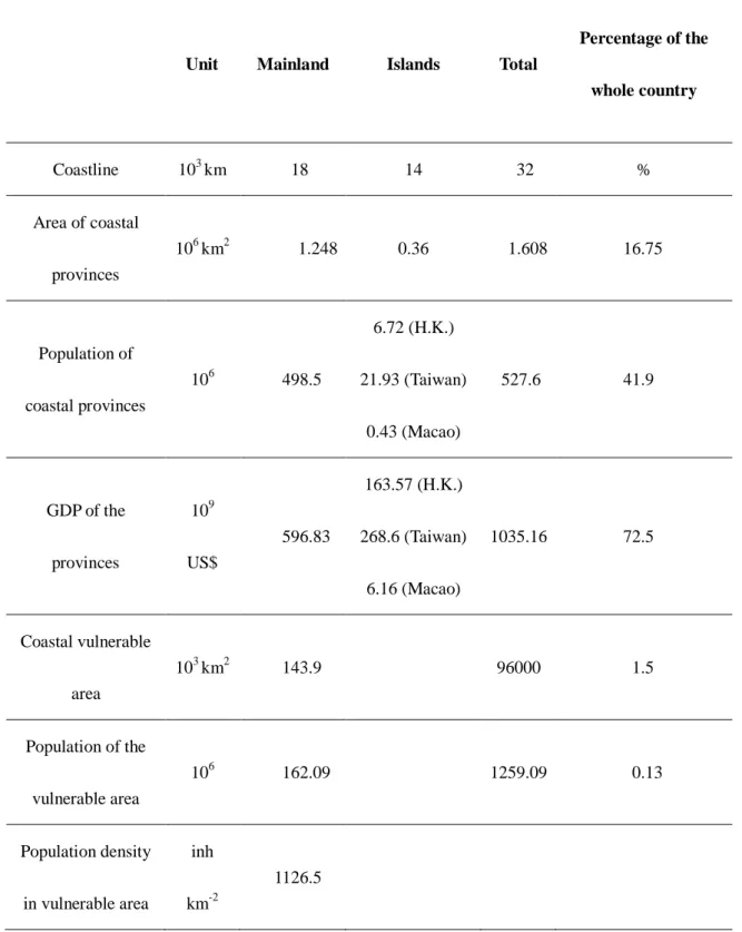
With an area of 2.85×10⁵ km2, roughly equivalent to the area of Portugal, Chinese coastal zones cover 23º of latitude (17ºN to 40ºN) and 16º of longitude (108ºE to 124.5ºE). Usually they are highly populated, economically developed, and thus the water bodies are often characterized by important anthropogenic nutrient loads (Table 2).
Out of various pressures to Chinese coastal systems, eutrophication is one of most negative factors influencing ecosystem health. The coastal areas of China that are a concern with harmful algal blooms are (from north to south) the Bohai Sea, the Yellow Sea, the East China Sea, and the South China Sea (Fig. 2). The first documented occurrence of a HAB was in the 1930s, and since then, reports of HABs appear to be increasing over time (Yan et al., 2003).
Table 2 Overview of Chinese coastal zone (adapted after Du et al., 1997; Li et al., 2000; P.R.C.
National Bureau of Statistics, 2000).
Unit Mainland Islands Total
Percentage of the whole country Coastline 103 km 18 14 32 % Area of coastal provinces 106 km2 1.248 0.36 1.608 16.75 Population of coastal provinces 106 498.5 6.72 (H.K.) 21.93 (Taiwan) 0.43 (Macao) 527.6 41.9 GDP of the provinces 109 US$ 596.83 163.57 (H.K.) 268.6 (Taiwan) 6.16 (Macao) 1035.16 72.5 Coastal vulnerable area 103 km2 143.9 96000 1.5 Population of the vulnerable area 106 162.09 1259.09 0.13 Population density in vulnerable area inh km-2 1126.5
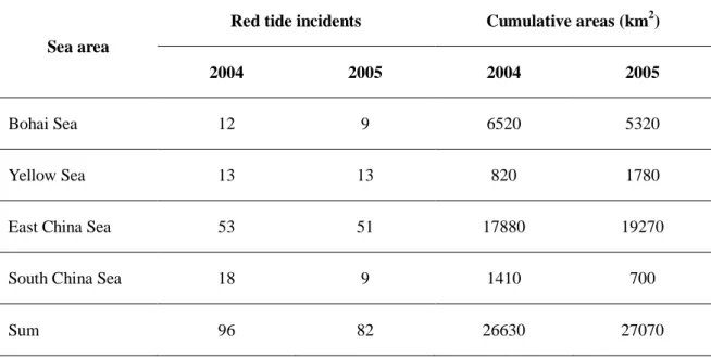
At a national scale, 82 red tides were reported in China during 2005 (Table 3) with a cumulative area of 27,070 km2 (State Oceanic Administration, 2006).
Table 3 Red tides reported in Chinese coasts during 2004 to 2005.
Sea area
Red tide incidents Cumulative areas (km2) 2004 2005 2004 2005
Bohai Sea 12 9 6520 5320
Yellow Sea 13 13 820 1780
East China Sea 53 51 17880 19270
South China Sea 18 9 1410 700
Sum 96 82 26630 27070
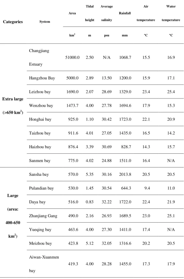
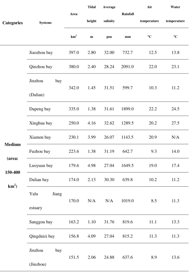
To understand the individual coastal systems in China, various data on Chinese bays and estuaries are listed as follows based on a series of Chinese documents called ―Bays in China‖. In this thesis, they are categorized into five groups in terms of areas (extra small, small, medium, large and extra large). Table 4 and 5 present the base data and synthesis data for major coastal systems collected from ―Bays in China‖ (for the smaller systems, see Annexes, Table 1).
Table 4 Background data for Chinese coastal systems. Categories System Area Tidal height Average salinity Rainfall Air temperature Water temperature km2 m psu mm ºC ºC Extra large (>650 km2) Changjiang Estuary 51000.0 2.50 N/A 1068.7 15.5 16.9 Hangzhou Bay 5000.0 2.89 13.50 1200.0 15.9 17.1 Leizhou bay 1690.0 2.07 28.69 1329.0 23.4 25.4 Wenzhou bay 1473.7 4.00 27.78 1694.6 17.9 15.3 Honghai bay 925.0 1.10 30.42 1723.0 22.1 20.9 Taizhou bay 911.6 4.01 27.05 1435.0 16.5 14.2 Haizhou bay 876.4 3.39 30.69 828.7 14.3 15.7
Sanmen bay 775.0 4.02 24.88 1511.0 16.4 N/A
Large (area: 400-650 km2) Sansha bay 570.0 5.35 30.16 2013.8 20.5 20.5 Pulandian bay 530.0 1.45 30.54 644.3 9.4 11.0 Daya bay 516.0 0.83 32.22 1722.0 22.4 21.9 Zhanjiang Gang 490.0 2.16 26.93 1689.5 23.0 25.1
Yueqing bay 463.6 4.00 27.30 1411.0 17.4 N/A
Meizhou bay 423.8 5.12 32.05 1316.6 20.2 20.5
Aiwan-Xuanmen
bay
Table 4 (continued) Categories Systems Area Tidal height Average salinity Rainfall Air temperature Water temperature km2 m psu mm ºC ºC Medium (area: 150-400 km2) Jiaozhou bay 397.0 2.80 32.00 732.7 12.5 13.8 Qinzhou bay 380.0 2.40 28.24 2091.0 22.0 23.1 Jinzhou bay (Dalian) 342.0 1.45 31.51 599.7 10.3 11.2 Dapeng bay 335.0 1.38 31.61 1899.0 22.2 24.5 Xinghua bay 250.0 4.16 32.62 1289.5 20.2 27.5
Xiamen bay 230.1 3.99 26.07 1143.5 20.9 N/A
Fuzhou bay 223.6 1.38 31.19 642.7 9.3 14.0 Luoyuan bay 179.6 4.98 27.04 1649.5 19.0 17.4 Dalian bay 174.0 2.13 30.30 639.8 10.2 11.2 Yalu Jiang estuary 170.0 N/A N/A 1019.0 8.5 11.3 Sanggou bay 163.2 1.10 31.76 819.6 11.1 13.3 Qingduizi bay 156.8 4.09 27.04 815.2 11.3 11.3 Jinzhou bay (Jinzhou) 151.5 2.06 24.88 637.6 8.9 13.6
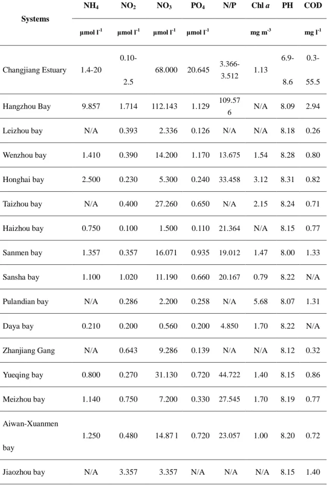
Table 5 Synthesis data for Chinese coastal systems.
Systems
NH4 NO2 NO3 PO4 N/P Chl a PH COD
μmol l-1 μmol l-1 μmol l-1 μmol l-1
mg m-3 mg l-1 Changjiang Estuary 1.4-20 0.10- 2.5 68.000 20.645 3.366- 3.512 1.13 6.9- 8.6 0.3- 55.5 Hangzhou Bay 9.857 1.714 112.143 1.129 109.57 6 N/A 8.09 2.94 Leizhou bay N/A 0.393 2.336 0.126 N/A N/A 8.18 0.26
Wenzhou bay 1.410 0.390 14.200 1.170 13.675 1.54 8.28 0.80
Honghai bay 2.500 0.230 5.300 0.240 33.458 3.12 8.31 0.82
Taizhou bay N/A 0.400 27.260 0.650 N/A 2.15 8.24 0.71
Haizhou bay 0.750 0.100 1.500 0.110 21.364 N/A 8.15 0.77
Sanmen bay 1.357 0.357 16.071 0.935 19.012 1.47 8.00 1.33
Sansha bay 1.100 1.020 11.190 0.660 20.167 0.79 8.22 N/A
Pulandian bay N/A 0.286 2.200 0.258 N/A 5.68 8.07 1.31
Daya bay 0.210 0.200 0.560 0.200 4.850 1.70 8.22 N/A
Zhanjiang Gang N/A 0.643 9.286 0.139 N/A N/A 8.12 0.32
Yueqing bay 0.800 0.270 31.130 0.720 44.722 1.40 8.15 0.86
Meizhou bay 1.140 0.750 7.200 0.330 27.545 1.70 8.19 0.77
Aiwan-Xuanmen
bay
1.250 0.480 14.87 l 0.720 23.057 1.00 8.20 0.72
Table 5 (continued)
Systems
NH4 NO2 NO3 PO4 N/P Chl a PH COD
μmol l-1 μmol l-1 μmol l-1 μmol l-1
mg m-3 mg l-1
Qinzhou bay N/A 0.071 2.786 0.645 N/A N/A 7.77 0.78
Jinzhou bay
(Dalian)
N/A 0.003 0.003 0.548 N/A 3.17 8.19 0.65
Dapeng bay 2.530 0.140 4.570 0.090 80.444 2.25 8.20 0.92
Xinghua bay 0.400 0.220 1.020 0.100 16.400 2.34 8.22 N/A
Xiamen bay 3.860 1.430 8.940 0.480 29.646 4.55 8.22 1.23
Fuzhou bay N/A 0.107 0.107 0.419 N/A 2.28 8.00 1.15
Luoyuan bay 1.480 0.970 8.680 0.290 38.379 2.01 8.23 N/A
Dalian bay N/A 3.386 7.786 1.000 N/A N/A 8.16 1.27
Yalu Jiang estuary N/A N/A N/A 0.460 N/A N/A 8.02 2.34
Sanggou bay N/A 92.857 457.143 403.226 N/A N/A 8.20 1.20
Qingduizi bay N/A 0.386 2.093 0.516 N/A N/A 8.11 1.41
Jinzhou bay
(Jinzhou)
N/A N/A N/A N/A N/A 3.10 8.00 1.30
Quanzhou bay 5.700 1.020 29.300 0.300 120.067 1.43 7.94 1.08
Tong-an bay 4.150 0.720 14.200 0.200 95.350 2.00 8.25 1.02
Shidao bay 0.571 0.500 3.643 0.032 146.143 N/A 8.08 1.32
Table 5 (continued)
Systems
NH4 NO2 NO3 PO4 N/P Chl a PH COD
μmol l-1 μmol l-1 μmol l-1 μmol l-1
mg m-3 mg l-1
Shantou Gang 6.800 4.200 38.000 0.490 100.000 4.50 7.84 2.02
Rongcheng bay N/A 1.143 0.043 0.452 N/A N/A 8.13 0.80
Xiaoyao bay N/A 0.236 1.193 0.355 N/A N/A 8.19 0.81
Anpu Gang N/A 0.279 0.214 0.084 N/A N/A 8.85 0.63
Dongshan bay 0.870 0.420 6.070 0.380 19.368 3.22 8.24 1.07
Guanhe mouth N/A N/A 0.910 1.300 N/A N/A 8.20 N/A
Hai He estuary N/A N/A N/A N/A N/A N/A 8.00 N/A
Huang He estuary 0.927 0.429 5.556 0.197 35.086 N/A 8.25 1.62
Laoshan bay N/A N/A N/A N/A N/A N/A N/A N/A
Liao He estuary 0.001 0.006 0.086 0.790 0.118 N/A 7.91 3.06
Lingshan bay N/A N/A N/A N/A N/A N/A N/A N/A
Luan He estuary 0.570 0.230 1.270 0.510 4.059 N/A 8.20 N/A
Majia He estuary N/A N/A N/A N/A N/A N/A N/A N/A
Minjiang estuary 6.400 1.310 44.200 1.500 34.607 2.40 7.60 2.53
Pearl River estuary N/A N/A N/A 0.980 N/A N/A 8.15 N/A
Tuhai He estuary N/A N/A N/A N/A N/A N/A N/A N/A
Wuleidao bay N/A N/A N/A N/A N/A N/A N/A N/A
Although a national trophic assessment of Chinese coastal systems has not conducted yet, it is highly suspected that most of coastal areas and estuaries are suffering from overloaded nutrients. The available literature suggests that those undergoing most severe eutrophication include Bohai Bay, Changjiang Estuary, Hangzhou Bay and Pearl River Estuary (Zou et al., 1985; Peng & Wang, 1991; Pei & Ma, 2002; Chai et al., 2006).
Chapter 3. Review of eutrophication assessment methods
Eutrophication assessment, began with classical freshwater approach (Carlson, 1977; Morihiro et al., 1981), has developed through two ―phases‖ (Cloern, 2001). These nutrient-based classification systems are termed as a ―Phase I‖ approach due to developing through the measurement of variables such as transparency, nutrients and chlorophyll a. Over the last few decades, the increase in research effort and discussion on coastal eutrophication processes has advanced our understanding of the problems, and increasingly effective ―Phase II‖ methods have been developed to explore cause/effect relationships, such as the Oslo-Paris (OSPAR) Convention for the Protection of the North Sea Comprehensive Procedure (OSPAR COMM), US EPA’s National Coastal Assessment (NCA) water index method and Assessment of Estuarine Trophic Status (ASSETS) method (Weisberg et al., 1993; Lowery, 1996; Madden and Kemp, 1996; Bricker et al., 1999; Dettmann, 2001; EPA, 2005).
In the Chinese history of eutrophication assessment, there are a number of eutrophication assessment methods proposed in China, such as the nutrient index and fuzzy analysis. As they mainly focus on the pressures to the systems by chemical tools, these methods are usually cited as ―Phase I‖ approaches (Wang, 2005; Yao, 2005). A subset of these methods which are commonly used is reviewed in this chapter, such as Nutrient Index Method, Primary Component Analysis and Fuzzy Analysis.
In addition, three other methods, the OSPAR-COMPP (developed by the OSPAR signatories), NCR Water Quality Index (US EPA National Coastal Report) and ASSETS (US NOAA) are outlined as well. Even though they have only incompletely
been applied to Chinese systems, these approaches might be helpful to present a different way to look at Chinese eutrophication issues.
3.1. Nutrient Index Method I
The method suggested by Chinese National Environmental Monitoring Center is based on nutrient index.
Nutrient Index (NI) in seawater (Lin, 1996) is calculated by Eq.1:
NI=CCOD/SCOD + CTN/STN + CTP/STP + CChla/SChla (Eq. 1)
where: CCOD, CTN, CTP and CChla are measured concentrations of COD, total
nitrogen, total phosphorus (in mg l-1) and chlorophyll a (in μg l-1) in sea water, respectively. SCOD, STN, STP and SChla are standard concentrations of COD, total
nitrogen, total phosphorus and chlorophyll a in sea water, respectively (Table 6).
NI, if larger than 4, indicates the sea water is eutrophic.
Table 6 Seawater eutrophication assessment standards (Lin, 1996).
SCOD STN STP SChla
3.0 mg l-1 0.6 mg l-1 0.03 mg l-1 10 μg l-1
3.2. Nutrient Index Method II
Adapted from Japanese assessment methods (Okaichi, 2004), Zou and his colleagues proposed one other nutrient index method (Zou et al., 1985).
Nutrient Index (NI) in seawater:
where CCOD, CDIN, CDIP are measured concentrations of COD (in mg l-1), dissolved
inorganic nitrogen and phosphorus in seawater, respectively.
4500/106 in Eq. 2 is mean product of standard concentrations of COD, DIN and DIP, as it is believed that the critical value for COD is 1-3 mg l-1, DIN 0.2-0.3 mg l-1 and DIP 0.01-0.02 mg l-1 (Chen et al., 2002).
NI, if larger than 1, indicates the sea water is eutrophic.
These two limnology-originated methods mentioned above are simple to carry out, with parameters easy to sample. While they are widely used in Chinese coastal systems, research in the past decades has identified key differences in the responses of lakes and coastal-estuarine ecosystems to nutrient enrichment (Cloern, 2001). In addition, it is widely accepted nowadays that nitrogen and phosphorus concentration are not necessarily indicative of coastal eutrophication.
3.3. Principal Component Analysis (PCA)
The basic philosophy underlying this method is that traditionally sampled eutrophic parameters are correlated to each other, and there is a need to find out the principal components out of various variables. Two main types of trophic indicators have been and are still being used in eutrophication assessment, i.e., biological factors and physico-chemical factors (Parinet el al., 2004). Even though the specific cause and effect relation between these factors are not clear yet, it’s obvious that they are connected to each other (Strain & Yeats, 1999). Given the complexity of the system, the aim of this method is to apply linear regression to make up a set of information
that could provide a more reliable way to characterize the state of the aquatic system than variables themselves.
Here are two examples of principal components selected through PCA method from the literature:
a. Lin and her colleagues analyzed data from Zhelin Bay (Guangdong Province, China) and selected four parameters, i.e., water temperature, salinity, concentration of PO4 and SiO3, which represent up to 91.46% of the total variance
of the observance (Lin et al., 2004).
b. In Parinet’s work done in 2004, the data base for 18 eutrophic variables from ten lakes in Ivory Coast were interpreted and it was suggested that four parameters, conductivity, pH, permanganate index and UV absorbance, were possible to make a precise description without impairing its quality (Parinet et al., 2004).
The conduction of PCA obtains a few variables with which the system is able to be simplified to assess with not missing main information. After being calibrated, the selection of principal parameters could be extended to a larger area of water systems.
The advantage of this method is obvious, that is, it needs fewer parameters to be sampled after making principal components analysis. While it’s common that most of coastal systems face data gaps, it allows scientists or managers to better make use of data available. Combined with Nutrient Index Methods, PCA is able to find out the most important parameters related to the eutrophic conditions, which provides a more flexible way than using the parameters from Nutrient Index methods themselves. However, since it is based on statistic calculation, PCA does not have solid scientific
basis in coastal science, but only empirical statistical rationality. This is probably the main reason that it has not been commonly applied to Chinese system.
3.4. Fuzzy Analysis
The main advantage that fuzzy theory has is its ability to deal with imprecise, uncertain or ambiguous data or relationship, which is clearly fit to the study of ecological and environmental issues (Metternicht, 2001).
In most conventional methods, a variety of threshold values are used to give a classification for parameters when evaluating the system status. However, a discrepancy frequently arises from the lack of a clear distinction between the uncertainty in the quality criteria employed and the vagueness or fuzziness embedded in the decision-making output values (Chang et al., 2001). Owing to inherent imprecision, difficulties always exist in describing eutrophic conditions through distinct numbers used as thresholds for various variables.
In early developed eutrophication index methods, such as Calson’s index, tended to divide eutrophication level by discrete numbers (Calson, 1977). For example, Trophic State Index values of 49 and 50 are in different classes while 41 falls into the same category with 49, even though it sounds much more reasonable to put 49 and 50 together. In this case, Fuzzy theory seems to be a possible solution to deal with the ambiguity within eutrophication assessment. Although the theory had existed for decades, to apply fuzzy theory to assess water quality began in the 1990s (Peng et al., 1991; Kung et al., 1992; Salski, 1992; Lu & Lo, 2002; Marchini & Marchini, 2006).
3.4.1. Determination of membership function
Suppose there are n sampling sites, which collected m parameters, such as dissolved inorganic nitrogen, chlorophyll a and dissolved oxygen. Then the dataset could be written down as the following matrix:
Multivariable data: ) ( ... .. ... ... ... ... ... 2 1 2 22 21 1 12 11 ij mn m m n n x x x x x x x x x x X (Eq. 3) where i = 1, 2, …, m; j = 1, 2, …, n.
Assume that water quality standards are divided into c categories, for example, trophic levels like low, medium and high. Then the multivariable index can be written as the following matrix.
Multivariable index: ) ( ... .. ... ... ... ... ... 2 1 2 22 21 1 12 11 ih mc m m c c y y y y y y y y y y Y (Eq. 4) where i = 1, 2, …, m; j = 1, 2, …, n; h = 1, 2, …, c.
To define the membership of multivariable index as following, respectively, increasing (yi1 < yic) and decreasing (yi1 > yic):
c h c h h y y y yih i ic i ih 1 1 , 1 ), /( ) ( , 0 1 1 (Eq. 5) and
c h c h h y y y yih ic i ic ih 1 1 , 1 ), /( ) ( , 0 1 (Eq. 6)
Named θij the general membership function for xij, it can be obtained as the
following analytical expressions, respectively, increasing (yi1 < yic) and decreasing
(yi1 > yic): ic ij ic ij i i ij i ic i ij ij y x y x y y x y y y x 1 1 1 1 , 1 ), /( ) ( , 0 (Eq. 7) and 1 1 1 , 1 ), /( ) ( , 0 i ij i ij ic ic ij ic i ic ij ij y x y x y y x y y y x (Eq. 8) 3.4.2. Determination of weights
The over standard weight of xij (oij) is calculated by the following formula:
) 1 /( / 1
c h ih ij i ij ij y c x y x o (Eq. 9)On the other hand, different variables are of various importance to water quality. For example, nitrogen concentration and phosphorus concentration might be more clear indicators than the water clarity for some aquatic systems in terms of eutrophication. Named vi the weight of parameters i, the synthesis weight set derives
from the product of oij and vi.
mn m m n n m o o o o o o o o o v v v W ... ... ... ... ... ... ... ... 2 1 2 22 21 1 12 11 2 1 (Eq. 10)
A normalized matrix is determined by normalizing the initial matrix W column by column. ) ( ... ... ... ... ... ... ... 2 1 2 22 21 1 12 11 ij mn m m n n w w w w w w w w w w W (Eq. 11)
where wij is the normalized synthesis weight for xij.
3.4.3. Fuzzy synthetic evaluation
When membership function and weight are given, fuzzy synthetic evaluation for site j to Level h can be performed as follows:
c k p m i p ik ij ij m i p ih ij ij jh w w e 1 / 2 1 1 ) ( ) ( 1 (Eq. 12)Then the overall trophic level can be presented by a matrix:
nc n n c c jh e e e e e e e e e e E ... .. ... ... ... ... ... ) ( 2 1 2 22 21 1 12 11 (Eq. 13)
where P is the fuzzy distance constant, equal to 1 (Hamming distance) or 2 (Euclidean distance) (Xiong & Chen, 1993).
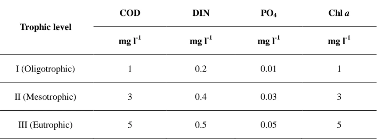
For example, Lin and his colleagues’ work applied the fuzzy analysis in Fujian sea area, China (Lin et al., 2002). In Xunjiang River, surface water samples were taken from five sampling sites, with four parameter studied, i.e., concentrations of PO4, DIN,
chlorophyll a and COD. The water quality standards used in this study were adopted from Chinese national seawater standards (Table 7).
Table 7 Assessment standard values. Trophic level COD DIN PO4 Chl a mg l-1 mg l-1 mg l-1 mg l-1 I (Oligotrophic) 1 0.2 0.01 1 II (Mesotrophic) 3 0.4 0.03 3 III (Eutrophic) 5 0.5 0.05 5
Setting P=1, the result of eutrophic level membership of surface water at Xunjiang River is shown as following matrix:
070 . 0 042 . 0 077 . 0 040 . 0 229 . 0 644 . 0 903 . 0 867 . 0 891 . 0 0699 . 0 286 . 0 055 . 0 056 . 0 069 . 0 072 . 0 5 4 3 2 1 III II I Site Site Site Site Site el TrophicLev E
The probabilities for these five sampling sites ranged from 64.4% to 90.3%, which suggested that studying area fell into the category of Level II.
Despite the great efforts in developing the application of fuzzy theory based on ecological models, the progress is still frustrating for mainly two reasons (Kompare et al., 1994; Chen & Mynett, 2003). The first one is large and redundant ruleset in high dimensional systems, the size of which grows exponentially with the number of variables. The other one is difficulties in defining membership functions and inference rules.
3.5. OSPAR COMPP
eutrophication status of the OSPAR Maritime Area (OSPAR, 2003). As a stepwise method, the OSPAR COMPP comprises two main procedures: the Screening Procedure and the Comprehensive Procedure. The Screening Procedure, as a ―broad-brush‖ approach, is designed to identify obvious non-problem areas with regard to eutrophication. Areas that are not identified as obvious non-problem areas in the first procedure are to be subjected to the Comprehensive Procedure to be classified into problem areas, potential problem areas or non-problem areas. These three types of areas with regard to eutrophication are defined as following:
a. ―Problem areas with regard to eutrophication‖ are those areas for which there is evidence of an undesirable disturbance to the marine ecosystem due to anthropogenic enrichment by nutrients;
b. ―Potential problem areas with regard to eutrophication‖ are those areas for which there are reasonable grounds for concern that the anthropogenic contribution of nutrients may be causing or may lead in time to an undesirable disturbance to the marine ecosystem due to elevated levels, trends and/or fluxes in such nutrients; c. ―Non-problem areas with regard to eutrophication‖ are those areas for which there
are no grounds for concern that anthropogenic enrichment by nutrients has disturbed or may in the future disturb the marine ecosystem.
In OSPAR COMPP system e.g. the frequency and spatial coverage of all parameters depend on the classification of the areas (problem area, potential problem area, non-problem area).
of steps should be undertaken which are described in the next section.
3.5.1. Step One: Assessment parameters for classification
In 2001 OSPAR adopted common harmonized assessment criteria and their respective (region-specific) assessment levels, which are presented in Table 8 (OSPAR, 2003).
The first step is to provide a score (+) for each of the harmonized assessment criteria being applied according to the commission-agreed guidance. For example, Category I is scored ―+‖ in cases where one or more of its respective assessment parameters is showing an increased trend or elevated change.
3.5.2. Step Two: Integration of categorized assessment parameters for classification
The second step is to integrate those scores obtained from the first step together to provide a coherent classification of the area (Table 9). For each assessment parameter from four categories, it can be indicated whether its measured concentration relates to a problem area, a potential problem area or a non-problem area as defined.
Table 8 The agreed harmonized assessment parameters of the Comprehensive Procedure (adapted
after OSPAR, 2003).
Categories Parameters
Criteria thresholds for elevated eutrophic status Category I Degree of nutrient enrichment Riverine TN and TP; direct discharge
Elevated inputs and/or increased
trends
Winter DIN and DIP
concentrations
Conc.>50% above background
conc. Winter N/P ratio >25 Category II Direct effect of nutrient enrichment
Maximum and mean Chl.
a concentration
Conc. >50% above background
conc.
Region specific
phytoplankton indicator
species
Elevated levels and increased
duration
Macrophytes
Shift from long-lived to
short-lived nuisance species
Category III Indirect effect of nutrient enrichment Degree of oxygen deficiency <2 mg l-1: acute toxicity; 2-6 mg l-1: deficiency Changes/kills in
zoobenthos and fish kills
Kills; long term changes in
zoobenthos biomass and species
composition
Table 8 (continued)
Categories Parameters
Criteria thresholds for elevated eutrophic status
Category
IV
Other possible effect of
nutrient enrichment
Algal toxins Incidence
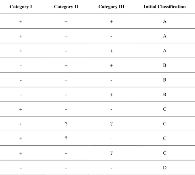
Table 9 Integration of categorized assessment parameter criteria.
Category I Category II Category III Initial Classification
+ + + A + + - A + - + A - + + B - + - B - - + B + - - C + ? ? C + ? - C + - ? C - - - D
(+) = Increased trends, elevated levels, shifts or changes in the respective assessment parameters in Table 9.
respective assessment parameters in Table 9.
(?) = Not enough data to perform an assessment or the data available is not fit for the purpose.
A=Problem area; B=Problem area or caused by transport from other parts of the maritime area; C=Potential problem area; D=Non-problem area.
3.5.3. Step Three: Overall classification
The third step is to make an appraisal of all relevant information (concerning the harmonized assessment criteria their respective assessment levels and the supporting environmental factors), to provide a transparent and sound account of the reasons for establishing a particular status for the area.
Supporting environmental factors and region specific characteristics should be taken into account, such as physical and hydrodynamic aspects, and weather/climate conditions. These region specific characteristics play a role in explaining the results of the area classification, and also, they are vital to identify a ―final classification‖.
3.6. EPA NCR Water Quality Index
To summarize the condition of ecological resources in the coastal waters of the United States, US Environmental Protection Agency (EPA) developed a Water Quality Index in National Coastal Condition Report II (NCCR II).
The water quality index is made up of five indicators: nitrogen, phosphorus, chlorophyll a, water clarity and dissolved oxygen.
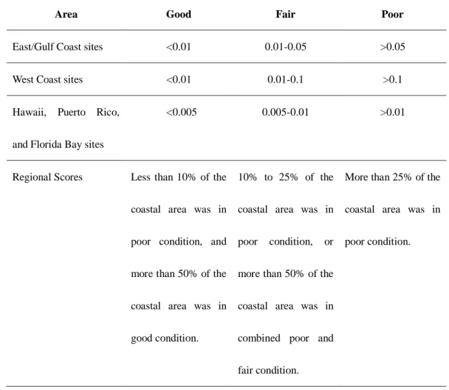
3.6.1. Nutrients: nitrogen and phosphorus
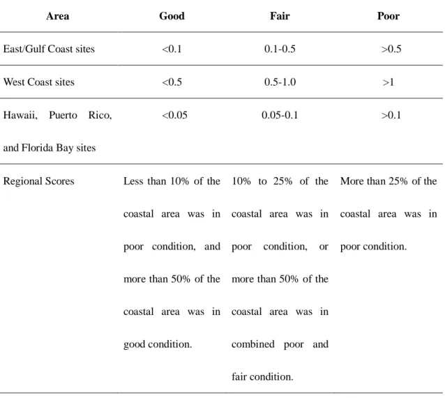
Coastal monitoring sites were rated good, fair, or poor for DIN and DIP, using the criteria shown in Table 10 and table 11. These rating were then used to calculate an overall rating for each region.
Table 10 Criteria for assessing dissolved inorganic nitrogen (all values in mg l-1).
Area Good Fair Poor
East/Gulf Coast sites <0.1 0.1-0.5 >0.5
West Coast sites <0.5 0.5-1.0 >1
Hawaii, Puerto Rico,
and Florida Bay sites
<0.05 0.05-0.1 >0.1
Regional Scores Less than 10% of the
coastal area was in
poor condition, and
more than 50% of the
coastal area was in
good condition.
10% to 25% of the
coastal area was in
poor condition, or
more than 50% of the
coastal area was in
combined poor and
fair condition.
More than 25% of the
coastal area was in
Table 11 Criteria for assessing dissolved inorganic phosphorus (all values in mg l-1).
Area Good Fair Poor
East/Gulf Coast sites <0.01 0.01-0.05 >0.05
West Coast sites <0.01 0.01-0.1 >0.1
Hawaii, Puerto Rico,
and Florida Bay sites
<0.005 0.005-0.01 >0.01
Regional Scores Less than 10% of the
coastal area was in
poor condition, and
more than 50% of the
coastal area was in
good condition.
10% to 25% of the
coastal area was in
poor condition, or
more than 50% of the
coastal area was in
combined poor and
fair condition.
More than 25% of the
coastal area was in
poor condition.
3.6.2. Chlorophyll a
In NCCR II, surface concentrations of chlorophyll a were determined from a filtered portion of water collected at each site and were rated good, fair, or poor using the criteria shown in Table 12.
Table 12 Criteria for assessing chlorophyll a (all values in μg l-1).
Area Good Fair Poor
East/Gulf Coast sites <5 5-20 >20
West Coast sites <0.5 0.5-1.0 >1
Hawaii, Puerto Rico,
and Florida Bay sites
<1 1-5 >5
Regional Scores Less than 10% of the
coastal area was in
poor condition, and
more than 50% of the
coastal area was in
good condition.
10% to 20% of the
coastal area was in
poor condition, or more
than 50% of the coastal
area was in combined
poor and fair condition.
More than 20% of
the coastal area was
in poor condition.
3.6.3. Water clarity
Water clarity was estimated by using specialized equipment that compares the amount and type of light reaching the water surface to the light at a depth of 1 meter, as well as by using a Secchi disk. Water clarity varies naturally among the various parts of American land; therefore, the water clarity indicator (WCI) is based on a ratio of observed clarity to regional reference conditions:
WCI = (observed clarity at 1 meter) / (regional reference clarity at 1 meter) Table 13 summarizes the rating criteria for water clarity for the regions.
Table 13 Criteria for assessing water clarity.
Area Good Fair Poor
Individual sampling sites WCI >2 WCI=1-2 WCI<1
Regional Scores Less than 10% of the
coastal area was in
poor condition, and
more than 50% of the
coastal area was in
good condition.
10% to 25% of the
coastal area was in poor
condition, or more than
50% of the coastal area
was in combined poor
and fair condition.
More than 25%
of the coastal
area was in poor
condition.
3.6.4. Dissolved oxygen
Dissolved oxygen was rated good, fair, or poor using the criteria shown in Table 14.
Table 14 Criteria for assessing dissolved oxygen.
Area Good Fair Poor
Individual sampling sites >5 mg l-1 2-5 mg l-1 <2 mg l-1
Regional Scores Less than 10% of the
coastal area was in
poor condition, and
more than 50% of the
coastal area was in
good condition.
10% to 25% of the coastal
area was in poor
condition, or more than
50% of the coastal area
was in combined poor and
fair condition.
More than 25%
of the coastal
area was in poor
3.6.5. Calculating the water quality index
With the data on DIN, DIP, chlorophyll a, water clarity, and dissolved oxygen, the water quality index rating is able to be calculated using the criteria shown in Table 15.
Table 15 Criteria for determining the water quality.
Rating Criteria
Good A maximum of one indicator is fair, and no indicators are poor.
Fair One of the indicators is rated poor, or two or more indicators are rated fair.
Poor Two or more of the five indicators are rated poor.
Missing Two components of the indicators are missing, and the available indicators do not
suggest a fair or poor rating.
The water quality index was then calculated for each region using the criteria in Table 16.
Table 16 Criteria for determining the water quality index rating by region.
Rating Criteria
Good Less than 10% of the coastal area was in poor condition, and more than 50% of the
coastal area was in good condition.
Fair 10% to 20% of the coastal area was in poor condition, or more than 50% of the coastal
area was in combined poor and fair condition.
3.7. ASSETS
ASSETS (the Assessment of Estuarine Trophic Status) is developed by the United States National Estuarine Eutrophication Assessment (NEEA), which was applied to 138 estuaries in the US. ASSETS is a more sophisticated and integrated methodology for eutrophication assessment in coastal zones, which may be applied comparatively to rank the eutrophication status of estuaries and coastal areas.
The concepts underlying ASSETS approach includes quantitative and semi-quantitative components, and uses field data, models and expert knowledge to evaluate Pressure-State-Response (PSR) indicators (Fig. 3). The core methodology relies on three diagnostic tools: a heuristic index of pressure (Overall Human Influence), a symptoms-based evaluation of state (Overall Eutrophic Conditions) and an indicator of management response (Definition of Future Outlook). It combines primary and secondary symptoms to derive an OEC index, which is then associated with a measure of OHI and the DFO.
Fig.3. Flow chart of ASSETS methodology (adapted from Bricker, 2003).
ASSETS may be divided into two parts: data collection and compilation, and application of indices. The step-by-step methodology is briefly reviewed in the following sections.
3.7.1. Data collection and synthesis
The data collection framework could be divided into three parts: division of estuaries into homogeneous areas, data collection, and evaluation of data completeness and reliability.
3.7.1.1. Physical division
The first step in applying the methodology is a physical classification of an estuarine system in terms of salinity. Each parameter was characterized for three salinity zones as defined in the NOAA’s National Estuarine Inventory (NEI): tidal fresh (0-0.5 psu), mixing (0.5-25 psu), and seawater (> 25 psu).
3.7.1.2. Data collection
Five variables from an original list of sixteen nutrient related water quality parameters are used for the assessment (Table 17; for a full description, see Bricker et al., 1999). According to Bricker et al. (2003), these eutrophication indicators were selected in order to:
a. be able to accurately characterize eutrophic conditions among highly varied systems; and to
Table 17 List of parameters considered in ASSETS.
Parameters Existing conditions
Chlorophyll a
a. Surface concentrations:
b. Limiting factors to algal biomass (N, P, Si, light, other)
c. Spatial coverage1; month of occurrence; frequency of occurrence2
Nuisance algae/toxic
algae
a. Occurrence: problem (significant impact upon biological
resources); no problem (no significant impact)
b. Dominant species
c. Event duration (hours, days, weeks, seasonal, other)
d. Months of occurrence; frequency of occurrence2
Macroalgae
a. Abundance: problem (significant impact upon biological
resources); no problem (no significant impact)
b. Months of occurrence; frequency of occurrence2
a. Anoxia (0 mg l-1)
b. Hypoxia (0-2 mg l-1)
c. Biological stress
(2-5 mg l-1)
a. Dissolved oxygen condition: observed; no occurrence
b. Stratification (degree of influence): high; medium; low; not a
factor
c. Water column depth: surface, bottom, throughout water column
d. Spatial coverage1; month of occurrence; frequency of occurrence2
Submerged aquatic
vegetation/
intertidal wetlands
Notes:
1) Spatial coverage (% of salinity zone): high (50-100%); medium (25-50%); low (10-25%); no
SAV/wetland in system
2) Frequency of occurrence: episodic (conditions occur randomly); periodic (conditions occur
annually or predictably); persistent (conditions occur continually throughout the year)
3.7.1.3. Analysis of data completeness and reliability
For each of these parameters, information on characteristics of timing, duration, spatial coverage, and frequency of occurrence are also collected as appropriate. Before compiling information for these parameters, there is a need to examine data gaps or speculative inferences. An analysis of data completeness and reliability (DCR) is carried out to inter-calibrate the spatial and temporal quality of the datasets and the confidence in the results. DCR is calculated by using the following combinations of parameter characteristics:
1) DCR (Chlorophyll a) = Concentration×Spatial Coverage×Frequency×Reliability; DCR (Macroalgae) = Concentration×Frequency×Reliability
DCR (Diss. oxygen) = Concentration×Spatial Coverage×Frequency×Reliability DCR (SAV) =Direction of change×Magnitude×Reliability
DCR (Nuisance algae) = Concentration×Frequency×Duration×Reliability DCR (Toxic algae) = Concentration×Frequency×Duration×Reliability
2) A rating based on the DCR score is assigned to each parameter and to the entire system as: high (75-100%); medium (50-74); low (0-49).
3) The entire system DCR value is then computed as the mean of the parameter DCRs.
3.7.2. State--Overall Eutrophic Condition (OEC)
The OEC index has a sequential approach based on two groups of symptoms, which bring together a subset of five parameters (Fig. 4).
The primary symptoms
correspond to the early stage of water quality degradation, which are examined through the analysis of chlorophyll a concentrations and macroalgal blooms.
Fig.4. Conceptual model of OEC (adapted after
Bricker et al., 2003).
In some systems, the primary symptoms lead to well developed eutrophic conditions, i.e., secondary (advanced) symptoms, such as submerged aquatic vegetation (SAV) loss, nuisance and toxic algal blooms and low dissolved oxygen (anoxia or hypoxia).
In the previous application of ASSETS, the epiphyte abundance was considered as one of the primary symptom. However, it would not be taken into account because of the lack of standard measure and conceptual overlapping with the SAV indicator,
which reflects the level of epiphyte colonization in a large part.
To combine results for this subset of symptoms into an indicator of OEC, concentration, spatial coverage, frequency of occurrence of extreme or problem occurrences are considered for a logic stepwise decision method.
3.7.2.1. Primary symptoms method (PSM)
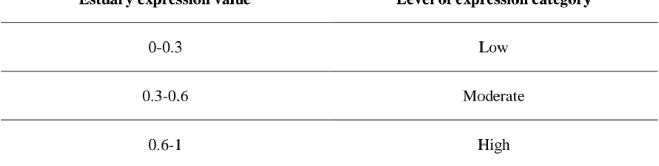
For each primary symptom, an area weighted expression value for each zone is determined, and the symptom level of expression S1 was then obtained by summation.
n e z E A A S 1 1 1 (Eq. 14)Where Az is the surface area of each zone; Ae is the total estuarine surface area; E1 is
the expression value at each zone; n is the number of estuarine zones.
The level of expression of the primary symptoms for the estuary P1 is determined
by calculating the average of two primary symptom expression values and estuary is then assigned a category for primary symptoms according to Table 18.
Table 18 Categories for primary and secondary symptoms.
Estuary expression value Level of expression category
0-0.3 Low
0.3-0.6 Moderate
0.6-1 High
3.7.2.2. Secondary symptoms method (SSM)
and nuisance and toxic blooms), an area weighted expression value for each zone is determined as described above. The level of expression of secondary symptoms for the estuary is determined by choosing the highest of the three estuary level symptom expression values. Secondary symptoms are considered to be a clear indicator of problems, and the application of the precautionary principle means that the highest (worst-case) value dictates the classification. The estuary is then assigned a category for secondary symptoms according to Table 17.
3.7.2.3. Overall ranking of eutrophic conditions
Finally, the primary and secondary symptoms are compared in a matrix to determine an overall level of eutrophic conditions for the estuary. As shown in Fig. 5, OEC is derived from a combination of Y-Axis (Primary symptoms) with X-Axis (Secondary symptoms).
(adapted from Bricker et al., 2003).
3.7.3. Pressure--Overall Human Influence (OHI)
The basic assumption for OHI is that different systems vary in responding to any particular level of nutrient input, due to varying levels of susceptibility to nutrient inputs (Bricker et al., 1999). And thus, it is determined by combining system susceptibility and nutrient inputs.
3.7.3.1. Nutrient load
This section is to determine the nutrient inputs being delivered to the water body from human activities. The watershed estimates are provided for five major nutrient source types: point sources, fertilizer, livestock, atmospheric deposition, and non-point/non-agricultural.
To simplify the complexity in coastal exchange, only conservative (mixing) processes are considered to derive the nutrient component of OHI. A simple ―Vollenweider‖ mass balance model is used to describe the dispersive exchange between an estuarine black box and the ocean (Ferreira, 2000; Bricker et al., 2003).
out in w M M dt dM (Eq. 15) where Mw is the mass of nutrient in the estuary; Min is nutrient loading to the
estuary (kg s-1); Mout is nutrient discharge from the estuary (kg s-1).
Human-derived nutrient concentration mh is derived as following equation:
s s m m e in h 1 (Eq. 16)
where min is the nitrogen concentration in the inflow (kg m-3); se is mean estuarine
salinity (no unit); Δs is the difference between offshore salinity and mean estuary salinity.
The calculation of background nutrient concentration mb is:
o e sea b s s m m (Eq. 17)
where msea is nitrogen concentration from the sea (kg m-3); so is offshore salinity.
The overall human influence (OHI) then may be obtained from Eq. 16 and 17:
h b h m m m OHI (Eq. 18) The ratio derived describes the comparison of nutrients from watershed or land based (human) loads with oceanic or natural loads. It determines the categorical response (Table 19), which is afterwards used to combine with the categorical response for susceptibility (Bricker et al., 2003).
Table 19 Thresholds set categories used to classify overall human influence (adapted from Bricker
et al., 2003).
Class Thresholds Score
Low 0 to <0.2 5
Moderate low >0.2 to 0.4 4
Moderate >0.4 to 0.6 3
Moderate high >0.6 to 0.8 2
3.7.3.2. Susceptibility
Susceptibility is defined as the relative capacity of a system to dilute and/or flush nutrients.
Dilution potential is determined as a function of the system volume, weighted with a stratification term. Flushing potential is a relative to tidal range and river flow.
By combining dilution and flushing components, an export potential is determined (Fig. 6).
Fig.6. Combination of dilution and flushing for
susceptibility (adapted from Bricker et al., 2003).
3.7.3.3. Determination of the overall level of human influence
OHI is determined by comparing susceptibility to retain nutrients with the level of nutrient input, as shown in following matrix (Fig. 7).
Fig.7. Combination of susceptibility and nutrient input for OHI (adapted from Bricker et al.,
2003).
3.7.4. Response--Determination of Future Outlook (DFO)
DFO is performed to determine the likelihood of whether conditions in an estuary will worsen, improve, or stay the same over the next twenty years. Assessment of expected changes in nutrient pressures are carried out based on a variety of drivers, including demographic trends, wastewater treatment and remediation plans, and changes in watershed uses. Since the state of estuarine system is related not only to the nutrient pressures, but also to system carrying capacity, there is a need to include aforementioned susceptibility. Therefore, projection of future nutrient inputs is combined, in this section, with system susceptibility to obtain a foreseeable evolution (Fig. 8).
Fig.8. Combination of susceptibility and future nutrient pressure for DFO (adapted from Bricker et
al., 2003).
3.7.5. Synthesis--Overall grade
The last stage of ASSETS is to synthesize the three indices mentioned above to provide an overall description of system status in terms of eutrophication. The combination of individual classifications for pressure, state and response is able to provide a grade falling into one of five categories: high, good, moderate, poor or bad (Table 20). Since there are five grades for each component, theoretically allows 53 possibilities. However, clearly not every aggregation makes sense, and thus 31 highly improbable or unreasonable combinations were excluded.
Table 20 Combination of pressure (OHI), state (OEC) and response (DFO) components to provide
an overall grade (adapted after Bricker et al., 2003).
These five categories are used by the EU Water Framework Directive (EUWFD, 2000/60/EC). Although the Directive is designed for EU members, the framework provides a useful scale for setting eutrophication-related reference conditions for different types of systems (Bricker et al., 2006).
Chapter 4. Discussion of methodology
In this section, the different methods are discussed and compared in terms of the rationale behind them. ―Phase I‖ approaches usually establish nutrient-based classification systems through the measurement of variables such as transparency, nutrients and chlorophyll a, while ―Phase II‖ approaches look at the symptoms. The details of comparisons are presented as follows.
4.1. Comparison among “Phase I” and “Phase II” methods
Even though the nutrient index methods aforementioned are the recommended approach by Chinese national authority, they have been criticized for their underlying simplicity and limitation (Yao & Shen, 2005). The main reasons that the ―Phase I‖ methods are considered not appropriate in assessing Chinese coastal systems lie on: a. They overemphasize the significance of nutrient concentration as an indicator of
eutrophication, which instead may not be a robust diagnostic variable. Nutrients are the primary cause, but there are many factors causing or responding to the increase of eutrophic level, such as the presence of nuisance and loss of submerged vegetation. High concentrations are not necessarily indicative of eutrophication, and low concentrations do not inevitably guarantee the absence of eutrophication (Cloern, 2001; Dettmann, 2001; Bricker et al., 2003).
b. These freshwater-based methods fail to adapt themselves to coastal systems due to the unawareness of the difference between freshwater and coastal systems. It has been recognized in the last decades that estuarine and coastal eutrophication is