www.atmos-chem-phys.net/16/71/2016/ doi:10.5194/acp-16-71-2016
© Author(s) 2016. CC Attribution 3.0 License.
A comprehensive inventory of ship traffic exhaust emissions in the
European sea areas in 2011
J.-P. Jalkanen, L. Johansson, and J. Kukkonen
Finnish Meterological Institute, P.O. Box 503, 00101 Helsinki, Finland
Correspondence to:J.-P. Jalkanen (jukka-pekka.jalkanen@fmi.fi)
Received: 19 December 2014 – Published in Atmos. Chem. Phys. Discuss.: 11 March 2015 Revised: 30 November 2015 – Accepted: 14 December 2015 – Published: 14 January 2016
Abstract. Emissions originating from ship traffic in Euro-pean sea areas were modelled using the Ship Traffic Emis-sion Assessment Model (STEAM), which uses Automatic Identification System data to describe ship traffic activity. We have estimated the emissions from ship traffic in the whole of Europe in 2011. We report the emission totals, the sea-sonal variation, the geographical distribution of emissions, and their disaggregation between various ship types and flag states. The total ship emissions of CO2, NOx, SOx, CO, and
PM2.5in Europe for year 2011 were estimated to be 121, 3.0,
1.2, 0.2, and 0.2 million tons, respectively. The emissions of CO2 from the Baltic Sea were evaluated to be more than a
half (55 %) of the emissions of the North Sea shipping; the combined contribution of these two sea regions was almost as high (88 %) as the total emissions from ships in the Mediter-ranean. As expected, the shipping emissions of SOx were
significantly lower in the SOxEmission Control Areas,
com-pared with the corresponding values in the Mediterranean. Shipping in the Mediterranean Sea is responsible for 40 and 49 % of the European ship emitted CO2and SOxemissions,
respectively. In particular, this study reported significantly smaller emissions of NOx, SOx, and CO for shipping in the
Mediterranean than the EMEP inventory; however, the re-ported PM2.5emissions were in a fairly good agreement with
the corresponding values reported by EMEP. The vessels reg-istered to all EU member states are responsible for 55 % of the total CO2emitted by ships in the study area. The vessels
under the flags of convenience were responsible for 25 % of the total CO2emissions.
1 Introduction
The cornerstone of air quality modelling research is an up-to-date description of emissions from all sectors of an-thropogenic (i.e. industry, agriculture, transport) and non-anthropogenic (i.e biogenic, desert dust, wildland fires) ac-tivities. However, information on emissions may have lim-ited dynamical features, such as the geographical or tempo-ral variations of emissions. This is especially important for transport emissions, which vary substantially both spatially and temporally.
Determination of shipping activity has previously been one of the largest unknowns in assessing the emissions from the maritime transport sector. The traffic activities of ship-ping in Europe are nowadays well known, as compared with vehicular traffic; this was not the case previously. The intro-duction of automatic vessel position reporting systems, such as the Automatic Identification System (AIS), have signifi-cantly reduced the uncertainty concerning ship activities and their geographical distribution. Nowadays, all vessels larger than the 300 t size limit globally report their position with a few second intervals; this has resulted in an availability of in-formation on ship activities at an unprecedented level of de-tail. The ship emission inventories, which are based on such automated identification systems, have several significant ad-vantages over the previously developed approaches. Such in-ventories are based on time-dependent, high-resolution dy-namic traffic patterns, which can also allow for the effects of changing conditions, such as, e.g. marine and meteorological conditions (e.g. harsh winter conditions and sea ice cover) or weather routing.
al., 2002), voluntary weather reports from ships (ICOADS, Corbett et al., 2007) or search and rescue services (AMVER, Endresen et al., 2003; Wang et al., 2008). None of these data sources is able to reflect the total ship activity with full flex-ibility of traffic activity and temporal changes. Inconsisten-cies can exist between geographical emission inventories and satellite observations of pollutants (Vinken et al., 2014). Fur-thermore, important emission sources, like ships in harbours have been often neglected from regional emission studies.
The availability of the shipping activity data for research can be a challenging task; however, there are several options for data acquisition. Data collected by maritime authorities are rarely available for research purposes. However, there are networks of volunteers maintaining AIS base stations; activity data can therefore either be shared or are commer-cially available. Most satellite AIS data sets are available from commercial service providers, but also national space programs may provide access to these. Automatic AIS data collection facilitates annually updated ship emissions in the EU waters; however, the coverage area should be expanded to the Northeast Atlantic Ocean. This could be done with the inclusion of other activity data sources, such as, e.g. the satel-lite AIS data, which could be used to extend the AIS cover-age, e.g. to fully cover the EMEP modelling domain.
In this work, we present emissions for European sea re-gions, which are covered by the terrestrial network of AIS base stations. In general, European seas are relatively densely trafficked, especially in regions in which intercontinental ship traffic intersects with busy short sea shipping routes. The vessel activity data from this area have been collected at the operational Vessel Traffic Services centre at the European Maritime Safety Agency. This centralized data archive al-lows one of the most comprehensive high-resolution sources of vessel activity on a continental scale. The modelling ap-proach of the present study can be largely automated, which facilitates annual updates of large-scale ship emissions. This allows, e.g for the inclusion of the impacts of policy changes, such as sulphur reductions, to be included in the emission in-ventories used in air quality applications.
We have used the Ship Traffic Emission Assessment Model (Jalkanen et al., 2009, 2012; Johansson et al., 2013) which combines the vessel activity (AIS data) with vessel-specific information of main and auxiliary engines. This al-lows the determination of vessel-specific emissions, which are based on the detailed technical information of fuel-consuming systems onboard. Fuel type used during harbour stays or open seas will be determined from actual vessel ac-tivity and engine characteristics taking possible sulphur re-strictions in specific regions into account. The fuel type as-signment (residuals/distillates) is determined from technical specifications of ships’ engines which can provide a more realistic description of the use of various marine fuels than fleet-wide adoption of residual fuels.
The aim of this study is to present a comprehensive inven-tory of ship traffic exhaust emissions for a number of
con-taminants (CO2, NOx, SOx, PM2.5, CO) in European sea
ar-eas, utilizing the STEAM ship emission model (Jalkanen et al., 2009, 2012; Johansson, 2013). A more specific aim is to geographically present and discuss the high-resolution spa-tial distributions of shipping emissions for selected species, and the shares of emissions in terms of the various ship types and flag states. We have also identified the 30 highest emis-sion intensities in the European sea and harbour areas; these regions contain the highest amounts of predicted shipping emissions of CO2within a radius of 10 km. We aim also to
compare the numerical values of this new emission inven-tory with the corresponding values presented in some previ-ous inventories on the emissions originated from European shipping.
2 Materials and methods
2.1 Geographical domain and input data sets
This modelling approach uses as input values the position re-ports generated by the automatic identification system (AIS); this system is globally on-board in every vessel that weighs more than 300 t. The AIS system provides automatic updates of the vessel positions and instantaneous speeds of ships at intervals of a few seconds. For this paper, we used the AIS messages received by the terrestrial AIS network and pro-vided by the European Maritime Safety Agency (EMSA). We extracted the data that corresponded to the year 2011; the data contained more than 109 archived AIS messages. The
data have been collected from the terrestrial AIS base sta-tion network of the EU member states. The coverage of this network is illustrated in Fig. 1.
Most of the European sea areas are well represented in these data. However, the Arctic Ocean has not been included. Extensive open-sea areas, such as the Atlantic Ocean, are also not completely represented, due to the limited reception range of the terrestrial AIS base station network. There are also spatial gaps of the data in the southernmost parts of the Mediterranean, especially near the northern African coast-line. The data did not include position reports from any of the African countries; however, the ship activity in this area is significantly lower than in the northern parts of the Mediter-ranean. This was shown with an independent investigation of satellite AIS data sets obtained from the Norwegian Coastal Administration (detailed results not shown here). The data from inland waterways in Europe have been included, but cannot be taken to fully reflect the inland shipping, as the IMO SOLAS regulation does not require the use of AIS from these vessels.
Figure 1.The geographical coverage of the terrestrial AIS network in Europe. The colour scale illustrates the number of position reports per unit area, received in the EU sea areas in 2011.
IHS Fairplay (IHS, 2014) was the most significant source. The technical data were supplemented with material from several other companies and agencies. These included the following: Det Norske Veritas, Nippon Kaiji Kyokai, Bureau Veritas, Germanischer Lloyd American Bureau of Shipping, publicly available ship registers (such as the Korean, Nor-wegian, and Russian ship registers), ship owners and engine manufacturers. Fuel type was determined based on the prop-erties of engines, such as power output, angular velocity and stroke type. The sulphur content was assigned based on the current regulations in European sea areas, such as the MAR-POL Annex VI (IMO, 2008) and the EU Sulphur Directive.
The technical specifications were collected and archived for more than 65 000 vessels that have an International Mar-itime Organization (IMO) number. This set of ships repre-sents a majority of the global commercial fleet. In addition to these vessels, the AIS position reports were received from more than 35 500 vessels, for which the technical data could not be determined based on the information from classifica-tion societies, such as the Lloyds Register. In addiclassifica-tion to the
IMO number, the vessel Maritime Mobile Service Identity (MMSI) code was used as a secondary key in searching ves-sel data from ship databases.
However, the vessel data were not received for a vast ma-jority of vessels that transmitted the MMSI code (and no IMO number) in AIS data. An additional attempt to iden-tify these vessels with internet search engines using MMSI code was made for 5000 vessels, which had the largest fuel consumption. This revealed some potentially large vessels, but the impact of this step on overall CO2emissions was just
over one percent. Clearly, the default method of assuming those vessels small, which do not transmit IMO registry num-ber, introduces uncertainty to overall results, but the impact is negligible.
2.2 The STEAM model and its application
et al. (2009, 2012) and Johansson et al. (2013). This study does not introduce any refinement of the model.
The STEAM model was used to combine the AIS-based information with the detailed technical knowledge of the ships. This combined information is used to predict vessel water resistance and instantaneous engine power of main and auxiliary engines. The model predicts as output both the instantaneous fuel consumption and the emissions of se-lected pollutants. The fuel consumption and emissions are computed separately for each vessel, by using archived re-gional scale AIS data results in a rere-gional emission inventory. The STEAM emission model allows for the influences of the high-resolution travel routes and ship speeds, engine load, fuel sulfur content, multi-engine set-ups, abatement methods and the effects of waves (Jalkanen et al., 2012; Johansson et al., 2013).
The STEAM model includes a possibility to model some environmental effects on ships, such as the effects of waves and the influence of sea currents. However, for simplicity these factors were not taken into account in this study. The waves increase fuel consumption and emissions, whereas the direct effects of the wind and sea currents can be negative or positive. In considering long timescales and extensive re-gions, the net influences of direct wind effects and sea cur-rents are expected to be fairly small. It would be possible also to use satellite-based AIS messages as input values of the model; however, for simplicity these were not used in this study, except for the above-mentioned confirmation of lack of significant vessel activity in the southern Mediterranean Sea.
The emissions of NOx were modelled as a function of
crankshaft angular velocity (revolutions per minute, rpm), according to the IMO Tier I and II rules (IMO, 2008). Tier I rule was applied also to those ships that were built be-fore 2000; this assumption can result in a slight underestima-tion of emissions originated from these vessels. The effects of emission abatement techniques were also modelled, and certified emission factors have been used whenever possible. The emission certificates were provided by a group of ship owners, the emissions of these vessels had been measured by an accredited laboratory, in order to obtain a discount in the system of Swedish fairway dues. However, the vessels that were equipped with emission abatement techniques or had been subject to certified emissions represented less than 1 % of the ships included in this study.
We have included in the modelling most of the various engine setups, such as gas turbines, diesel electric and me-chanical power transmission, nuclear vessels and sailboats. We allowed for the fact that the operation of a shaft gen-erator is possible for vessels, which have been indicated to have geared drives or power take-off systems. The modelled values of engine loads also take into account multi-engine setups and load balancing of operational engines.
The STEAM model simulates the required power of the main and auxiliary engines by determining the required
power level set up that corresponds to the speed value in the AIS messages. All ships are modelled individually, and the modelling takes into account the differences in hull form, propeller efficiency, shaft generators and auxiliary engine us-age. The sulphur content of the fuel has been modelled ex-plicitly for each vessel and its engines. We have allowed for the sulphur reduction techniques and the influences of the regulations regarding fuel sulphur content in various regions and during various time periods (Johansson et al., 2013).
In cases, in which more detailed information could not be obtained from engine manufacturers, the Specific Fuel Oil Consumption (SFOC) has been modelled based on the meth-ods in the second IMO GHG report (Buhaug et al., 2009). The SFOC is modelled as a function of engine load. In the model, low engine load levels can increase SFOC up to 25 %. Operating engines outside their optimal working range (with-out de-rating) will lead to increased SFOC and emission fac-tors. The emissions of particulate matter, sulphate and water are modelled as a function of the fuel sulphur content. All vessels have been treated as single displacement hulls; cata-marans and hydrofoil vessels were not separately modelled. The currently modelled pollutants are NOx, SOx, CO, CO2,
EC, OC, ash, and hydrated SO4. The model can also be used
to generate vessel-specific emission inventories, and to pre-dict the amount of consumed fuel. The transport work (cargo payload) is described as the product of the weight of cargo transported and the distance travelled (commonly in units of ton km). In this work we adopted the scheme reported by the second IMO GHG study (Buhaug et al., 2009).
Detection of locations with the highest shipping emissions of CO2
We have evaluated in more detail the emissions from lo-cations with an especially high emission intensity, which we refer to as shipping emission “hotspots”. The STEAM model has been executed on a resolution of approximately 2.5 km×2.5 km in the EU region. For the evaluation of hotspots the resulting CO2 emission grid has subsequently
been evaluated using the following rules:
1. The sum of emissions in the vicinity of each grid cell has been calculated within a radius of 10 km (such a domain contains approximately 44 closest grid cells). 2. The sum (if high enough) along with centre coordinates
are placed in the list of top 30 highest ranking CO2
hotspots.
3. The first and second steps are repeated until each cell in the emission grid has been once the candidate emission hotspot.
Table 1.Emissions and shipping statistics in the SafeSeaNet area in 2011. The section “All ships” includes also emissions from unidentified vessels. “IMO registered” refers to commercial ships with specified IMO number. In the section “GT”, eight vessel size categories and their contributions to emitted CO2are presented. The NOxemissions have been calculated as NO2and SOxas SO2.
EU – 2011 CO2 NOx SOx PM2.5 CO Payload Ships Travel (t) (t) (t) (t) (t) (109t×km) (106km)
All 120 722 000 2 964 300 1 208 000 181 600 197 000 10 540 47 233 889 IMO 118 709 900 2 930 900 1 201 500 179 900 194 100 10 540 27 728 827 Unidentified 2 012 100 33 300 6500 1600 2800 0 19 505 61
Region Mediterranean Sea 48 344 100 1 228 600 594 800 82 900 77 400 4400 – 288 Atlantic Ocean 19 276 900 511 200 272 600 36 600 32 900 2349 – 124 North Sea 20 736 000 477 400 108 200 22 100 35 800 1463 – 190 Baltic Sea 15 004 000 328 800 83 900 16 200 21 500 864 – 128 English Channel 6 699 900 171 700 40 200 7700 10 800 677 – 47 Irish & British Seas 4 975 500 121 900 59 000 8200 8000 421 – 41 Norwegian Sea 2 399 200 49 500 17 900 2900 4000 104 – 35 Black Sea 1 305 700 32 600 14 100 2000 2400 145 – 15 Bay of Biscay 865 800 19 300 8600 1200 1400 56 – 9
Inland 790 400 15 600 5300 900 1600 40 – 10
Red Sea 224 400 5200 2300 300 400 21 – 1
Ship types Container ship 34 089 400 924 300 414 000 59 200 67 600 3440 1213 131 Tanker 26 145 600 668 000 273 500 41 000 38 400 3616 2879 160 Cargo ship 20 078 800 508 600 208 800 30 400 34 500 2887 5220 285 RoPaX 16 956 700 359 900 127 700 21 000 20 000 122 9884 74 Vehicle carrier 9 427 900 229 700 99 300 14 400 13 200 475 961 56 Cruise ship 5 004 800 107 200 43 500 6700 6500 0 253 14 Other 3 012 500 57 200 15 000 3000 6000 0 4002 43 Service vessel 2 036 100 39 200 8700 1900 3600 0 866 15 Fishing vessel 1 381 800 26 000 7200 1300 2900 0 1829 33 Passenger ferry 576 000 10 400 3500 600 900 0 621 15
GT (GT < 4000 t) 14 496 600 272 700 72 000 14 000 25 700 395 31 770 359 (4000 t < GT < 10 000 t) 15 092 900 330 000 114 800 18 700 24 500 758 4042 161 (10 000 t < GT < 20 000 t) 15 018 800 376 000 146 000 21 800 24 000 968 2814 100 (20 000 t < GT < 30 000 t) 18 822 100 478 400 195 800 29 000 27 400 1573 2668 95 (30 000 t < GT < 45 000 t) 16 536 800 436 200 181 000 26 500 25 200 1664 2548 68 (45 000 t < GT < 60 000 t) 10 878 200 289 100 123 400 18 000 17 100 1137 1060 37 (60 000 t < GT < 80 000 t) 10 127 000 278 400 120 500 17 400 18 500 1301 855 28 (GT > 80 000 t) 19 749 300 503 100 254 200 35 700 34 200 2745 1476 40
3 Results and discussion
3.1 Summaries of total emissions and their geographical distribution in Europe
A compilation of computed emissions, payloads, numbers of ships, and distances travelled has been presented in Ta-ble 1. The geographical distribution of ship CO2emissions
and hotspots and are illustrated in Figs. 2 and 3. The re-sults have been presented in terms of (i) IMO registered and unidentified ships, (ii) sea regions, (iii) top flag states, and (iv) ship types. The percentages of the total ship emissions in each of the sea regions for the selected pollutants have also been presented graphically in Fig. 4. The region denoted as “other” (that refers to other European sea areas) includes the western parts of the Black Sea, Canary Islands, Celtic Sea, Barents Sea and Northeast Atlantic Ocean (see Fig. 1).
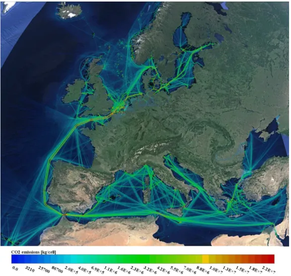
The highest CO2 emissions are located along the
bus-iest shipping lines near the coast of the Netherlands and in the English Channel, in the straits of Gibraltar, Sicily and Bosporus, and in the Danish Straits. In addition, there are localized high amounts of CO2 emissions near several
major ports. These ports include, in particular, the ones in the Netherlands (e.g. Antwerp, Rotterdam, and Amsterdam), Gibraltar, St. Petersburg, and some ports in the UK, Ger-many, Italy, and Spain. The relative geographical distribution of the shipping emissions is similar also for the other mod-elled compounds, and those results have therefore not been presented here.
Figure 2.Predicted geographic distribution of shipping emissions of CO2in Europe in 2011. The colour code indicates emissions in relative mass units per unit area.
via shorter routes. For example, there are a lot of routes be-tween the islands in Greece and the mainland, and bebe-tween Italy and the islands of Sardinia, Corsica, and Sicily. There is a dense network of shorter passenger vessel routes in nu-merous sea regions in the Mediterranean. The routes of cargo and passenger traffic intersect also in several regions of the Baltic Sea and the North Sea. For example, in the English Channel passenger traffic takes place mainly across the chan-nel, whereas most of the cargo routes are aligned along the Channel.
We have also analysed the areas that have the highest CO2
shipping emissions in Europe. These areas were defined as circular domains with a radius of 10 km. We have presented the results for 30 areas that had the highest estimated emis-sions. These domains are called in the following text as the emission hot spots. The results have been presented in Ta-ble 2 and in Fig. 3. The combined CO2 emissions of these
30 hotspot areas correspond to approximately 7 % of total CO2emitted by ships in Europe.
The area including the Netherlands and the English Chan-nel has the highest density of these hot spots; there are in total 10 domains in these regions amongst the top 30 ship-ping CO2hotspots in Europe. There are also hot spots at
nu-merous locations in the Mediterranean, some in Germany, and a few in the Baltic Sea region. Harbour areas dominate the list of highest CO2hotspots. Besides harbour locations,
some shipping lanes and some major coastal cities are asso-ciated with very high CO2emissions. Clearly, a major part
of emissions in these coastal cities are also due to harbour activities. Several of the largest harbours in Europe reside in the Netherlands and along the English Channel.
In some sea regions, busy shipping traffic is focused in ge-ographical bottlenecks with high CO2emissions; prominent
Figure 3.The 30 locations in which there were highest ship emissions of CO2in Europe in 2011. The area of each circle is proportional to the annual CO2emission.
study. The data from Greece and Romania include part of vessel activity from this area, but not a sufficient coverage.
Emissions of CO2 originated from Mediterranean
ship-ping were found to be about 40 % of the total CO2emissions
from shipping. Emissions from ships in the North Sea and the Baltic Sea constituted approximately one quarter and one eight of the total emissions of CO2 from shipping,
respec-tively. The emissions of NOxfrom the ships in the
Mediter-ranean Sea (1 229 000 t, calculated as NO2) are almost as
high as those in the Baltic Sea (329 000 t) and the North Sea (649 000 t) combined. The emissions of NOxfrom other
areas considered in this study are slightly higher than the contribution from the North Sea shipping. The share of the Mediterranean Sea traffic is even larger in case of the SOx emissions, compared with the corresponding emissions for CO2and NOx.
The emissions originated from the other sea areas except for the three specifically mentioned three sea regions (Baltic Sea, North Sea and Mediterranean Sea) have also been re-ported in Table 1 and Fig. 4. These areas include the western parts of the Black Sea, Canary Islands, Celtic Sea, Barents Sea and Northeast Atlantic Ocean. The emissions from ship-ping in these other regions were estimated to produce almost one quarter of CO2; however, this value is probably an
un-derestimation, as the coverage of AIS reception in remote sea areas, such as the Atlantic Ocean, is incomplete. It is also likely that inland shipping is only partially covered in our analysis.
Figure 4.The fractions of shipping emissions for European sea re-gions in 2011.
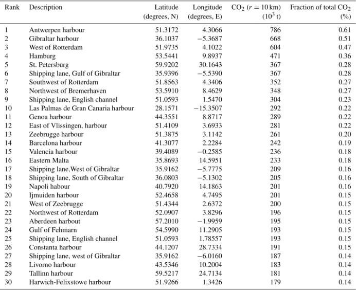
Table 2.The locations in European sea areas that contain the highest CO2emissions within a circular area that has a radius of 10 km.
Rank Description Latitude Longitude CO2(r=10 km) Fraction of total CO2
(degrees, N) (degrees, E) (103t) (%)
1 Antwerpen harbour 51.3172 4.3066 786 0.61
2 Gibraltar harbour 36.1037 −5.3687 668 0.51
3 West of Rotterdam 51.9735 4.1022 604 0.47
4 Hamburg 53.5441 9.8937 471 0.36
5 St. Petersburg 59.9202 30.1643 367 0.28
6 Shipping lane, Gulf of Gibraltar 35.9396 −5.5390 367 0.28
7 Southwest of Rotterdam 51.8563 4.3406 352 0.27
8 Northwest of Bremerhaven 53.5910 8.4629 348 0.27
9 Shipping lane, English channel 51.0593 1.5470 304 0.23
10 Las Palmas de Gran Canaria harbour 28.1571 −15.3507 292 0.22
11 Genoa harbour 44.3551 8.8717 289 0.22
12 East of Vlissingen, harbour 51.4109 3.6933 281 0.22
13 Zeebrugge harbour 51.3875 3.1142 261 0.20
14 Barcelona harbour 41.3077 2.2284 242 0.19
15 Valencia harbour 39.4089 −0.2585 236 0.18
16 Eastern Malta 35.8693 14.5951 233 0.18
17 Shipping lane,West of Gibraltar 35.9162 −5.7775 209 0.16
18 Shipping lane, South of Gibraltar 36.0803 −5.1302 205 0.16
19 Napoli habour 40.7920 14.1863 201 0.16
20 Ijmuiden harbour 52.4658 4.7495 201 0.15
21 West of Zeebrugge 51.4344 2.6372 200 0.15
22 Northwest of Rotterdam 52.0907 3.8296 196 0.15
23 Aberdeen harbout 57.2010 −1.9959 195 0.15
24 Gulf of Fehmarn 54.5990 11.2905 193 0.15
25 Shipping lane, English channel 51.0593 1.78557 193 0.15
26 Constanta harbour 44.1207 28.7334 191 0.15
27 Shipping lane, west of Gibraltar 35.9162 −6.0160 187 0.14
28 Livorno harbour 43.5346 10.2004 183 0.14
29 Tallinn harbour 59.5217 24.7134 181 0.14
30 Harwich-Felixstowe harbour 51.9266 1.3426 179 0.14
emission hot spots, especially those which are in the vicinity of major cities, are prime candidates for enhanced emission control measures. The low fuel sulphur requirement of the EU directive has already addressed some aspects of this is-sue.
3.2 Analysis of emissions in terms of the flag state and the ship type
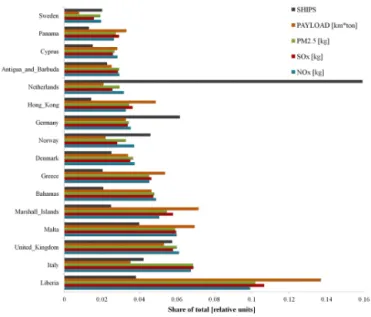
The AIS signals include a Maritime Mobile Service Iden-tity (MMSI) code that contains information that specifies the flag state of the ship. We have selected 16 flag states that had the highest total fuel consumption in Europe in 2011, and evaluated their annual statistics of the numbers of ships, pay-load, and the emissions of three pollutants. The results of this analysis are included in Fig. 5. The emissions have been pre-sented as fractions (%) of the total emissions in the European sea areas in Fig. 5.
The emissions were largest for the Liberian and sec-ond largest for the Italian fleet. The UK, Malta, Ba-hamas, Norway, and the Netherlands also have had
ma-jor fleets. In addition to mama-jor European states, such as Italy, UK, Norway, the Netherlands, Greece, Germany, etc., major fleets have also sailed under the flags of rel-atively smaller states, such as Liberia, Malta, Bahamas, Marshall Islands, etc. The flags of convenience allow open vessel registration regardless of the owner’s na-tionality (ITF, http://www.itfglobal.org/en/transport-sectors/ seafarers/in-focus/flags-of-convenience-campaign/), which is in contrast with national ship registries. The states among the top 16 fuel consumers with the flags of convenience are Panama, Cyprus, Antigua and Barbuda, Marshall Islands, Bahamas, Malta, and Liberia. The CO2 emission shares of
vessels in open registries are responsible for 25 %, European vessels contribute 55 % and vessels with some other flag con-tribute 20 % of the total CO2emissions. The emissions
Figure 5.Relative contributions of various flag states to selected emissions, the numbers of ships and cargo payload in Europe in 2011. We have selected 20 states that had the highest emissions of CO2. These states have been presented in terms of the emissions of CO2; the lowest entry (Liberia) in the figure had the highest emis-sions.
We have allocated the emissions to IMO registered (re-ferred here also as “large”) and unidentified (re(re-ferred to as “small”) ships in Table 1, as the IMO registered ships con-stitute most of the commercial marine traffic. According to the values in Table 1, the contribution of unidentified ves-sels is only 1.7 % of the total CO2emissions, although the
number of such small vessels is over 41 % of all vessels. The unidentified ships travel 7 % of the distances travelled by all vessels. For some countries, such as the Netherlands, Germany, France, and Sweden, the share of large vessels is less than one third of the total number of ships. This may indicate the different practices in including the small vessel movements in overall traffic image of various countries. It is very likely that small vessel traffic is underestimated by AIS, because for these vessels AIS is voluntary, in contrast to the requirements for large vessels. In this context, the Dutch fleet is an extreme case, in which only 13 % of 7530 ves-sels are considered large. In the Dutch case, the share of CO2
emitted by small vessels is 43 %, which is the largest frac-tion for all of the studied fleets. The large number of small vessels in the AIS data in the case of the Dutch fleet can be explained by the fact that the use of the AIS equipment is compulsory in the non-recreational inland vessels in the Netherlands. In Finland, there are over 190 000 motor boats (Trafi, 2014) and 525 Finnish vessels were picked up by AIS in Europe. Clearly, the representation of small vessel traffic substantially varies between countries; their activities are in-completely represented in the AIS signals.
Figure 6.The fractions of European shipping emissions and pay-load, classified in terms of the ship types, in 2011.
The descriptions of the technical details for small vessels in the emission inventory are limited. These are significantly less accurate than the corresponding descriptions for large vessels, for which the engine setup and technical data are readily available. Model results for the fuel consumption of small vessels are further complicated by an incomplete inclu-sion of the activities of small vessels; a fraction of the small vessels do not carry AIS equipment on board.
The shares of emissions for various ship types have been presented in Fig. 6. A comparison of CO2emissions and
pay-load reflects the energy efficiency of various ship types. We used the approach described by Buhaug et al. (2009). The unit emissions (the mass of CO2emitted, divided by
trans-port work) are lowest for the tanker class (7.3 g t−1km−1), slightly higher for container (10.2 g t−1km−1) and cargo ves-sels (10 g t−1km−1), and significantly higher for passenger traffic (175 g t−1km−1). However, the values for passenger traffic are not directly comparable, as the above-mentioned transport work of passenger traffic has been calculated as a function of cargo capacity, which does not take the number of passengers into account. There are large variations of unit emissions between various vessels in the cargo class, as this class includes both dry bulk and palletized cargo vessels, for which there are large differences in the use of their cargo car-rying capacity.
3.3 Seasonal variation of the emissions
There were clear seasonal variations in the emissions of all pollutants; the variations in case of CO2have been presented
in Fig. 7. For example, the emissions of CO2in June are 30 %
Figure 7.Seasonal variation of the shipping emissions of CO2in the European sea regions in 2011, classified in terms of various ves-sel categories.
summer months (June, July, and August), both the numbers of passenger vessels and small vessels is the largest, espe-cially in the Mediterranean Sea. This is mainly caused by the increased recreational travel; in summer the number of small vessels is at a maximum in all sea areas. The emissions of container ships are also higher in the summer than winter, but the activities of tankers and cargo ships exhibit no sub-stantial seasonal dependency. Recently, Ialongo et al. (2014) used satellite-based OMI NOx observations to track the
an-nual variability of NOxemissions from Baltic Sea shipping.
Ialongo et al. demonstrated a decrease in satellite-observed NOx similar to Jalkanen et al. (2014). Although the
emis-sions cannot be directly compared with observations of at-mospheric columns of NOx, decrease of NOx was observed
in both data sets which coincide with the economic downturn during 2008–2009.
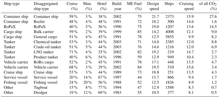
A disaggregated compilation of vessel types and their op-erational features has been presented in Table 3. The five more general level categories (cargo, container, tanker, pas-senger, and other) have been divided into more detailed cat-egories. The division of vessel activity to operational modes (cruising, maneuvering, and hotelling) has not been predeter-mined; it has been defined by vessel activity data. Based on AIS data, it is possible to determine these explicitly, which will significantly decrease the large uncertainties that have previously been associated with vessel activities.
The shares of fuel used by the main engines have also been presented in Table 3, these have also been evaluated by the model. The amounts of fuel used in main and auxil-iary engines depend not only on vessel specifics, but also its operational profile. However, there is a major uncertainty in the predictions of the fuel consumption of the auxiliary en-gine, as the use of an auxiliary engine varies greatly, even for ships of the same type. The use of auxiliary power can-not be determined from tank tests of ship resistance, unlike the power needed for propulsion, for which various theo-ries exist for performance prediction. In this study, we have
used the methodology presented previously (Jalkanen et al., 2009, 2012; Johansson et al., 2013). This method combines the information on cargo capacity, auxiliary engine power profiles, main and auxiliary engine setup and power trans-mission method. However, there are also other modelling ap-proaches, which are based on extensive vessel boarding pro-grams (Starcrest, 2013), local knowledge, and pre-assigned contributions (Dalsøren et al., 2009). The share of auxiliary engine fuel consumption from total consumption is very high for service vessels and tugboats. This is consistent with the 2nd IMO GHG report by Buhaug et al. (2009); however, the contribution of these vessels to the total fuel consumption or CO2emission from shipping in the study area is small, less
than 2.5 %.
3.4 Comparison of the predictions of various emission inventories
The comparison of the numerical results of various European-scale emission inventories can be challenging, as pointed out, e.g. by EEA (2013). The main reasons for this are that the methodologies and various modelling selections used for evaluating shipping emissions vary substantially in various published studies. E.g. the various studies may de-fine differently the geographical domain, and some studies address only international ship traffic.
The current work reports emissions for the year 2011. Sig-nificant reductions were therefore in force regarding the sul-phur content of marine fuel in the North Sea and the Baltic Sea area, as well as the requirement for low sulphur fuel in EU harbour areas. The effects of these regulations were included in the current work, and it is therefore not possi-ble to directly compare the predicted SOx and PM2.5
emis-sions with the corresponding values during previous years. Changes in international regulations also concern NOx, but
to a lesser extent, as the IMO Tier II NOxlimits for marine
diesel engines affect all engines built since 1 January 2011. The ships constructed after this date will have to conform to Tier II NOxrequirements (15 % less NOxproduced when
compared with Tier I engines), but such new ships constitute only 3 % of the fleet of IMO registered vessels in this study. Significant policy changes are expected to be implemented in 2015, regarding the sulphur content of marine fuel.
The emissions of NOx for the Mediterranean Sea
re-ported in this work are lower than in the EMEP inventory; qualitatively the same conclusion was reported by Marmer et al. (2009). Marmer et al. (2009) also concluded that their methodology yielded lower SOx emissions than the
corresponding EMEP values. The prediction of the STEAM inventory for the Mediterranean shipping in the case of NOx
Table 3.Summary of average operational features of some selected ship types. The first column indicates the aggregated ship type, whereas the second column contains a more detailed description of vessel type. The time spent in each operation mode (cruising, maneuvering, hotelling) is indicated by the next three columns as percentages. “ME of Fuel” refers to the fraction of fuel used in main engines from total fuel consumption. Cruising speed indicates average cruising speed observed in AIS data. The last column on the right-hand side indicates the significance of contribution to overall CO2emissions. These ship types are responsible for over 98 % of total CO2emitted.
Ship type Disaggregated Cruise Man. Hotel Build ME Fuel Design Ships Cruising of all CO2
ship type (%) (%) (%) year (%) speed speed (%)
Container ship Container ship 59 % 3 % 38 % 2002 75 21.7 2373 15.9 27.6
Container ship Reefer 48 % 4 % 48 % 1991 72 18.2 500 14.6 1.6
RoPaX RoPaX 40 % 5 % 56 % 1990 75 19.0 1207 13.6 14.5
Cargo ship Bulk carrier 59 % 2 % 39 % 1999 85 14.2 4008 12.1 9.0
Cargo ship General cargo 51 % 4 % 45 % 1991 78 12.5 5855 9.9 8.2
Tanker Chemical tanker 53 % 3 % 44 % 2003 71 14.0 2385 12.0 8.8
Tanker Crude-oil tanker 51 % 5 % 44 % 2003 76 14.6 1216 12.0 6.9
Tanker LNG tanker 71 % 4 % 25 % 2002 82 19.2 219 14.7 2.7
Tanker Product tanker 40 % 6 % 54 % 1996 59 12.9 949 10.4 2.3
Vehicle carrier RoRo cargo 52 % 2 % 45 % 1991 78 17.1 448 13.5 4.7
Vehicle carrier Vehicle carrier 68 % 3 % 29 % 2002 84 19.5 510 15.6 3.4
Cruise ship Cruise ship 53 % 3 % 44 % 1989 73 18.8 251 13.5 4.3
Service vessel Service vessel 20 % 14 % 67 % 1997 44 13.7 866 9.4 1.7
Fishing vessel Fishing vessel 24 % 20 % 56 % 1988 52 12.5 1826 8.9 1.2
Other Tugboat 15 % 8 % 77 % 1994 47 12.9 1588 8.3 0.7
Other Dredger 19 % 12 % 69 % 1983 55 10.5 377 8.1 0.5
the OMI instrument to constrain top-down emissions from ships. The study area of this study (defined by AIS coverage illustrated in Fig. 1) and Vinken et al. (2014) are the same (N, W, S boundaries are same), except that the domain used by Vinken et al. (2014) extends further to the East (50◦E); neither of these assessments includes the trans-Atlantic ship traffic.
The reported total NOxemission for all European sea areas
in our study is 2.96 million t, which corresponds to 0.9 mil-lion t of reduced nitrogen (N). This is close to the correspond-ing value reported by Vinken et al. (2014), their estimate for European shipping emissions was 1.0 million t of reduced ni-trogen for the year 2006. Unfortunately, AIS data from 2005– 2006 for all European sea areas are not available since at the time AIS had just been deployed as a navigational aid and fleet-wide adoption of AIS was in progress. The difference between the NOxemissions of the STEAM and EMEP
inven-tories in the Baltic Sea shipping is 18 % (the emission values of STEAM is higher). However, the comparison with Vinken et al. (2014) is challenging for the Baltic Sea, as Vinken et al. (2014) report only emissions along the major ship tracks, which are not representative of the emissions in the whole of the Baltic Sea area.
The annual SOx emissions reported in this study for
var-ious sea regions are 84 000, 148 000, and 595 000 t for the Baltic Sea, North Sea/English Channel, and the Mediter-ranean, respectively. The corresponding SOx emissions of
the EMEP inventory for the above-mentioned sea areas are 69 000, 163 000, and 978 000 t, taking into account the up-date of the EMEP inventory in 2015. For the Baltic Sea and
the North Sea, the inventories are approximately in agree-ment (their differences are 22 and 10 %), but there is a larger difference in the predicted emissions of SOx in the Mediter-ranean Sea. The SOx emissions predicted in this study for
the Mediterranean are about two thirds of the corresponding values in the EMEP inventory.
The reasons for such major differences in the predictions of these two inventories could be caused, for example, by the neglect of the impacts of relevant legislation, such as the EU sulphur directive (EU, 2012). This directive limits the sulphur content of marine fuels to 0.1 % (by mass) in har-bour areas and to 1.5 % (by mass) for passenger vessels on a regular schedule. It is possible that not all passenger ships comply with the requirement of 1.5 % fuel sulphur content, as assumed in the STEAM model. However, a possible non-compliance by a fairly small fraction of ships would explain only a minor portion of the differences between the STEAM and EMEP inventories. More information on the compli-ance with EU regulations can be obtained either during Port State Control checks, or via relevant compliance monitoring schemes (Balzani et al., 2014; Berg et al., 2012; Beecken et al., 2014, 2015; Pirjola et al., 2014).
Plotting the EMEP time series of SOx and NOx for the
shipping in the Mediterranean indicate that the NOx and
SOxemissions decreased in a similar way during 2007–2010,
probably reflecting the overall decreases in both shipping and economic activity. However, between 2009 and 2010, the SOxemissions in EMEP inventories increased by more than
6 %, whereas the corresponding NOx emissions from ships
directive came into force in January 2010, with requirements for the reduction of marine fuel sulphur content. This would have been expected to decrease the SOxemissions from the
shipping in the Mediterranean, instead of increasing them. However, in 2010 the new NOx limits (IMO Tier II) were
implemented for vessels constructed since 2010, but in 2011 only 3 % of the fleet were new ships. Calculating backwards from SO2values of Table 1, the average fuel sulphur content
(denoted here byS) of some major ship types yields 1.9 %S for container ships, 1.6 % Sfor tankers, 1.2 %S for RoPax and 1.4 %Sfor cruise vessels. It should be noted that these values represent a combination of SOx from both main and
auxiliary engines, which may use fuels with different fuel sulphur content. Also, these averages include contributions from vessels sailing both the SECA and the non-SECA’s. The differences in the STEAM and EMEP inventories war-rant further study; these differences should also be examined using dispersion modelling and air quality measurements.
It is not possible to perform a similar satellite-based com-parison for SOx, due to the technical limitations of currently
available satellite instruments; these cannot accurately de-termine ship emitted SOxnear the sea surface. Such
instru-ments can detect stationary SO2sources that have an
emis-sion higher than approximately 70 kt (Fioletov et al., 2013); however, this value is too high for the shipping lanes in Eu-rope.
The inventory of Cofala et al. (2007) includes an esti-mate for ship CO2 emissions, which is based on the same
methodology as the EMEP inventories. According to Co-fala et al. (2007), the predicted CO2emission in 2010 from
ships in the Mediterranean is approximately 76 million t (ob-tained by a linear interpolation between the values in 2000 and 2020), whereas in this work, the Mediterranean shipping was responsible for 48 million t of CO2emitted.
The differences in PM2.5emissions between this work and
Cofala et al. (2007) in all sea areas are less than 20 %. A large variation could be expected in the PM2.5emissions
pre-dicted by the various methods, due to the substantial vari-ability of experimentally determined emission factors and the differences in PM2.5sampling methods (e.g. Jalkanen et al.,
2012). Clearly, the PM2.5emissions are associated with the
SOxemissions and the sulphur content of the fuel, as SO4is
one of the main constituents of atmospheric PM2.5.
The range of European shipping emissions of CO2
re-ported in the review by EEA (2013) is 71–153 million t (for various years between 2000–2009), based on the work of EEA (2013), Cofala et al. (2007), Whall et al. (2002), Sch-rooten et al. (2009) and Campling et al. (2012); the estimate of the present study is at the higher end of this range. Simi-larly, in case of NOxemissions, the range of values in
vari-ous inventories reviewed by EEA (2013) is 1.7–3.6 million t whereas this study evaluated the European emissions from shipping in 2011 to be 2.94 million t, calculated as NO2.
However, in case of NOx the inclusion of variability in
as-sumptions of technology development (Tier I, II, inclusion
of NOxabatement, NOxemission factor rpm dependency) of
marine engines can have a large impact on overall NOx
re-sults of various inventories, especially if ship emissions from different years are compared.
4 Conclusions
The comparison of emitted pollutants with existing ship emission inventories revealed that there are some differences between the estimates of the various inventories for the emis-sions of ships sailing the Mediterranean Sea, whereas the results were better in agreement for the North Sea and the Baltic Sea regions. The NOx, SOx, and CO emissions
evalu-ated in this study for the Mediterranean Sea were 18, 39, and 49 % lower than the corresponding values in the EMEP and IIASA inventories. The PM2.5emissions from the STEAM
inventory were 24 % lower than indicated by the EMEP emis-sion inventory. Satellite observations using the Ozone Moni-toring Instrument (OMI) also indicated smaller annual emis-sions of NOxin the Mediterranean, compared with the
pre-dictions of the EMEP inventory. These differences should be investigated further with a longer ship emission time series, which takes into account the relevant changes of the envi-ronmental legislation. From a technical point of view, it is feasible to have annual updates of bottom-up ship emission inventories.
Further research is required including emission modelling in combination with consecutive chemical transport mod-elling, comparisons with measured atmospheric concentra-tions of pollutants and source apportionment. The reasons for these deviations between different emission inventories should be investigated further and confirmed with indepen-dent experimental data sets, as these can have significant pol-icy implications concerning health and environmental impact assessments within the transport sector. A logical step would be to include chemical transport modelling and comparisons with air quality measurements especially at coastal stations to determine whether the predicted NOxand SOx
concentra-tions are in an agreement with the measurements.
Despite the wide geographical extent, the ship emission data can also be segmented in terms of the various proper-ties of vessel categories or individual vessels. This makes it possible to classify the emissions using several criteria. The disaggregation of ship emissions into individual vessels on a fine temporal resolution also allows fine resolution air qual-ity and health impact assessment studies. A specific advan-tage of an inventory based on individual vessel data is that it facilitates comparisons with experimental stack measure-ments.
According to this study, the vessels carrying an EU flag were responsible for 55 % of CO2 emissions in the EU,
whereas the states with flags of convenience and other states constitute the remaining share. The CO2hotspot mapping
ship emitted CO2, both from harbour areas and densely
traf-ficked shipping lanes.
The emissions from ships have a clear seasonal variation; the emission maximum occurs during the summer months. This concerns especially passenger traffic, but also container-ships have the same seasonal pattern. However, the emissions originated from oil tankers and other cargo ships do not have a clear seasonality. Temporal variation of ship emissions has mostly been neglected in previous emission inventories, due to inherent limitations of the activity data used as a basis for these inventories. Seasonal variations can be of the order of 30 %; these features should therefore be included in emission and health impact assessments.
The current work also facilitates studies of ship energy ef-ficiency, as all emissions and fuel data are generated on the ship level. There were substantial differences between fuel burned and transport work carried out by various ship types. The unit emissions were the lowest for the oil tankers and largest for passenger vessels. However, the description of transport work of passenger vessels currently considers cargo operations and does not completely cover passenger cargoes.
Data availability
The gridded emission data sets of this work can be made available for further research upon request to the authors.
Acknowledgements. This study was made possible as a result of
cooperation with the European Maritime Safety Agency and the Norwegian Coastal Administration. We would like to thank both agencies for making the relevant AIS data sets available for this work. We are also grateful for financial support of the European Space Agency (Samba project), FP7 project TRANSPHORM and the Academy of Finland (APTA project). This work is partly based on the material supplied by IHS Fairplay.
Edited by: W. Birmili
References
Balzani Lööv, J. M., Alfoldy, B., Gast, L. F. L., Hjorth, J., Lagler, F., Mellqvist, J., Beecken, J., Berg, N., Duyzer, J., Westrate, H., Swart, D. P. J., Berkhout, A. J. C., Jalkanen, J.-P., Prata, A. J., van der Hoff, G. R., and Borowiak, A.: Field test of available meth-ods to measure remotely SOxand NOxemissions from ships,
At-mos. Meas. Tech., 7, 2597–2613, doi:10.5194/amt-7-2597-2014, 2014.
Beecken, J., Mellqvist, J., Salo, K., Ekholm, J., and Jalkanen, J.-P.: Airborne emission measurements of SO2, NOxand particles
from individual ships using a sniffer technique, Atmos. Meas. Tech., 7, 1957–1968, doi:10.5194/amt-7-1957-2014, 2014. Beecken, J., Mellqvist, J., Salo, K., Ekholm, J., Jalkanen, J.-P.,
Jo-hansson, L., Litvinenko, V., Volodin, K., and Frank-Kamenetsky, D. A.: Emission factors of SO2, NOx and particles from ships
in Neva Bay from ground-based and helicopter-borne measure-ments and AIS-based modeling, Atmos. Chem. Phys., 15, 5229– 5241, doi:10.5194/acp-15-5229-2015, 2015.
Berg, N., Mellqvist, J., Jalkanen, J.-P., and Balzani, J.: Ship emis-sions of SO2and NO2: DOAS measurements from airborne plat-forms, Atmos. Meas. Tech., 5, 1085–1098, doi:10.5194/amt-5-1085-2012, 2012.
Bosch, P., Coenen, P., Fridell, E., Åström, S., Palmer, T., and Hol-land, M.: Cost Benefit Analysis to support the impact assessment accompanying the revision of Directive 1999/32/EC on the sul-phur content of certain liquid fuels, AEA Technology, European Commission reports ENV.C.5/FRA/2006/0071, Harwell, Didcot OX, UK, 2009.
Brandt, J., Silver, J. D., Christensen, J. H., Andersen, M. S., Bøn-løkke, J. H., Sigsgaard, T., Geels, C., Gross, A., Hansen, A. B., Hansen, K. M., Hedegaard, G. B., Kaas, E., and Frohn, L. M.: Assessment of past, present and future health-cost externalities of air pollution in Europe and the contribution from international ship traffic using the EVA model system, Atmos. Chem. Phys., 13, 7747–7764, doi:10.5194/acp-13-7747-2013, 2013.
Buhaug, Ø., Corbett, J. J., Endresen, Ø., Eyring, V., Faber, J., Hanayama, S., Lee, D. S., Lee, D., Lindstad, H., Markowska, A. Z., Mjelde, A., Nelissen, D., Nilsen, J., Palsson, C., Winebrake, J. J., Wu, W.-Q., and Yoshida, K.: Second IMO GHG study, In-ternational Maritime Organization (IMO), London, UK, 2009. Campling, P., Janssen, L., and Vanherle, K.: Specific evaluation of
emissions from shipping including assessment for the establish-ment of possible new emission control areas in European Seas, VITO, Mol, Belgium, 2012.
Cofala, J., Amann, M., Heyes, C., Wagner, F., Klimont, Z., Posch, M., Schöpp, W., Tarasson, L., Jonson, J. E., Whall, C., and Stavrakaki, A.: Analysis of Policy Measures to Reduce Ship Emissions in the Context of the Revision of the National Emissions Ceilings Directive – Final Report. Contract number 070501/2005/419589/MAR/C1, International Institute for Ap-plied Systems Analysis, Vienna, Austria, 2007.
Corbett, J. J., Winebrake, J. J., Green, E. H., Kasiblathe, P., Eyring, V., and Lauer, A.: Mortality from Ship Emissions: A Global As-sessment, Environ. Sci. Technol., 41, 8512–8518, 2007. Dalsøren, S. B., Eide, M. S., Endresen, Ø., Mjelde, A., Gravir, G.,
and Isaksen, I. S. A.: Update on emissions and environmental im-pacts from the international fleet of ships: the contribution from major ship types and ports, Atmos. Chem. Phys., 9, 2171–2194, doi:10.5194/acp-9-2171-2009, 2009.
EEA: The impact of international shipping on European air quality and climate forcing, EEA Technical report No 4/2013, Copen-hagen, Denmark, 2013.
Endresen, Ø., Sørgård, E., Sundet, J. K., Dalsøren, S. B., Isaksen, I. S. A., Berglen, T. F., and Gravir, G.: Emission from international sea transportation and environmental impact, J. Geophys. Res., 108, 4560, doi:10.1029/2002JD002898, 2003.
EU: Directive 2012/33/EU of the European Parliament and of the Council of 21 November 2012 amending Council Directive 1999/32/EC as regards the sulphur content of marine fuels, Stras-bourg, France, 2012.
detection of large emission sources, J. Geophys. Res.-Atmos., 118, 11399–11418, 2013.
Ialongo, I., Hakkarainen, J., Hyttinen, N., Jalkanen, J.-P., Johans-son, L., Boersma, K. F., Krotkov, N., and Tamminen, J.: Charac-terization of OMI tropospheric NO2over the Baltic Sea region, Atmos. Chem. Phys., 14, 7795–7805, doi:10.5194/acp-14-7795-2014, 2014.
IHS Global: Chemin de la Mairie, Perly, Geneva, Switzerland, 2014.
International Maritime Organization (IMO): Regulations for the prevention of air pollution from ships and NOxtechnical code,
Annex VI of the MARPOL convention 73/78, London, UK, Oc-tober 2008.
Jalkanen, J.-P., Brink, A., Kalli, J., Pettersson, H., Kukkonen, J., and Stipa, T.: A modelling system for the exhaust emissions of marine traffic and its application in the Baltic Sea area, At-mos. Chem. Phys., 9, 9209–9223, doi:10.5194/acp-9-9209-2009, 2009.
Jalkanen, J.-P., Johansson, L., Kukkonen, J., Brink, A., Kalli, J., and Stipa, T.: Extension of an assessment model of ship traffic exhaust emissions for particulate matter and carbon monoxide, Atmos. Chem. Phys., 12, 2641–2659, doi:10.5194/acp-12-2641-2012, 2012.
Jalkanen, J.-P., Johansson, L., and Kukkonen, J.: A Comprehensive Inventory of the Ship Traffic Exhaust Emissions in the Baltic Sea from 2006 to 2009, Ambio, 43, 311–324, 2014.
Johansson, L., Jalkanen, J.-P., Kalli, J., and Kukkonen, J.: The evo-lution of shipping emissions and the costs of regulation changes in the northern EU area, Atmos. Chem. Phys., 13, 11375–11389, doi:10.5194/acp-13-11375-2013, 2013.
Jonson, J. E., Jalkanen, J. P., Johansson, L., Gauss, M., and De-nier van der Gon, H. A. C.: Model calculations of the effects of present and future emissions of air pollutants from shipping in the Baltic Sea and the North Sea, Atmos. Chem. Phys., 15, 783– 798, doi:10.5194/acp-15-783-2015, 2015.
Kalli, J., Jalkanen, J.-P., Johansson, L., and Repka, S.: Atmospheric emissions of European SECA shipping: long-term projections, WMU J. Marit. Affairs, 12, 129–145, 2013.
Marmer, E., Dentener, F., Aardenne, J. V., Cavalli, F., Vignati, E., Velchev, K., Hjorth, J., Boersma, F., Vinken, G., Mihalopoulos, N., and Raes, F.: What can we learn about ship emission invento-ries from measurements of air pollutants over the Mediterranean Sea?, Atmos. Chem. Phys., 9, 6815–6831, doi:10.5194/acp-9-6815-2009, 2009.
Pirjola, L., Pajunoja, A., Walden, J., Jalkanen, J.-P., Rönkkö, T., Kousa, A., and Koskentalo, T.: Mobile measurements of ship emissions in two harbour areas in Finland, Atmos. Meas. Tech., 7, 149–161, doi:10.5194/amt-7-149-2014, 2014.
Schrooten, L., De Vlieger, I., Int Panis, L., Chiffi, C., and Pastori, E.: Emissions of maritime transport: A European reference system, Sci. Total Environ., 408, 318–323, 2009.
Starcrest: Port of Los Angeles Inventory of Air Emissions 2012, 2013.
Trafi: Finnish Transport Safety Agency, National small boat regis-ter, available at: http://www.veneily.fi/venerekisteri, last access: 24 November 2014.
USEPA: Regulatory impact analysis control of emissions of air pol-lution from locomotive engines and marine compression ignition engines less than 30 liters per cylinder, EPA/OTAQ, Washington DC, USA, 2008.
Vinken, G. C. M., Boersma, K. F., van Donkelaar, A., and Zhang, L.: Constraints on ship NOxemissions in Europe using
GEOS-Chem and OMI satellite NO2observations, Atmos. Chem. Phys., 14, 1353–1369, doi:10.5194/acp-14-1353-2014, 2014.
Wang, C., Corbett, J. J., and Firestone, J.: Improving Spatial Rep-resentation of Global Ship Emissions Inventories, Environ. Sci. Technol., 42, 193–199, 2008.