ISSN 1549-3644
© 2010 Science Publications
Corresponding Author: Abdo Abou Jaoude, Department of Applied Mathematics,
Aix-Marseille University, France and the Lebanese University, Lebanon
116
Prediction in Complex Dimension Using Kolmogorov’s Set of Axioms
1
Abdo Abou Jaoude,
2Khaled El-Tawil and
3Seifedine Kadry
1Department of Applied Mathematics, Aix-Marseille University,
France and the Lebanese University, Lebanon
2
Departement of Civil Engineering, Faculty of Engineering,
Lebanese University, Campus of Hadath, Lebanon
3Departement of Computer Science, Faculty of Sciences,
Lebanese University, Campus of Zahle, Lebanon
Abstract: Problem statement: The five basic axioms of Kolmogorov define the probability in the real set of numbers and do not take into consideration the imaginary part which takes place in the complex set of numbers, a problem that we are facing in many engineering systems. Approach: Evaluate the complex probabilities by considering supplementary new imaginary dimensions to the event occurring in the “real” laboratory. The Kolmogorov’s system of axioms can be extended to encompass the imaginary set of numbers and this by adding to the original five axioms of Kolmogorov an additional three axioms. Hence, any experiment can thus be executed in what is now the complex set C which is the sum of the real set R with its corresponding real probability and the imaginary set M with its corresponding imaginary probability. Results: Whatever the probability distribution of the random variable in R is, the corresponding probability in the whole set C is always one, so the outcome of the random experiment in C can be predicted totally. Conclusion: The result indicated that, the chance and luck in R is replaced now by total determinism in C. This is the consequence of the fact that the probability in C is got by subtracting the chaotic factor from the degree of our knowledge of the system.
Key words: Kolmogorov’s axioms, random variable, probability, real set, imaginary set, complex set, complex number, probability norm, degree of knowledge of the system, chaotic factor, Bernoulli experiment, binomial distribution, Gaussian or normal distribution, density function, Young’s modulus
INTRODUCTION
Original Kolmogorov’s set of axioms: The simplicity of Kolmogorov’s system of axioms may be surprising. Let E be a collection of elements {E1, E2,…} called elementary events and let F be a set of subsets of E called random events. The five axioms for a finite set E (Benton, 1966; Montgomery and George, 2003; Walpole et al., 2002; Bell, 1992) are:
• F is a field of sets
• F contains the set E
• A non-negative real number Prob (A), called the probability of A, is assigned to each set A in F
• Prob (E) equal 1
• If A and B have no elements in common, the number assigned to their union is Prob (A∪B) = Prob
(A) + Prob (B); Hence, we say that A and B are disjoint; Otherwise, we have Prob (A∪B) = Prob (A) + Prob (B) – Prob (A∩B)
And we say also that Prob (A∩B) = Prob (A) × Prob (B|A) = Prob (B) × Prob (A|B) which is the conditional probability. If both A and B are independent, then Prob (A∩B) = Prob (A) × Prob (B). An example of probability would be the game of coin tossing. Let P1 denote the probability of getting head H and P2 denote the probability of getting tail T. Then we have:
E = {H,T}
F ={Φ,{H},{T},{H,T}}
117 Prob ({H} and {T}) = 0
And this according to the original Kolmogorov’s set of axioms.
ADDING THE IMAGINARY PART M
Now, if we can add to this system of axioms an imaginary part such that:
• Let Pm = i (1-Pr) be the probability of an associated event in M (the imaginary part) to the event A in R (the real part). It follows that Pr + Pm/i = 1 where i2 = -1 (the imaginary number)
• We construct the complex number Z = Pr + Pm = Pr + i(1-Pr) having a norm | Z |2=Pr2+(P / i)m 2
• Let Pc denote the probability of an event in the universe C where C = R + M. We say that Pc is the probability of an event A in R with its associated
event in M such that:
2 2 2
r m r m
Pc =(P +P / i) =| Z | −2iP P and is always equal to 1
We can see that the system of axioms defined by Kolmogorov could be hence expanded to take into consideration the set of imaginary probabilities (Abou Jaoude Abdo, 2004; 2005; 2007).
Example 1: Coin tossing (Bernoulli experiment): If we return to the game of coin tossing, we define the probabilities as follows:
Output R M
Getting Head Pr1=p1 Pm1=q1 = i (1–p1)
Getting Tail Pr2=p2 Pm2=q2 = i (1–p2)
Sum i
i
p =1
∑
ii
q =i
∑
If we calculate 2 1
| Z | for the event of getting Head, we get:
2 2 2
1 1 1
2 2 2 2
1 1 1 1
1 1 1 1
| Z | Pr (Pm / i)
p (q / i) p (1 p )
1 2p (p 1) 1 2p (1 p )
= +
= + = + −
= + − = − −
This implies that:
2 2 2
1 1 1 1 1 1 1 1 1
2 2 2 2
1 1 1 1 1 1 1
1 | Z | 2p (1 p ) | Z | 2.i.p .i(1 p ) | Z | 2i Pr Pm
Pr (Pm / i) 2i Pr Pm (Pr Pm / i) Pc
= + − = − − = −
= + − = + =
where, i2 = i × i = -1 and 1 i i= − .
This is coherent with the axioms already defined and especially axiom 8. Similarly, if we calculate 2
2|
Z |
for the event of getting Tail, we get:
2 2 2
2 2 2
2 2 2 2
2 2 2 2
2 2 2 2
| Z | Pr (Pm / i)
p (q / i) p (1 p )
1 2p (p 1) 1 2p (1 p )
= +
= + = + −
= + − = − −
This implies that:
2 2 2
2 2 2 2 2 2 2 2 2
2 2 2 2
2 2 2 2 2 2 2
1 | Z | 2p (1 p ) | Z | 2.i.p .i(1 p ) | Z | 2i Pr Pm
Pr (Pm / i) 2i Pr Pm (Pr Pm / i) Pc
= + − = − − = −
= + − = + =
This is also coherent with the axioms already defined and especially axiom 8.
ROLE OF THE IMAGINARY PART
It is apparent from the set of axioms that the addition of an imaginary part to the real event makes the probability of the event in C always equal to 1. In fact, if we begin to see the universe as divided into two parts, one real and the other imaginary, understanding will follow directly. The event of tossing a coin and of getting a head occurs in R (in our real laboratory), its correspondent probability is Pr. One may ask directly what makes that we ignore the output of the experiment (e.g., tossing the coin). Why should we use the probability concept and would not be able to determine surely the output? After reflection one may answer that: if we can know all the forces acting upon the coin and determine them precisely at each instant, we can calculate their resultant which will act upon the coin, according to the well known laws of dynamics and determine thus the output of the experiment:
i i
F =ma
∑
where: F = The force m = The mass a = The acceleration
118 the simple experiments of dynamics like of a falling apple or a rolling body experiments where the hidden variables are totally known and determined and which are: Gravitation, air resistance, friction and resistance of the material. But when the hidden variables become difficult to determine totally like in the example of lottery-where the ball has to be chosen mechanically by the machine in an urn of hundred moving bodies!!!-we are not able in the latter case to determine precisely which ball will be chosen since the number of forces acting on each ball are so numerous that the kinematics study is very difficult indeed. Consequently, the action of hidden variables on the coin or the ball makes the result what it is. Hence the complete knowledge of the set of hidden variables makes the event deterministic; That is, it will occur surely and thus the probability becomes equal to one, (Boursin, 1986; Dacunha-Castelle, 1996; Dahan et al., 1992; Ekeland, 1991; Gleick, 1997; Kuhn, 1970; Poincare, 1968; Prigogine, 1997; Prigogine and Isabelle, 1992; Dahan and Peiffer, 1986).
Now, let M be the universe of the hidden variables and let 2
| Z | be the degree of our knowledge of this phenomenon. Pr is always and according to Kolmogorov’s axioms, the probability of an event. A total ignorance of the set of variables in M makes:
• Pr = Prob (getting Head) = 1/2 and Prob (getting Tail) = 1/2 (if they are equiprobable)
• 2
1
| Z | in this case is equal to
1 1
1 2p (1 p )− − = − ×1 (2 1 / 2) (1 1 / 2)× − =1 / 2
Conversely, a total knowledge of the set in R makes: Prob (getting Head) = 1 and Pm = Prob (imaginary part) = 0. Therefore, we have 2
1
| Z | = − × × − =1 (2 1) (1 1) 1
because the phenomenon is totally known, that is, its laws are determined; hence, our degree of our knowledge of the system is 1 or 100%.
Now, if we can tell for sure that an event will never occur i.e. like ‘getting nothing’ (the empty set), in the game of Head and Tail, Pr is accordingly = 0, that is the event will never occur in R. Pm will be equal to i(1-Pr) = i(1-0) = i and 2
1
| Z | = − × × −1 (2 0) (1 0)= 1, because we can tell that the event of getting nothing surely will never occur thus our degree of knowledge of the system is 1 or 100%.
It follows that we have always: 1 / 2≤ Z2≤1 since
2 2 2
r m
Z =P +(P / i) and 0≤P , Pr m≤1. And in all cases we
have: 2 2 2
r m r m
Pc =(P+P / i) = Z −2iP P =1.
Meaning of the last relation: According to an experimenter tossing the coin in R, the game is a game of luck: the experimenter doesn’t know the output in the sense already explained. He will assign to each outcome a probability Pr and say that the output is not deterministic. But in the universe C = R + M, an observer will be able to predict the outcome of the game since he takes into consideration the contribution of M, so we write:
2 2
r m
Pc =(P +P / i)
So in C, all the hidden variables are known and this leads to a deterministic experiment executed in an eight dimensional universe (four real and four imaginary; where three for space and one for time in R and three for space and one for time in M) (Balibar, 1980; Greene, 2000; 2004; Hoffmann et al., 1975). Hence Pc is always equal to 1. In fact, the addition of new dimensions to our experiment resulted to the abolition of ignorance and non-determination. Consequently, the study of this class of phenomena in C is of great usefulness since we will be able to predict with certainty the outcome of experiments conducted. In fact, the study in R leads to non-predictability and uncertainty.
So instead of placing ourselves in R, we place ourselves in C then study the phenomena, because in C the contributions of M are taken into consideration and therefore a deterministic study of the phenomena becomes possible. Conversely, by taking into consideration the contribution of the hidden forces we place ourselves in C and by ignoring them we restrict our study to non-deterministic phenomena in R (Srinivasan and Mehata, 1988; Stewart, 1996; 2002; Van Kampen, 2006; Weinberg, 1992).
THE CHAOTIC FACTOR CHF
It follows from the above definitions and axioms that:
r m r r
2iP P = × × × −2i P i (1 P )=
2
r r r r
2i × × −P (1 P )= −2P (1 P )− =Chf
r m
2iP P will be called the chaotic factor in our experiment and is denoted by ‘Chf ‘. We will see why we have called this term the chaotic factor, in fact:
119
• In case Pr = 0, that is in the case of an impossible event:
Chf= -2×0× (1-0) = 0.
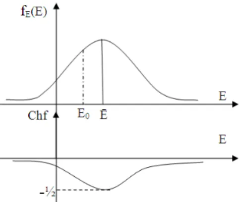
• In case Pr = 1/2, Chf = -2 × 1/2 × (1-1/2) = -1/2 We notice that −1 / 2≤Chf≤0 and hence,
2 2
Pc = Z −Chf . Then we can conclude that (Fig. 1): Pc2 = Degree of our knowledge of the system-chaotic
factor = 1 therefore Pc = 1
This means that if we succeed to eliminate the chaotic factor in an experiment, the output will always be with the probability = 1, (Gleick, 1997; Orluc and Herve, 2005; Ducrocq and Warusfel, 2004).
A moving body: If a set of forces is acting upon a body of mass m, the resultant law of dynamics would be:
i i
F=ma
∑
Where: F = The force m = The mass a = The acceleration
Fig.1: The graphs of |Z|2 and Chf in function of Pr
The second law of dynamics will enable us to determine the exact position of the body after a time t, in condition that the sum of all the forces is totally known. Suppose that: i
i
F =mg+ + +R F f
∑
, that isgravitation, reaction, the force of friction and an unknown force f, are acting on the body. We note that f, may be positive (with the motion) or negative (against the motion). One can see that the chaotic factor is due to f and when the Chf = 0 then the probability that the body will be in a calculated position at time t is equal to 1. The study could easily lead to a probabilistic study of the trajectory of the body when f is ignored and when it is a random variable (hence the Chf is different from zero). A good illustration of this is the study of perfect gases in thermodynamics, (Gleick, 1997; Stewart, 1996; 2002).
THE DEVELOPMENT OF TWO STATISTICAL DISTRIBUTIONS
We will develop below two statistical distributions which are the binomial distribution and the normal distribution to illustrate the use of imaginary probabilities. The binomial law is the following (Walpole et al., 2002):
Prob [event] = C p qKN k N k
−
where, k
N N k
N N!
C C
k
k!(N k)!
= = =
− .
It is the probability to get an event k times from N repeated experiments, like in the game of tossing a coin N times. This law is discrete by nature.
The continuous law that we will illustrate here is the Gauss-Laplace distribution or the normal distribution (Benton, 1966):
2
1 x
dF (x, t).dx .exp .dx
4Dt 4 Dt
−
= ρ =
π
Where:
(x, t)
ρ = The density function of diffusion D = The diffusion factor
x = The displacement of the particle t = The time of displacement
x = 0 = mean value of x
2Dt
σ = = The standard deviation
120 Laplace. This density function is the continuous form of the discrete binomial theory that we have mentioned.
All our study is to compute probabilities. The new idea is to add new dimensions to our experiment and this will make the work deterministic. In fact, the probability theory is a non-deterministic theory by nature; that means that the outcome of the events is due to luck. In adding new dimensions to the event, we make the work deterministic and hence the game of tossing a coin will have a certain outcome in the complex set C. It is of great importance that the game of luck becomes totally predictable since we will be totally knowledgeable to predict the outcome of statistical events that occur in nature like in thermodynamics. Therefore the work that should be done is to add the contributions of M that make the event in C = R + M deterministic. If this is found to be fruitful, then a new theory in statistical sciences will be elaborated and this to understand deterministically those phenomena that used to be random phenomena in R.
First distribution: The Binomial distribution: Getting Head k times from N trials (Montgomery and George, 2003):
R M
k k N k k k N
Pr =p =C p q − Pmk=i(1 Pr )− k =i(1 p )− k
Summation:
N N N
k k N k N N
k k N
k 0 k 0 k 0
Pr p C p q − (p q) 1 1
= = = = = = + = =
∑
∑
∑
and
N N N N N
k k k k
k 0 k 0 k 0 k 0 k 0
Pm i.(1 Pr ) i (1 Pr ) i 1 Pr
i.[(N 1) 1] iN
= = = = = = − = − = − = + − =
∑
∑
∑
∑ ∑
If we compute the norm of the complex number
k k k Pr Pm
Z = + we get:
2 2 2 2 2
k k k k k
k k k k
Z Pr (Pm / i) p (1 p )
1 2p (p 1) 1 2p (1 p )
= + = + − =
+ − = − −
This implies that:
2 2
k k k k k k
2 2 2
k k k k k k k
2 2
k k k k
1 Z 2p (1 p ) Z 2.i.p .i.(1 p )
Z 2.i.Pr .Pm Pr (Pm / i) 2.i.Pr .Pm
(Pr Pm / i) Pc Pc 1
= + − = − − =
− = + − =
+ = ⇒ =
This is coherent with the axioms that we have already defined.
Second distribution: The Gaussian distribution: To find the probability of an event following the normal distribution, we use the density function. We should have k
k
p =1
∑
, or in continuous form we should have the integration over the whole domain equal to 1 like in this way (Benton, 1966; Chen et al., 1997):1 Dt 4 Dt 4 1 dx . Dt 4 x exp Dt 4 1 dx . Dt 4 x exp Dt 4 1 t).dx x, ( dF 2 2 = π × π = − π = − π = ρ =
∫
∫
∫
∫
∞ + ∞ − +∞ ∞ − +∞ ∞ − +∞ ∞ −Now, the probability of finding the particle in the interval between −∞and L is:
L 2
rob L L
1 x
exp .dx P [x L] Pr p ;
4Dt 4 Dt −∞ − = ≤ = =
π
∫
and the associated probability in M is:
2
L L rob
L
1 x
Pm i.(1 Pr ) i.P [x L] i. .exp .dx
4Dt 4 Dt
+∞ −
= − = > =
π
∫
= i.Prob [to find the particle in the interval L and +∞] Now, if we compute the norm of the complex number ZL=PrL+PmL we get:
2 2 2 2 2
L L L L L
L L L L
Z Pr (Pm / i) p (1 p )
1 2p (p 1) 1 2p (1 p )
= + = + − =
+ − = − −
This implies that:
2 2 2
L L L L L L
2 2
L L L L L L
2 2
L L L L
2 2
L L L L
1 Z 2p (1 p ) Z 2.i .p .(1 p )
Z 2.i.p .i.(1 p ) Z 2.i.Pr .Pm
Pr (Pm / i) 2.i.Pr .Pm
(Pr Pm / i) Pc Pc 1
= + − = − − = − − = − = + − = + = ⇒ = where, L
L L L
L
Z Pr Pm (x, t).dx i. (x, t).dx;
+∞
−∞
= + = ρ
∫
+∫
ρwritten for short
∫
∫
+∞ ∞ − + = L L L i Z .
121
2 L
2 2 L
L L L
2 L
2 L
i.
Pc (Pr Pm / i)
i 1 1 +∞ −∞ +∞ +∞ −∞ −∞ = + = + = + = = =
∫
∫
∫
∫
∫
This is also coherent with the axioms already defined.
Now the chaotic factor is:
L
L L L
L
L L L
L
Chf 2.i.Pr .Pm 2.i i
2 2 1
+∞ −∞ +∞ −∞ −∞ −∞ = = × × × = − × × = − × × −
∫
∫
∫
∫
∫
∫
One can directly see that ChfL = 0 if L→ −∞or
L→ +∞, that means that we will not find the particle in no place or we will find always the particle somewhere respectively. Finally, we say that:
2 2
L L L L
Pc = Z −2.i.Pr .Pm =Degree of our
knowledge-Chaotic factor = 1
where, ZL is the norm of ZL that combines here both
the contributions of R and M; hence, we can notice that
L
Z is a complex number. It is the chaotic factor that makes the study of an event in R a random process. Hence, any event in C is deterministic. This is the advantage of working in C.
Example: Application to Young’s modulus (Khaled, 2002): Let E be the Young’s modulus in a material domain as it is shown in the Fig. 2 and we assume that it follows a Gaussian distribution. Let E be the mean value of E and is taken to be equal to 29575 Ksi. Let
E
σ be the standard deviation of E and is equal to 1507 Ksi. Let the coefficient of variation be
E 1507
c.v 0.051
E 29575
σ
= = ≅ .
Fig. 2: The Young’s modulus E in a material domain
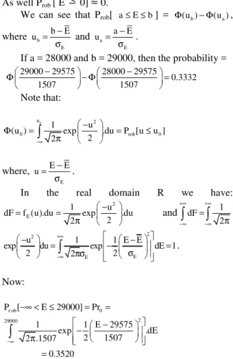
We can compute from the statistical tables that: Prob [28000 Ksi ≤E≤ 29000 Ksi] = 0.3332,
Prob [-∞<E≤29000 Ksi] = 0.3520 and Prob [29000 Ksi
≤E<+∞] = 0.6480 As well Prob [ E
≤
0]≈
0.We can see that Prob[ a≤ ≤E b] = Φ(u )b − Φ(u )a ,
where b E
b E
u = −
σ and a E
a E
u = −
σ .
If a = 28000 and b = 29000, then the probability =
29000 29575 28000 29575
0.3332
1507 1507
− −
Φ − Φ =
Note that: o
u 2
0 rob 0
1 u
(u ) exp .du P [u u ]
2 2
−∞
−
Φ = = ≤
π
∫
where,
E
E E
u= −
σ .
In the real domain R we have:
2 E
1 u
dF f (u).du exp .du
2 2
−
= =
π and
1 dF 2 +∞ +∞ −∞ −∞ = π
∫
∫
2 2 E Eu 1 1 E E
exp du exp dE 1
2 2 2
+∞ −∞ − − = − = σ
πσ
∫
.Now:
r ob 0
2 29000
P [ E 29000] Pr
1 1 E 29575
exp .dE
2 1507
2 .1507
0.3520 −∞
−∞ < ≤ = =
−
−
π
=
∫
The corresponding probability in the imaginary domain M is:
0 0 rob
2 29000
Pm i(1 Pr ) i.P [E 29000]
1 1 E 29575
i. exp .dE
2 1507
2 1507
i 0.6480 +∞
= − = > =
−
− =
π
×
∫
If we compute the norm of the complex number
0 0 0
Z =Pr+Pm we have:
2 2 2 2 2
0 0 0 0 0
0 0 0 0
Z Pr (Pm / i) Pr (1 Pr )
1 2 Pr (Pr 1) 1 2 Pr (1 Pr );
= + = + − =
122 This implies that:
2 2 2
0 0 0 0 0 0
2 2 2
0 0 0 0 0 0 0
2 2
0 0 0 0
1 Z 2 Pr (1 Pr ) Z 2.i .Pr .(1 Pr )
Z 2.i.Pr .Pm Pr (Pm / i) 2.i.Pr .Pm
(Pr Pm / i) Pc Pc 1
= + − = − − =
− = + − =
+ = ⇒ =
We note that:
0
0
0 0 0 E
E E
E
Z Pr Pm
f (u)du i f (u)du 0.3520 i 0.6480
+∞
−∞
= + =
+ = + ⋅
∫
∫
where E0=29000. We have also:
0
0
2 2
E
2 2 2
0 0 0
E
Pc (Pr Pm / i) 1 1
+∞ +∞
−∞ −∞
= + = + = = =
∫
∫
∫
And the chaotic factor is:
0 0 0
0
E E E
0 0 0
E
Chf 2.i.Pr .Pm 2.i i 2 1
+∞
−∞ −∞ −∞
= = × × × = − × × −
∫
∫
∫
∫
where, Chf0=0 if
= +∞
→
= −∞
→
1 Pr hence E
or
0 Pr hence E
0 0
0 0
.
Therefore, we say that:
2 2
0 0 0 0
Pc = Z −2.i.Pr .Pm =Degree of our
knowledge-Chaotic factor = 1. And if 2
0 0
Chf =0⇒| Z |=1, in other words, if the chaotic factor is zero, then the degree of our knowledge is 1 or 100%
Numerically, we write:
2 2 2
0
2
0 0 0
| Z | (0.3520) (0.6480)
0.123904 0.419904 0.543808
1
| Z | 0.737433 Chf 0, Notice that | Z | 1
2
= + =
+ = ⇒
= ⇒ ≠ ≤ ≤
Hence:
0
0
Chf 0.543808 1
1
0.456192, Notice that Chf 0
2
= − =
− − ≤ ≤
Fig. 3: The graphs of fE(E) and Chf in function of E Consequently, we can say that: The degree of our knowledge |Z0|
2
= 0.543808 and the chaotic factor Chf0 = −0.456192.What is interesting here is thus we have quantified both the degree of our knowledge and the chaotic factor of the event.
Notice that:
(
)
0
The degree of our knowledge 0.543808 – 0.456192
the chaotic factor 0.543808 0.456192 1 Pc
= −
− = + = =
Conversely, if we assume that:
2 2 2
0 0 0 0
Chf =0⇒| Z | =1⇒Pr +(Pm / i) =1
0 0
0 0
0 0
Pr 0 E
2 Pr (1 Pr ) 0 or or
Pr 1 E
= → −∞
⇒ − = ⇒ ⇒
= → +∞
2
0 0 0
1 1
Chf E E and | Z |
2 2
= − ⇒ = =
If E0increases to become=30,000 then both 2 0
| Z |
and Chf0 increase.
Therefore:
0
0 E
(Chf ) 0
lim
→+∞ = and 0
( )
2 0 E
Z 1
lim
→+∞ = where
2 2
0 0 0
Pc = Z −Chf =1, for every E0 in the real set R
(Fig. 3 and 4).
NUMERICAL SIMULATIONS
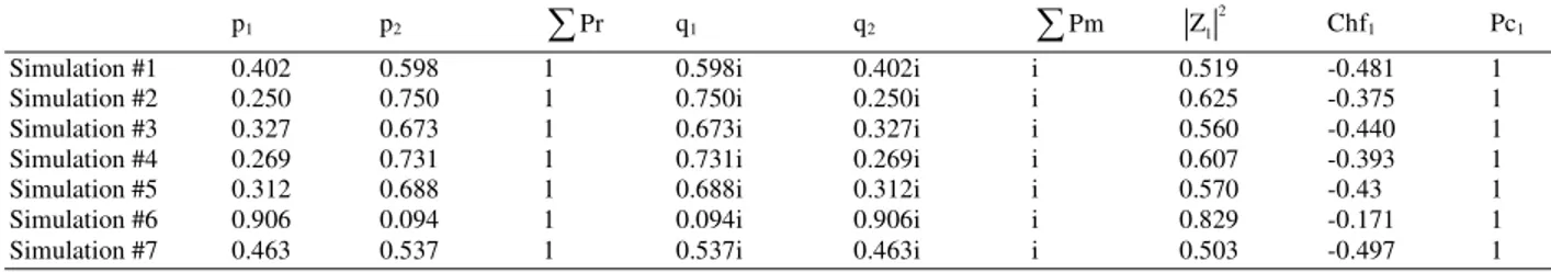
123 Table 1: Simulation of the Bernoulli distribution: Random draw of p1 (p2 = 1- p1)
p1 p2
∑
Pr q1 q2∑
Pm2 1
Z Chf1 Pc1
Simulation #1 0.402 0.598 1 0.598i 0.402i i 0.519 -0.481 1
Simulation #2 0.250 0.750 1 0.750i 0.250i i 0.625 -0.375 1
Simulation #3 0.327 0.673 1 0.673i 0.327i i 0.560 -0.440 1
Simulation #4 0.269 0.731 1 0.731i 0.269i i 0.607 -0.393 1
Simulation #5 0.312 0.688 1 0.688i 0.312i i 0.570 -0.43 1
Simulation #6 0.906 0.094 1 0.094i 0.906i i 0.829 -0.171 1
Simulation #7 0.463 0.537 1 0.537i 0.463i i 0.503 -0.497 1
Table 2: Simulation of the Binomial distribution: Consider N = 10 and k = 3
p1 q1 Prk Pmk
N k k 0
Pr
=
∑
N k k 0Pm
=
∑
2k
Z Chfk Pck
Simulation #1 0.608 0.392 0.038 0.962i 1 10i 0.9270 -0.073 1
Simulation #2 0.553 0.447 0.072 0.928i 1 10i 0.8660 -0.134 1
Simulation #3 0.012 0.988 0.0002 0.9998i 1 10i 0.9995 -0.0005 1
Simulation #4 0.319 0.681 0.265 0.735i 1 10i 0.6110 -0.389 1
Simulation #5 0.157 0.843 0.141 0.859i 1 10i 0.7580 -0.242 1
Simulation #6 0.442 0.558 0.175 0.825i 1 10i 0.7120 -0.288 1
Simulation #7 0.461 0.539 0.155 0.845i 1 10i 0.7370 -0.263 1
Fig. 4: Graph of the linear function Z2−Chf =1
In the simulations, the values of p1 are taken from the computer system by using the C++ predefined function rand( ) which is a pseudorandom number generator (Deitel and Deitel, 2003). The other values like p2,q1,q2 are deduced from p1. Hence, Monte Carlo simulation method proves numerically what has been found above theoretically (Cheney and Kincaid, 2004; Gentle James, 2003; Gerald and Wheatley, 2000; Liu, 2001; Muller, 2005; Robert and George, 2004).
CONCLUSION
The degree of our knowledge in the real universe R is unfortunately incomplete, hence the extension to the complex universe C that includes the contributions of both the real universe R and the imaginary universe M. Consequently, this will result in a complete and perfect degree of knowledge in C. This hypothesis is verified in this study by the mean of many examples encompassing both discrete and continuous domains. Moreover, we have proved a linear proportional relation between the degree of knowledge and the chaotic factor. In fact, in
order to have a certain prediction of any event it is necessary to work in the complex universe C in which the chaotic factor is quantified and subtracted from the degree of knowledge to lead to a probability in C equal to one. Thus, the study in the complex universe results in replacing the phenomena that used to be random in R by deterministic and totally predictable ones in C. In a future work, we will more develop the concept of complex probabilities and this by determining the characteristics (expectation, variance, and standard deviation) of what we called the complex random vectors. Moreover, we will prove using this key complex concept the very well known law of large numbers.
REFERENCES
Abou Jaoude Abdo, M., 2004. Numerical methods and algorithms for applied mathematicians. Ph.D. Thesis, Department of Applied Mathematics, Bircham International University.
Abou Jaoude Abdo, M., 2005. Computer simulation of monte carlo methods and random phenomena. Ph.D. Thesis, Department of Computer Science, Bircham International University.
Abou Jaoude Abdo, M., 2007. Analysis and algorithms for the statistical and stochastic paradigm. Ph.D. Thesis, Department of Applied Statistics and Probability, Bircham International University. Balibar, F., 1980. Albert Einstein: Physique,
Philosophie, Politique. 1st Edn., Paris, Le Seuil, ISBN: 2-02-039658-0, pp: 229-465.
124 Benton, W., 1966. Probability, Mathematical:
Encyclopedia Britannica. Encyclopedia Britannica Inc., Chicago, pp: 574-579.
Boursin, J.L., 1986. Structures of Ccance. Le Seuil, ISBN: 2-02-009235-2, pp : 5-33.
Chen, W., D. de Kee and P.N. Kaloni, 1997. Advanced Mathematics for Applied and Pure Sciences. Gordon and Breach Science Publishers, The Netherlands, ISBN: 90-5699-614-2, pp: 191-238. Cheney, E.W. and D.R. Kincaid, 2004. Numerical
Mathematics and Computing. 5th Edn., Thomson Brooks/Cole, ISBN: 0-534-8993-7, pp: 559-591. Dacunha-Castelle, D., 1996. Paths of Random. 1st Edn.,
Flammarion, ISBN: 2-08-081440-1, pp: 15-34. Dahan, D.A. and J. Peiffer, 1986. A History of
Mathhematics. 1st Edn., Edition du Seuil, ISBN: 2-02009138-0, pp: 248-262.
Dahan, D.A., J.L. Chabert and K. Chemla, 1992. Chaos and Determinism. 1st Edn., Edition du Seuil, ISBN: 2-02-015182-0, pp: 11-90.
Ducrocq, A. and A. Warusfel, 2004. Mathematics, pleasure and necessity. 1st Edn., Vuibert, ISBN: 2-02-061261-5, pp: 45-77.
Deitel, H.M. and P.J. Deitel, 2003. C++ How to Program. 4th Edn., Prentice Hall, ISBN: 0-13-111881-1, pp: 183-190.
Ekeland, I., 1991. Random. Luck, Science and the World. 1st Edn., Editions du Seuil, ISBN: 2-02-0012877-2, pp: 11-99.
Gentle James, E., 2003. Random Number Generation and Monte Carlo Methods. 2nd Edn., Springer, ISBN: 0-387-00178-6, pp: 229-261.
Gerald, C.F. and P.O. Wheatley, 2000. Applied Numerical Analysis. 5th Edn., Addison Wesley, ISBN: 0-201-59290-8, pp: 42.
Gleick, J., 1997. Chaos, Making a New Science. 1st Edn., Penguin Books, ISBN: 10: 0140092501, pp: 213-240.
Greene, B., 2000. The Elegant Universe. 1st Edn., Vintage Books, New York, ISBN: 0-375-70811-1, pp: 135-210.
Greene, B., 2004. The Fabric of the Cosmos. 1st Edn., Vintage Books, New York, ISBN: 0-375-72720-5, pp: 143-176.
Hoffmann, B., H. Dukas and A. Einstein, 1975. Creator and Rebel. 1st Edn., Editions du Seuil, ISBN: 2-02-002120-X, pp: 229-239.
Khaled, E.T., 2002. Random mechanics and maintenance. Lecture course for Master2R Mechanics, Lebanese University, Graduate School of Science and Technology, Beirut, Lebanon.
Kuhn, T., 1970. The Structure of Scientific Revolutions. 2nd Edn., Chicago Press, Chicago, pp: 7-33.
Liu, J.S., 2001. Monte Carlo Strategies in Scientific Computing. 1st Edn., Springer, ISBN: 0-387-95230-6, pp: 53-77.
Montgomery, C.D. and R.C. George, 2003. Applied Statistics and Probability for Engineers. 3rd Edn., John Wiley and Sons, Inc., ISBN: 0-471-20454-4, pp : 16-53.
Muller, X., 2005. Mathematics: The computer will soon have the last word. Science, 1056: 33-40.
Orluc, L. and P. Herve, 2005. Generating fractal mandelbrot children. Science, 1056: 41-47.
Poincare, H., 1968. Science and hypothese. 1st Edn., Flammarion, Paris, ISBN: 2-08-081056-1, pp: 191-214.
Prigogine, I. and S. Isabelle, 1992. Between Time and Entry. 1st Edn., Flammarion, Paris, ISBN: 01-02-85080, pp: 69-93.
Prigogine, I., 1997. The End of Certainty. 1st Edn., The Free Press, ISBN: 0-684-83705-6, pp: 73-89. Robert, C. and C. George, 2004. Monte Carlo Statistical
Methods. 2nd Edn., Springer, ISBN: 0-387-21239-6, pp: 35-57.
Srinivasan, S.K. and K.M. Mehata, 1988. Stochastic Processes. 2nd Edn., McGraw-Hill, New Delhi, ISBN: 0-07-451938-7, pp: 1-45.
Stewart, I., 1996. From Here to Infinity. 2nd Edn., Oxford University Press, ISBN: 0-19-283202-6, pp: 216-237.
Stewart, I., 2002. Does God Play Dice? 2nd Edn., Blackwell Publishing, ISBN: 0-631-23251-6, pp: 1-18.
Van Kampen, N.G., 2006. Stochastic Processes in Physics and Chemistry. Elsevier, The Netherlands, ISBN: 0-444-89349-0, pp: 1-70.
Walpole, R.E., R.H. Myers and S.L. Myers, 2002. Probability and Statistics for Engineers and Scientists. 7th Edn., Prentice Hall, ISBN: 0-13-098469-8, pp: 22-61.