© 2014 Science Publications
doi:10.3844/jmssp.2014.1.24 Published Online 10 (1) 2014 (http://www.thescipub.com/jmss.toc)
COMPLEX PROBABILITY THEORY AND PROGNOSTIC
Abdo Abou Jaoude
Department of Mathematics and Statistics,
Faculty of Natural and Applied Sciences, Notre Dame University, Zouk Mosbeh, Lebanon
Received 2013-08-27; Revised 2013-10-06; Accepted 2013-10-09
ABSTRACT
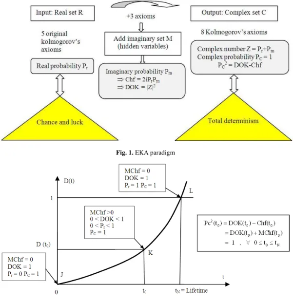
The Kolmogorov’s system of axioms can be extended to encompass the imaginary set of numbers and this by adding to the original five axioms an additional three axioms. Hence, any experiment can thus be executed in what is now the complex set C (Real set R with real probability + Imaginary set M with imaginary probability). The objective here is to evaluate the complex probabilities by considering supplementary new imaginary dimensions to the event occurring in the “real” laboratory. Whatever the probability distribution of the input random variable in R is, the corresponding probability in the whole set C is always one, so the outcome of the random experiment in C can be predicted totally. The result indicates that chance and luck in R is replaced now by total determinism in C. This new complex probability model will be applied to the concepts of degradation and the Remaining Useful Lifetime (RUL), thus to the field of prognostic.
Keywords: Complex Probability, Probability Distributions, Prognostic, Degradation, Lifetime
1. INTRODUCTION
Abou Jaoude et al. (2010); Abou Jaoude (2013; 2005; 2007); Bell (1992); Benton (1996); Boursin (1986); Chen et al. (1997); Cheney and Kincaid (2004); Dacunha-Castelle (1999); Dalmédico Dahan et al. (1992); Dalmedico Dahan and Peiffer (1986); Ekeland (1991); Feller (1968); Finney et al. (2004); Gentle (2003); Gerald and Wheatley (1999); Gleick (1997); Greene (2000; 2004) firstly, the Extended Kolmogorov’s Axioms (EKA for short) paradigm can be illustrated by the following figure (Fig. 1).
In engineering systems, the remaining useful lifetime prediction is related deeply to many factors that generally have a chaotic behavior which decreases the degree of our knowledge of the system.
As the Degree of Our Knowledge (DOK for short) in the real universe R is unfortunately incomplete, the extension to the complex universe C includes the contributions of both the real universe R and the imaginary universe M. Consequently, this will result in a complete and perfect degree of knowledge in C = R+M (Pc = 1). In fact, in order to have a certain prediction of any event it is necessary to work in the complex universe C in which the chaotic factor is quantified and subtracted from the Degree Of Knowledge to lead to a probability
in C equal to one (Pc2 = DOK-Chf = 1). Thus, the study in the complex universe results in replacing the phenomena that used to be random in R by deterministic and totally predictable ones in C.
This hypothesis is verified in a previous study and paper by the mean of many examples encompassing both discrete and continuous distributions.
From the Extended Kolmogorov’s Axioms (EKA), we can deduce that if we add to an event probability in the real set R the imaginary part M (like the lifetime variables) then we can predict the exact probability of the remaining lifetime with certainty in C (Pc = 1).
We can apply this idea to prognostic analysis through the degradation evolution of a system. As a matter of fact, prognostic analysis consists in the prediction of the remaining useful lifetime of a system at any instant t0 and during the system functioning.
Let us consider a degradation trajectory D(t) of a system where a specific instant t0 is studied. The instant t0 means here the time or age that can be measured also by the cycle number N.
Fig. 1. EKA paradigm
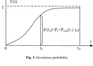
Fig. 2. EKA and the prognostic of degradation
In fact, at the beginning (t0 = 0) (point J), the failure probability Pr = 0 and the chaotic factor in our prediction is zero (Chf = 0). Therefore, RUL(t0 = 0) = tN-t0 = tN.
If t0 = tN (point L) then the RUL(tN) = tN-tN = 0 and the failure probability is one (Pr = 1).
If not (i.e., 0<t0<tN) (point K), the probability of the occurrence of this instant and the prediction probability of RUL are both less than one (not certain) due to non-zero chaotic factors. The degree of our knowledge is consequently less than 1. Thus, by applying here the EKA method, we can determine the system RUL with certainty in C = R+M where Pc = 1 always.
Furthermore, we need in our current study the absolute value of the chaotic factor that will give us the magnitude of the chaotic and random effects on the studied system. This new term will be denoted accordingly MChf or Magnitude of the Chaotic Factor. Hence, we can deduce the following:
0 0
2
0 0 0 0 0
0
0 0 0 N
0 0
MChf(t ) Chf(t ) 0 and
Pc (t ) DOK(t ) Chf(t ) DOK(t ) Chf(t ) , since 0.5 Chf(t ) 0
DOK(t ) MChf(t ) 1, 0 t t 0 MChf(t ) 0.5 where 0.5 DOK(t ) 1
= ≥
= − = +
− ≤ ≤
= + = ∀ ≤ ≤
Moreover, we can define two complementary events E and Ewith their respective probabilities:
rob rob
P (E)=p and P (E)= = −q 1 p
Then Prob (E) in terms of the instant t0 is given by: Prob (E) = Pr = Prob (t≤t0) = F(t0) where F is the cumulative probability distribution function of the random variable t.
Since Prob (E)+Prob(Ē)= 1, therefore, Prob(Ē) = 1-Prob(E) = 1-Pr = 1-Prob(t≤t0)= Prob (t>t0).
Let us define the two particular instants: t0 = 0 assumed as the initial time of functioning (raw state) corresponding to D = D0 = 0 and tN = the failure instant (wear out state) corresponding to the degradation D = 1.
The boundary conditions are.
For t0 = 0 then D = D0 (initial damage that may be zero or not) and F (t0) = Prob (t≤0) = 0.
For t0 = tN then D = 1 and F(t0) = F (tN) = Prob (t≤tN) = 1. Also F(t0) is a non-decreasing function that varies between 0 and 1. In fact, F(t0) is a cumulative function (Fig. 3). In addition, since RUL(t0) = tN-t0 and 0≤t0≤tN then RUL(t0) is a non-increasing remaining useful lifetime function (Fig. 4).
Referring to Fig. 5 below, we can infer the following: The complex probability Z(t0) = Pr(t0)+Pm(t0) = Pr(t0)+i[1-Pr(t0)].
The square of the norm of Z(t0) is:
( )
( ) ( )
( )
( )
( )
( )
2
0 0 r 0 m 0
2
r 0 r 0 r 0 r 0
Z(t ) DOK t 1 2iP t P t
1 2P t 1 P t 1 2P t 2P t
= = +
= − − = − +
The Chaotic Factor and the Magnitude of the Chaotic Factor are:
Chf(t0) = -2Pr(t0)[1-Pr(t0)] = -2Pr(t0)+2Pr2(t0) is null when Pr(t0) = Pr(0) = 0 (point J) or when Pr(t0) = Pr(tN) = 1 (point L) and MChf(t0) = |Chf(t0)| = 2Pr(t0)[1-Pr(t0)] = 2Pr(t0)-2Pr2(t0) is null when Pr(t0) = Pr(0) = 0 (point J) or when Pr(t0) = Pr(tN) = 1 (point L)
At any instant t0 (point K), the probability expressed in the complex set C is:
Pc(t0) = Pr(t0)+Pm(t0)/i = Pr(t0)+[1-Pr(t0)] = 1 always. Hence, the prediction of RUL(t0) of the system degradation in C is permanently certain.
Let us consider thereafter many probability distributions to model the function F(t0).
2. APPLICATION TO DIFFERENT
PROBABILITY DISTRIBUTIONS
2.1. The
Uniform Probability
Distribution
(Guillen, 1995; Gullberg, 1997; Kuhn,
1996;
Liu,
2001;
Mandelbrot,
1997;
Montgomery and Runger, 2005; M
ũ
ller,
2005; Orluc and Poirier, 2005; Poincaré,
1968; Prigogine, 1997; Prigogine and
Stengers, 1992; Robert and Casella, 2010;
Science et Vie, 1999; Srinivasan and Mehata,
1978; Stewart, 1996; 2002; Van Kampen,
2007; Walpole, 2002; Ducrocq and Warusfel,
2004; Weinberg, 1992)
With a probability density function:
1
if a t b dF(t)
f(t) b a
dt
0 elsewhere
≤ ≤
= = −
and a cumulative distribution function:
(
)
t0 t0 00 0 rob 0
a
t a
if a t b F(t ) P t t f(t)dt f(t)dt b a
0 elsewhere
−∞
−
≤ ≤
= ≤ = = = −
∫
∫
With the two boundaries a = 0 and b = tN then:
0 0
0 0 N
N N
t 0 t
F(t ) if 0 t t
t 0 t
−
= = ≤ ≤
−
We have taken the domain for the uniform variable t0= [0, tN = 1000] and dt0 = 0.1 then:
0
0 0
t
F(t ) if 0 t 1000 1000
= ≤ ≤
2.1.1. The Real Probability P
r:
0
r 0 0 0 N
N
t
P (t ) F(t ) if 0 t t 1000 t
= = ≤ ≤ =
We note that Pr(t0) is a non-decreasing function.
2.1.2. The Complementary Probability P
m/i:
0
m 0 r 0 0 0 N
N
t
P (t ) / i 1 P (t ) 1 F(t ) 1 if 0 t t 1000 t
Fig. 4. RUL prognostic model
We note that Pm (t0)/i is a non-increasing function.
2.1.3. The Degree of Our Knowledge DOK
DOK is the measure of our certain knowledge (100% probability) about the expected event, it does not include any uncertain knowledge (with probability less than 100%):
[
]
[
]
2
0 0 r 0 m 0
rob rob r 0 r 0
0 0 0 0 N N 2 0 0 N N
DOK(t ) Pc (t ) 2iP (t )P (t )
1 2.P (E).P (E) 1 2.P (t ). 1 P (t )
t t
1 2.F(t ). 1 F(t ) 1 2. . 1
t t
t t
1 2. 2.
t t = + = − = − − = − − = − − = − +
Which is a parabola concave upward having a vertex (a minimum) at:
3 N
0
t
t 500 0.5 10 , 0.5 2
= = = ×
2.1.4. The Chaotic Factor Chf and MChf:
[
]
[
]
0 r 0 m 0 rob rob
r 0 r 0 0 0
2
0 0 0 0
N N N N
Chf (t ) 2iP (t )P (t ) 2.P (E).P (E)
2.P (t ). 1 P (t ) 2.F(t ). 1 F(t )
t t t t
2. . 1 2. 2.
t t t t
= = −
= − − = − −
= − − = − +
Which is a parabola concave upward having a vertex (a minimum) at:
3 N
0
t
t 500 0.5 10 , 0.5 2
= = = × −
Therefore, we can infer the magnitude of the chaotic factor MChf:
[
]
[
]
[
]
0 0 r 0 r 0
r 0 r 0 0 0
2
0 0 0 0
N N N N
MChf (t ) Chf (t ) 2.P (t ). 1 P (t )
2.P (t ). 1 P (t ) 2.F(t ). 1 F(t )
t t t t
2. . 1 2. 2.
t t t t
= = − −
= − = −
= − = −
Which is a parabola concave downward having a vertex (a maximum) at:
3 N
0
t
t 500 0.5 10 , 0.5 2
= = = ×
2.1.5. Pc: The Probability in the Complex Set C:
2
0 0 0
2 2
0 0 0 0
0
N N N N
Pc (t ) DOK(t ) Chf(t )
t t t t
1 2. 2. 2. 2. 1 Pc(t ) 1
t t t t
= −
= − + + − = ⇒ =
Thus we deduce that in the set C, we have a complete knowledge of the random variable since Pc = 1.
2.1.6. The Intersection Point:
0 0 0
r 0 m 0
N N N
N 0
r 0
m 0
t t t
P (t ) P (t ) / i 1 2.
t t t
t 1000
1 t 500
2 2
500
and P (t 500) 0.5 and 1000
500
P (t 500) / i 1 1 0.5 0.5 1000
= ⇔ = − ⇔
= ⇔ = = =
= = =
= = − = − =
So Pr(t0) and Pm(t0)/i intersect at (500, 0.5).
Moreover, the minimum of DOK and the maximum of MChf occur at (500, 0.5).
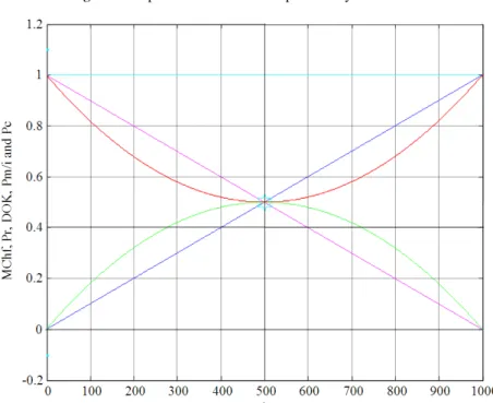
So we conclude that Pr(t0), Pm(t0)/i, DOK and MChf all intersect at (500, 0.5) (Fig. 6-9).
2.1.7. The EKA Parameters Analysis in the
Prognostic of Degradation:
We note from the figure below that the DOK is maximum (DOK = 1) when MChf is minimum (MChf = 0) (points J & L) and that means when the magnitude of the chaotic factor (MChf) decreases our certain knowledge increases.
At the beginning Pr (t0)= t0/tN = 0/tN = 0, the system is intact (zero damage: D = 0) and has zero chaotic factor before any usage, at this instant DOK(0) = 1 and RUL(0) = tN-0 = tN with Pc(0) = 1. Afterward, 0<t0<tN, RUL(t0) = tN-t0 with Pr(t0) = t0/tN ≠ 0 and Pc(t0) = 1 and MChf starts to increase during the functioning due to the environment and intrinsic conditions thus leading to a decrease in DOK until they both reach 0.5 at t0 = tN/2 = 500 (point K) where RUL(tN/2) = tN/2 = 500. Since the real probability Pr is a uniform distribution MChf will intersect with DOK at the point (tN/2 = 500, 0.5) (point K).
Fig. 6. EKA parameters in uniform probability distribution
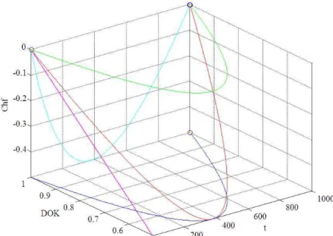
Fig. 8.The probabilities Pr and Pm / i in terms of t and of each other
Fig. 10. EKA parameters and the prognostic of degradation
We note that the same logic and analysis apply concerning the degradation and the remaining useful lifetime for the all the six probability distributions.
2.2. The Logarithmic Distribution:
With a probability density function:
N
α
if 0 t t dF(t)
f(t) 1 αt dt
0 elsewhere where α (e 1) / 1000 0.001718281...
≤ ≤
= = +
= − =
and a cumulative distribution function:
0 0
t t
0 0 N
0
0
Ln(1 t ) if 0 t t F(t ) f(t)dt f(t)dt
0 elsewhere
−∞
+ α ≤ ≤
= = =
∫
∫
We have taken the domain for the logarithmic variable t0= [0, tN = 1000] where dt0 = 0.1.
2.2.1. The Real Probability P
r:
r 0 0 0 N
P =F(t )=Ln(1+ αt ) if 0≤ ≤t t =1000
We note that Pr is a non-decreasing function.
2.2.2. The Complementary Probability P
m/i:
m r 0 0
0 N
P / i 1 P 1 F(t ) 1 Ln(1 t ) if 0 t t 1000
= − = − = − + α
≤ ≤ =
We note that Pm/i is a non-increasing function.
2.2.3. The Degree of Our Knowledge DOK:
DOK is the measure of our certain knowledge (100% probability) about the expected event, it does not include any uncertain knowledge (with probability less than 100%):
[
]
[
]
[
]
r r rob rob
0 0
0 0
2
0 0
DOK 1 2.P .(1 P ) 1 2.P (E).P (E)
1 2.F(t ). 1 F(t )
1 2.Ln(1 t ). 1 Ln(1 t )
1 2.Ln(1 t ) 2 Ln(1 t )
= − − = −
= − −
= − + α − + α
= − + α + + α
which is a curve concave upward having a minimum at:
(
t0=377.54, 0.5)
2.2.4. The Chaotic Factor Chf and MChf:
(
)
[
]
[
]
[
]
r r rob rob
0 0
0 0
2
0 0
Chf 2.P . 1 P 2.P (E).P (E)
2.F(t ). 1 F(t )
2.Ln(1 t ). 1 Ln(1 t )
2.Ln(1 t ) 2. Ln(1 t )
= − − = −
= − −
= − + α − + α
= − + α + + α
which is a curve concave upward having a minimum at:
Therefore, we can infer the magnitude of the chaotic factor MChf:
[
]
[
]
[
]
[
]
[
]
0 0 r 0 r 0
r 0 r 0 0 0
0 0
2
0 0
MChf (t ) Chf (t ) 2.P (t ). 1 P (t )
2.P (t ). 1 P (t ) 2.F(t ). 1 F(t )
2.Ln(1 t ). 1 Ln(1 t )
2.Ln(1 t ) 2. Ln(1 t )
= = − −
= − = −
= + α − + α
= + α − + α
Which is a curve concave downward having a maximum at:
(
t0=377.54, 0.5)
2.2.5. Pc: The Probability in the Complex Set C:
[
]
[
]
2 2 0 0 2 0 0Pc DOK Chf 1 2.ln(1 t ) 2. ln(1 t )
2.ln(1 t ) 2. ln(1 t ) 1 Pc 1
= − = − + α + + α
+ + α − + α = ⇒ =
Thus we deduce that in the set C, we have a complete knowledge of the random variable since Pc = 1.
2.2.6. The Intersection Point:
(
)
r 0 m 0 0 0
0 0
0
r 0
m 0
P (t ) P (t ) / i Ln(1 t ) 1 Ln(1 t ) 1
2.Ln(1 t ) 1 Ln(1 t ) 2 t exp(0.5) 1 / 377.54
and P (t 377.54) Ln(1 377.54) 0.5 and P (t 377.54) / i 1 Ln(1 377.54)
1 0.5 0.5
= ⇔ + α = − + α
⇔ + α = ⇔ + α =
⇔ = − α =
= = + α × =
= = − + α ×
= − =
So Pr(t0) and Pm(t0)/i intersect at (377.54, 0.5). Moreover, the minimum of DOK and the maximum of MChf occur at (377.54, 0.5).
So we conclude that Pr(t0), Pm(t0)/i, DOK and MChf all intersect at (377.54, 0.5) (Fig. 11-13).
2.2.7. The EKA Parameters Analysis in the
Prognostic of Degradation:
In this case, we note from the figure below that the DOK is maximum (DOK = 1) when MChf is minimum (MChf = 0) (points J & L). Afterward, MChf starts to increase with the decrease of DOK until it reaches 0.5 at t0 = 377.54 (point K). Since the
real probability Pr is a logarithmic distribution (convex curve) it will intersect with DOK at the point (377.54, 0.5) (point K). With the increase of t0, MChf returns to zero and the DOK returns to 1 where we reach total damage (D = 1) and hence the total certain failure (Pr = 1) of the system (point L). We note that the point K is no more at the middle of DOK since the distribution is not anymore uniform and symmetric.
At each instant t0, the remaining useful lifetime RUL(t0) is certainly predicted in the complex set C with Pc maintained as equal to one through a continuous compensation between DOK and Chf. This compensation is from instant t0 = 0 where D(t0) = 0 until the failure instant tN where D(tN) = 1 (Fig. 11).
2.3. The Power Probability Distribution:
With a probability density function:
13
N 14
14.t
dF(t) if 0 t t
f(t) 1000 dt 0 elsewhere ≤ ≤ = =
and a cumulative distribution function:
0 0
14
t t 0
0 N 14
0
0
t
if 0 t t F(t ) f(t)dt f(t)dt 1000
0 elsewhere −∞ ≤ ≤ = = =
∫
∫
We have taken the domain for the power variable t0 = [0,tN = 1000] and dt0 = 0.1.
2.3.1. The Real Probability P
r:
14 0
r 0 14 0 N
t
P F(t ) if 0 t t 1000 1000
= = ≤ ≤ =
We note that Pr is a non-decreasing function.
2.3.2. The Complementary Probability P
m/i:
14 0
m r 0 14
0 N
t P / i 1 P 1 F(t ) 1
1000 if 0 t t 1000
= − = − = −
≤ ≤ =
Fig. 11.EKA parameters in logarithmic cumulative distribution
Fig. 13.DOK and Chf in terms of t and of each other in logarithmic cumulative distribution
2.3.3. The Degree of Our Knowledge DOK:
DOK is the measure of our certain knowledge (100% probability) about the expected event, it does not include any uncertain knowledge (with probability less than 100 %):
[
r r]
rob rob0 0
14 14 14
0 0 0
14 14 14
2
14 14 28
0 0 0
14 14 28
DOK 1 2.P .(1 P ) 1 2.P (E).P (E) 1 2.F(t ). 1 F(t )
t t t
1 2. . 1 1 2.
1000 1000 1000
t t t
2. 1 2. 2.
1000 1000 1000
= − − = −
= − −
= − − = −
+ = − +
Which is a curve concave upward having a minimum at:
(
t0=951.7, 0.5)
2.3.4. The Chaotic Factor Chf and MChf:
(
)
[
]
r r rob rob
0 0
2
14 14 14 14
0 0 0 0
14 14 14 14
14 28
0 0
14 28
Chf 2.P . 1 P 2.P (E).P (E)
2.F(t ). 1 F(t )
t t t t
2. . 1 2. 2.
1000 1000 1000 1000
t t
2. 2.
1000 1000
= − − = −
= − −
= − − = − +
= − +
Which is a curve concave upward having a minimum at:
(
t0=951.7, −0.5)
Therefore, we can infer the magnitude of the chaotic factor MChf:
[
]
[
]
[
]
0 0 r 0 r 0
r 0 r 0 0 0
14 14 14 28
0 0 0 0
14 14 14 28
MChf (t ) Chf (t ) 2.P (t ). 1 P (t )
2.P (t ). 1 P (t ) 2.F(t ). 1 F(t )
t t t t
2. . 1 2. 2.
1000 1000 1000 1000
= = − −
= − = −
= − = −
Which is a curve concave downward having a maximum at:
(
t0=951.7, 0.5)
2.3.5. Pc: The Probability in the Complex Set C:
2
14 14
2 0 0
14 14
2
14 14
0 0
14 14
t t
Pc DOK Chf 1 2. 2. 1000 1000
t t
2. 2. 1 Pc 1
1000 1000
= − = − +
+ − = ⇒ =
So Pr(t0) and Pm(t0)/i intersect at (951.7, 0.5).
Moreover, the minimum of DOK and the maximum of MChf occur at (951.7, 0.5).
So we conclude that Pr(t0), Pm(t0)/i, DOK and MChf all intersect at (951.7, 0.5) (Fig. 14-16).
2.3.7. The EKA Parameters Analysis in the
Prognostic of Degradation:
In this case, we note from the figure below that the DOK is maximum (DOK=1) when MChf is minimum (MChf = 0) (points J & L). Afterward, MChf starts to increase with the decrease of DOK until it reaches 0.5 at t0 = 951.7 (point K). Since the real probability Pr is a power distribution it will intersect with DOK at the point (951.7, 0.5) (point K). With the increase of t0, MChf returns to zero and the DOK returns to 1 where we reach total damage (D =1) and hence the total certain failure (Pr = 1) of the system (point L). At this last point L the failure here is certain, Pr(tN) = tN/tN = 1 and RUL(tN) = tN-tN = 0 with Pc(tN) = 1, so the logical explanation of the value DOK = 1 follows. We note that the point K is no more at the middle of DOK since the distribution is neither uniform nor symmetric (Fig. 14).
2.4. The Exponential Probability Distribution:
With a probability density function:
(
)
N
1000 t 1
exp if 0 t t
dF(t)
f(t) 200 200
dt
0 elsewhere
−
− ≤ ≤
= =
and a cumulative distribution function:
0 N
if 0≤ ≤t t =1000
We note that Pr is a non-decreasing function.
2.4.2. The Complementary Probability P
m/i:
(
0)
m r 0
0 N
1000 t P / i 1 P 1 F(t ) 1 exp
200 if 0 t t 1000
−
= − = − = − −
≤ ≤ =
We note that Pm/i is a non-increasing function.
2.4.3. The Degree of Our Knowledge DOK:
DOK is the measure of our certain knowledge (100% probability) about the expected event, it does not include any uncertain knowledge (with probability less than 100%):
[
]
(
)
(
)
(
)
(
)
(
)
r r rob rob
0 0
0 0
2
0 0
0
DOK 1 2.P .(1 P ) 1 2.P (E).P (E) 1 2.F(t ). 1 F(t )
1000 t 1000 t
1 2.exp . 1 exp
200 200
1000 t 1000 t
1 2.exp 2. exp
200 200
1000 t
1 2.exp 2.exp
200
= − − = −
= − −
− −
= − − − −
− −
= − − + −
−
= − − + −
(
0)
2. 1000 t 200
−
Which is a curve concave upward having a minimum at:
Fig. 14.EKA parameters in power probability distribution
Fig. 16.DOK and Chf in terms of t and of each other in power probability distribution
2.4.4. The Chaotic Factor Chf and MChf:
(
)
[
]
(
)
(
)
(
)
(
)
(
)
r r rob rob
0 0
0 0
2
0 0
0
Chf 2.P . 1 P 2.P (E).P (E)
2.F(t ). 1 F(t )
1000 t 1000 t
2.exp . 1 exp
200 200
1000 t 1000 t
2.exp 2. exp
200 200 1000 t 2.exp = − − = − = − − − − = − − − − − − = − − + − −
= − − 2. 1000
(
t0)
2.exp 200 200 − + −
Which is a curve concave upward having a minimum at:
(
t0=861.37, −0.5)
Therefore, we can infer the magnitude of the chaotic factor MChf:
[
]
[
]
[
]
(
)
(
)
(
)
(
)
0 0 r 0 r 0
r 0 r 0 0 0
0 0
0 0
MChf (t ) Chf (t ) 2.P (t ). 1 P (t )
2.P (t ). 1 P (t ) 2.F(t ). 1 F(t )
1000 t 1000 t
2.exp . 1 exp
200 200
1000 t 2. 1000 t 2.exp 2.exp 200 200 = = − − = − = − − − = − − − − − = − − −
Which is a curve concave downward having a maximum at:
(
t0=861.37, 0.5)
2.4.5. Pc: The Probability in the Complex Set C:
(
)
(
)
(
)
(
)
0 2 2 0 2 0 0 1000 tPc DOK Chf 1 2.exp
200
1000 t 2. exp
200
1000 t 1000 t
2.exp 2. exp 1
200 200 Pc 1 − = − = − − − + − − − + − − − = ⇒ =
Thus we deduce that in the set C, we have a complete knowledge of the random variable since Pc = 1.
2.4.6. The Intersection Point:
(
)
(
)
(
)
(
)
(
)
0 r 0 m 0
0 0 0 0 r 0 m 0 1000 t P (t ) P (t ) / i exp
200
1000 t 1000 t
1 exp 2.exp 1
200 200
1000 t 1 exp
200 2
t 1000 200.Ln(0.5) 861.37
1000 861.37
And P (t 861.37) exp 0.5
200
and P (t 861.37) / i 1
− = ⇔ − − − = − − ⇔ − = − ⇔ − = ⇔ = + = − = = − =
= = exp
(
1000 861.37)
200 1 0.5 0.5 −
− −
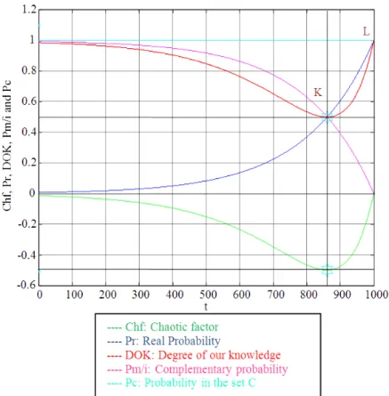
Fig. 17. EKA parameters in exponential cumulative distribution
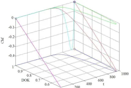
Fig. 19. DOK and Chf in terms of t and of each other in exponential cumulative distribution
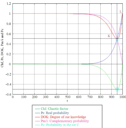
So Pr(t0) and Pm(t0)/i intersect at (861.37, 0.5). Moreover, the minimum of DOK and the maximum of MChf occur at (861.37, 0.5).
So we conclude that Pr(t0), Pm(t0)/i, DOK and MChf all intersect at (861.37, 0.5) (Fig. 17-19).
2.4.7. The EKA Parameters Analysis in the
Prognostic of Degradation:
In this case, we note from the figure above that the DOK is maximum (DOK=1) when MChf is minimum (MChf=0) (points J & L). Afterward, the magnitude of the chaotic factor MChf starts to increase with the decrease of DOK until it reaches 0.5 at t0=861.37 (point K). Since the real probability Pr is an exponential distribution it will intersect with DOK at the point (861.37, 0.5) (point K). With the increase of t0, Chf and MChf return to zero and the DOK returns to 1 where we reach total damage (D = 1) and hence the total certain failure (Pr = 1) of the system (point L). At this last point L the failure here is certain, Pr(tN) = tN/tN = 1 and RUL(tN) = tN-tN = 0 with Pc(tN) = 1, so the logical explanation of the value DOK = 1 follows. We note that the point K is no more at the middle of DOK since the exponential distribution is not symmetric (Fig. 17).
2.5. The Normal Probability Distribution:
With a probability density function:
2
t t
dF(t) 1 1 t t
f(t) exp ,
dt 2πσ 2 σ
for t
−
= = −
− ∞ < < ∞
and a cumulative distribution function:
0 0 0 2
t t t
0
t
0 0 t
0 N
1 1 t t
F(t ) f(t)dt f(t)dt exp .dt, 2 σ
2πσ
for 0 t t
−∞
−
= = = −
≤ ≤
∫
∫
∫
We have taken the domain for the normal variable t0 = [0, tN = 1000], dt0 = 0.1, t=500 (Mean) and σt = 150 (Standard deviation).
Note that:
2
t t
1 1 t t
dF f(t)dt exp .dt 1
2 σ
2πσ
+∞ +∞ +∞
−∞ −∞ −∞
−
= = − =
∫
∫
∫
2.5.1. The Real Probability P
r:
0 2
t
r 0 0
t
0 t
0 N
1 1 t t
P (t ) F(t ) exp .dt
2 σ
2πσ
if 0 t t 1000
−
= = −
≤ ≤ =
∫
2.5.2. The Complementary Probability P
m/i:
0
N
0
m 0 r 0 0
2 t t 0 t 2 t t t t 0 N
P (t ) / i 1 P (t ) 1 F(t )
1 1 t t
1 exp .dt
2 σ
2πσ
1 1 t t
exp .dt
2 σ
2πσ
if 0 t t 1000
= − = − − = − − − = − ≤ ≤ =
∫
∫
We note that Pm(t0)/i is a non-increasing function.
2.5.3. The Degree of Our Knowledge DOK:
DOK is the measure of our certain knowledge (100% probability) about the expected event, it does not include any uncertain knowledge (with probability less than 100%).
[
]
[
]
0N
0
2
0 0 r 0 m 0
rob rob r 0 r 0
2 t 0 0 t 0 t 2 t t t t 2 t t
DOK(t ) Pc (t ) 2iP (t )P (t )
1 2.P (E).P (E) 1 2.P (t ). 1 P (t )
1 1 t t
1 2.F(t ). 1 F(t ) 1 2. exp .dt 2 σ
2πσ
1 1 t t
exp .dt
2 σ
2πσ
1 1 t t
1 2. exp
2 σ 2πσ = + = − = − − − = − − = − − − × − − = − −
∫
∫
0 0 t 0 2 2 t t 0 t .dt1 1 t t
2. exp .dt
2 σ 2πσ − + −
∫
∫
Which is a curve concave upward having a minimum at:
(
)
0 2 t t 0 t 01 1 t t
exp .dt
2 σ
2πσ
0.5 At t t 500, 0.5
− − = ⇔ = =
∫
Since the normal distribution is symmetric about the mean which is t=500.
2.5.4. The Chaotic Factor Chf and MChf:
[
]
[
]
0 r 0 m 0 rob rob
r 0 r 0 0 0
Chf (t ) 2iP (t )P (t ) 2.P (E).P (E)
2.P (t ). 1 P (t ) 2.F(t ). 1 F(t )
= = − = − − = − − 0 N 0 0 0 2 t t 0 t 2 t t t t 2 t t 0 t 2 2 t t 0 t
1 1 t t
2. exp .dt
2 σ
2πσ
1 1 t t
exp .dt
2 σ
2πσ
1 1 t t
2. exp .dt
2 σ
2πσ
1 1 t t
2. exp .dt
2 σ 2πσ − = − − − × − − = − − − + −
∫
∫
∫
∫
Which is a curve concave upward having a minimum at:
(
)
0 2 t t 0 t 01 1 t t
exp .dt
2 σ
2πσ
0.5 At t t 500, 0.5
− − = ⇔ = = −
∫
Since the normal distribution is symmetric about the mean which is t=500.
Therefore, we can infer the magnitude of the chaotic factor MChf:
[
]
[
]
[
]
0 N 0 00 0 r 0 r 0
r 0 r 0 0 0
2 t t 0 t 2 t t t t 2 t t 0 t t
MChf (t ) Chf (t ) 2.P (t ). 1 P (t )
2.P (t ). 1 P (t ) 2.F(t ). 1 F(t )
1 1 t t
2. exp .dt
2 σ
2πσ
1 1 t t
exp .dt
2 σ
2πσ
1 1 t t
2. exp .dt
2 σ 2πσ 1 2. e 2πσ = = − − = − = − − = − − × − − = − −
∫
∫
∫
0 2 2 t t 01 t t
xp .dt 2 σ − −
∫
Which is a curve concave downward having a maximum at:
(
)
0 2 t t 0 t 01 1 t t
exp .dt
2 σ
2πσ
0.5 At t t 500, 0.5
− − = ⇔ = =
∫
0 t
t t
0
2 2
Pc(t ) 1
⇒ =
Thus we deduce that in the set C, we have a complete knowledge of the random variable since Pc = 1.
2.5.6. The Intersection Point:
0 0 0 0 2 t
r 0 m 0
t 0 t 2 t t 0 t 2 t t 0 t 2 t t 0 t 0 r
1 1 t t
P (t ) P (t ) / i exp .dt 2 σ
2πσ
1 1 t t
1 exp .dt
2 σ
2πσ
1 1 t t
2. exp .dt 1
2 σ
2πσ
1 1 t t 1
exp .dt, 0.5
2 σ 2
2πσ
t t 500 and P
− = ⇔ − − = − − − ⇔ − = − ⇔ − = = ⇔ = =
∫
∫
∫
∫
0 m 0(t t 500) 0.5
and P (t t 500) / i 1 0.5 0.5
= = =
= = = − =
So Pr(t0) and Pm(t0)/i intersect at (500, 0.5).
Moreover, the minimum of DOK and the maximum of MChf occur at (500, 0.5).
So we conclude that Pr(t0), Pm(t0)/i, DOK and MChf all intersect at (500, 0.5) (Fig. 20-22).
2.5.7. The EKA Parameters Analysis in the
Prognostic of Degradation:
In this case, we note from the figure that the DOK is maximum (DOK = 1) when MChf is minimum
2.6. The Lognormal Probability Distribution:
With a probability density function: 2
t t
dF(t) 1 1 Ln(t) t
f(t) exp ,
dt 2πσt 2 σ
for 0 t
−
= = −
< < ∞
and a cumulative distribution function:
0 0 2
t t
0
t
0 0 t
0 N
1 1 Ln(t) t
F(t ) f(t)dt exp dt
2 σ
2πσt
for 0 t t
− = = − ≤ ≤
∫
∫
We have taken the domain for the lognormal variable t0 = [0,tN = 1000], dt0 = 0.1, t=5.3(mean) and σt = 0.7 (standard deviation).
Note that:
2
t
0 0 0 t
1 1 Ln(t) t
dF f(t)dt exp .dt 1
2 σ
2πσt
+∞ +∞ +∞ − = = − =
∫
∫
∫
2.6.1. The Real Probability P
r:
0 2
t
r 0 0
t
0 t
0 N
1 1 Ln(t) t
P (t ) F(t ) exp .dt
2 σ
2πσt
if 0 t t 1000
− = = − ≤ ≤ =
∫
Fig. 20. EKAparameters in normal probability distribution
Fig. 22. DOK and Chf in terms of t and of each other in normal probability distribution
2.6.2. The Complementary Probability P
m/i:
0
N
0
m 0 r 0 0
2 t t 0 t 2 t t t t 0 N
P (t ) / i 1 P (t ) 1 F(t )
1 1 Ln(t) t
1 exp .dt
2 σ
2πσt
1 1 Ln(t) t
exp .dt
2 σ
2πσt
if 0 t t 1000
= − = − − = − − − = − ≤ ≤ =
∫
∫
We note that Pm(t0)/i is a non-increasing function.
2.6.3. The Degree of Our Knowledge DOK:
DOK is the measure of our certain knowledge (100% probability) about the expected event, it does not include any uncertain knowledge (with probability less than 100 %):
[
]
2
0 0 r 0 m 0
rob rob r 0 r 0
DOK (t ) Pc (t ) 2iP (t )P (t )
1 2.P (E).P (E) 1 2.P (t ). 1 P (t )
= + = − = − −
[
]
0 0 0 2 t t 0 t1 2.F(t ). 1 F(t )
1 1 Ln(t) t
1 2. exp .dt
2 σ
2πσt
= − − − = − −
∫
N 0 2 t t t t1 1 Ln(t) t
exp .dt
2 σ
2πσt
− × −
∫
0 2 t t 0 t1 1 Ln(t) t
1 2. exp .dt
2 σ
2πσt
− = − −
∫
0 2 2 t t 0 t1 1 Ln(t) t
2. exp .dt
2 σ
2πσt
−
+ −
∫
which is a curve concave upward having a minimum at:
(
)
0 2 t t 0 t 01 1 Ln(t) t
exp .dt
2 σ
2πσt
0.5 At t 200.34, 0.5
− − = ⇔ =
∫
Notice that Ln(200.34)=5.3=t which is the mean of the distribution and equivalentlyexp t
(
=5.3)
=200.34. This is conformed to the lognormal distribution.2.6.4. The Chaotic Factor Chf and MChf:
[
]
[
]
0 r 0 m 0 rob rob
r 0 r 0 0 0
Chf (t ) 2iP (t )P (t ) 2.P (E).P (E)
2.P (t ). 1 P (t ) 2.F(t ). 1 F(t )
= = − = − − = − − 0 2 t t 0 t
1 1 Ln(t) t
2. exp .dt
2 σ
2πσt
− = − −
∫
N 0 2 t t t t1 1 Ln(t) t
exp .dt
2 σ
2πσt
− × −
∫
0 2 t t 0 t1 1 Ln(t) t
2. exp .dt
2 σ
2πσt
− = − −
∫
0 2 2 t t 0 t1 1 Ln(t) t
2. exp .dt
2 σ
2πσt
−
+ −
which is a curve concave upward having a minimum at:
(
)
(
)
0 2 t t 0 t 01 1 Ln(t) t
exp .dt 0.5
2 σ
2πσt
At t exp t 5.3 200.34, 0.5
− − = ⇔ = = = −
∫
Therefore, we can infer the magnitude of the chaotic factor MChf:
[
]
[
]
[
]
0 N 00 0 r 0 r 0
r 0 r 0 0 0
2 t t 0 t 2 t t t t 2 t 0 t
MChf (t ) Chf (t ) 2.P (t ). 1 P (t )
2.P (t ). 1 P (t ) 2.F(t ). 1 F(t )
1 1 Ln(t) t
2. exp .dt
2 σ
2πσt
1 1 Ln(t) t
exp .dt
2 σ
2πσt
1 1 Ln(t) t
2. exp
2 σ
2πσt
= = − − = − = − − = − − × − − = −
∫
∫
0 0 t 2 2 t t 0 t .dt1 1 Ln(t) t
2. exp .dt
2 σ
2πσt
− − −
∫
∫
which is a curve concave downward having a maximum at:
(
)
(
)
0 2 t t 0 t 01 1 Ln(t) t
exp .dt 0.5
2 σ
2πσt
At t exp t 5.3 200.34, 0.5
− − = ⇔ = = =
∫
2.6.5. Pc: Probability in the Complex Set C:
0
2
0 0 0
2 t
t
0 t
Pc (t ) DOK(t ) Chf(t )
1 1 Ln(t) t
1 2. exp .dt
2 σ
2πσt
= − − = − −
∫
N 0 2 t t t t1 1 Ln(t) t
exp .dt
2 σ
2πσt
− × −
∫
0 2 t t 0 t1 1 Ln(t) t
2. exp .dt
2 σ
2πσt
− + −
∫
N 0 2 t 0 t t t1 1 Ln(t) t
exp .dt 1 Pc(t ) 1
2 σ
2πσt
− × − = ⇒ =
∫
Thus we deduce that in the set C, we have a complete knowledge of the random variable since Pc = 1.
2.6.6. The Intersection Point:
0 0 0 0 2 t
r 0 m 0
t 0 t 2 t t 0 t 2 t t 0 t 2 t t 0 t
1 1 Ln(t) t
P (t ) P (t ) / i exp .dt
2 σ
2πσt
1 1 Ln(t) t
1 exp .dt
2 σ
2πσt
1 1 Ln(t) t
2. exp .dt 1
2 σ
2πσt
1 1 Ln(t) t 1
exp .dt
2 σ 2
2πσt
− = ⇔ − − = − − − ⇔ − = − ⇔ − =
∫
∫
∫
∫
(
)
0 0.5t 200.34 exp t 5.3
=
⇔ = = =
r 0
m 0
And P (t 200.34) 0.5
and P (t 200.34) / i 1 0.5 0.5
= =
= = − =
So Pr(t0) and Pm(t0)/i intersect at (200.34, 0.5). Moreover, the minimum of DOK and the maximum of MChf occur at (200.34, 0.5).
So we conclude that Pr(t0), Pm(t0)/i, DOK and MChf all intersect at (200.34, 0.5) (Fig. 23-25).
2.6.7. The EKA Parameters Analysis in the
Prognostic of Degradation:
In this case, we note from the figure below that the DOK is maximum (DOK=1) when MChf is minimum (MChf = 0) (points J & L). Afterward, the magnitude of the chaotic factor MChf starts to increase with the decrease of DOK until it reaches 0.5 at t0 = 200.34 (point K). Since the real probability Pr is a lognormal distribution it will intersect with DOK at the point (200.34, 0.5) (point K). With the increase of t0, Chf and MChf return to zero and the DOK returns to 1 where we reach total damage (D = 1) and hence the total certain failure (Pr = 1) of the system (point L). We note that the point K is no more at the middle of DOK since the lognormal distribution is not symmetric.
Fig. 23. EKA parameters in log-normal probability distribution
Fig. 25. DOK and Chf in terms of t and of each other in log-normal probability distribution
3. CONCLUSION
In this study I applied the theory of Extended Kolmogorov Axioms to different probability distributions: the uniform, the logarithmic, the power, the exponential, the normal and the lognormal cumulative probability distributions. In addition, I established a tight link between the new theory and degradation or the remaining useful lifetime. Hence, I developed the theory of “Complex Probability” beyond the scope of the previous first and second paper on this topic. As it was proved and illustrated, when the degradation index is 0 or 1 and correspondingly the RUL is tN or 0 then the Degree of Our Knowledge (DOK) is one and the chaotic factor (Chf and MChf) is 0 since the state of the system is totally known. During the process of degradation (0<D<1) we have: 0.5<DOK<1, -0.5<Chf<0 and 0<MChf<0.5. Notice that during the whole process of degradation we have Pc = DOK - Chf = DOK + MChf = 1, that means that the phenomenon which seems to be random and stochastic in R is now deterministic and certain in C = R + M and this after adding to R the contributions of M and hence after subtracting the chaotic factor from the degree of our knowledge. Moreover, for each value of an instant t0, I have determined its corresponding probability of survival or of the remaining useful lifetime RUL(t0) = tN-t0. In other words, at each instant t0, RUL(t0) is
certainly predicted in the complex set C with Pc maintained as equal to one through a continuous compensation between DOK and Chf. This compensation is from instant t0 = 0 where D(t0) = 0 until the failure instant tN where D(tN) = 1. Furthermore, using all these graphs illustrated throughout the whole paper, we can visualize and quantify both the system chaos (Chf and MChf) and the system certain knowledge (DOK and Pc). This is certainly very interesting and fruitful and shows once again the benefits of extending Kolmogorov’s axioms and thus the originality and usefulness of this new field in mathematics that can be called verily: “The Complex Probability and Statistics Paradigm”.
4. REFERENCES
Abou Jaoude, A., 2005. Computer simulation of monte carlo methods and random phenomena. Ph.D. Thesis, Bircham International University.
Abou Jaoude, A., 2007. Analysis and algorithms for the statistical and stochastic paradigm. Ph.D. Thesis, Bircham International University.
Abou Jaoude, A., 2013. The complex statistics paradigm and the law of large numbers. J. Math. Stat., 9: 289-304. 10.3844/jmssp.2013.289.304
pp: 817.
Dacunha-Castelle, D., 1999. Chemins de L’aléatoire: le Hasard et le Risque Dans la Société Moderne. 1st Edn., Flammarion,Paris, ISBN-10: 2080814400, pp: 265. Dalmedico Dahan, A. and J. Peiffer, 1986. Une Histoire
des Mathématiques: Routes et Dédales. 2nd Edn., Edition du Seuil, ISBN-10: 2020091380, pp: 308. Dalmédico Dahan, A., P. Arnoux and J.L. Chabert, 1992.
Chaos et Déterminisme. 1st Edn., Ed. du Seuil, Paris, ISBN-10: 2020151820, pp: 414.
Ducrocq, A. and A. Warusfel, 2004. Les Mathematiques, Plaisir et Nécessité. 1st Eds., Seuil, Paris, ISBN-10: 2020612615, pp: 296.
Ekeland, I., 1991. Au Hasard: la Chance, la Science, et le Monde. 1st Edn., Editions du Seuil,Paris, ISBN-10: 2020128772, pp: 198.
Feller, W., 1968. An Introduction to Probability Theory and Its Applications. 3rd Edn., Wiley, New York. Finney, Weir and Giordano, 2004. Thomas’ Calculus.
10th Edn., Addison Wesley Longman. United States of America.
Gentle, J.E., 2003. Random Number Generation and Monte Carlo Methods. 1st Edn., Springer, New York, ISBN-10: 0387001786, pp: 381.
Gerald, F.C. and O.P. Wheatley, 1999. Applied Numerical Analysis. 6th Edn., Addison Wesley, Reading, ISBN-10: 0201474352, pp: 698.
Gleick, J., 1997. Chaos: Making a New Science. 1st Edn., Vintage,London, ISBN-10: 0749386061, pp: 352. Greene, B., 2000. The Elegant Universe. 1st Edn.,
Demco Media, ISBN-10: 0606252657, pp: 447. Greene, B., 2004. The Fabric of the Cosmos:Space, Time
and the Texture of Reality. 1st Edn., Allen Lane, Penguin Books, ISBN-10: 0713996773, pp: 569. Guillen, M., 1995. Initiation aux Mathématiques. 1st
Edn., Albin Michel.
Mũller, X., 2005. Mathématiques: l’ordinateur aura
bientot le dernier mot. Science et Vie.
Orluc, L. and H. Poirier, 2005. Génération fractale, les enfants de mandelbrot. Science et Vie.
Poincaré, H., 1968. La science et l’Hypothèse. 1st Edn., Flammarion, Paris, pp: 252.
Prigogine, I. and I. Stengers, 1992. Entre le Temps et l’Eternité. 1st Edn., Flammarion, Paris, ISBN-10: 2080812629, pp: 222.
Prigogine, I., 1997. The End of Certainty. 1st Edn., Free Press,New York, ISBN-10: 0684837056, pp: 228. Robert, C. and G. Casella, 2010. Monte Carlo Statistical
Methods. 2ndEdn., Springer, New York, ISBN-10: 1441919392, pp: 645.
Science et Vie, 1999. Le Mystère des Mathématiques. Srinivasan, S.K. and K.M. Mehata, 1978. Stochastic
Processes. 1st Edn., McGraw-Hill, New Delhi, ISBN-10: 0070966125, pp: 388.
Stewart, I., 1996. From Here to Infinity. 1st Edn., Oxford University Press, New York, ISBN-10: 0192832026, pp: 310.
Stewart, I., 2002. Does God Play Dice?: The New Mathematics of Chaos. 2nd Edn., Wiley, Oxford, ISBN-10: 0631232516, pp: 416.
Van Kampen, N.G., 2007. Stochastic Processes in Physics and Chemistry. 3rd Edn., North Holland, ISBN-10: 0444529659, pp: 464.
Walpole, R.E., 2002. Probability and Statistics for Engineers and Scientists. 7th Edn., Prentice Hall, Upper Saddle River, ISBN-10: 0130415294, pp: 730. Weinberg, S., 1992. Dreams of a Final Theory. 1st Edn.,