Braz. j. oceanogr. vol.52 número1

TEMPORAL VARIATION IN FISH ASSEMBLAGE

COMPOSITION ON A TIDAL FLAT

Henry L. Spach* ; Rodrigo S. Godefroid; César Santos; Roberto Schwarz Jr. & Guilherme M. L. de Queiroz

Centro de Estudos do Mar da Universidade Federal do Paraná (Caixa Postal 50002, 83255-0000, Pontal do Sul, PR, Brasil)

*e-mail: hlspach@cem.ufpr.br

A

Annual variation in the fish assemblage characteristics on a tidal flat was studied in coastal Paraná, in southern Brazil. Fish were collected between August 1998 and July 1999, during the diurnal high tide and diurnal and nocturnal low tide of the syzygial (full moon) and quadrature (waning moon) tides, to characterize temporal change in assemblage composition. A total of 64,265 fish in 133 species were collected. The average number of species and individuals, biomass, species richness, diversity (mass) and equitability varied significantly over time . The dissimilarity of the assemblage was greatest in August, September and October in contrast with the period from November to January, with the lowest dissimilarity. The combined action of water temperature, salinity and wind intensity had a great influence over the structure of the fish assemblage.

R

Os peixes de uma planície de maré da praia Balneário de Pontal do Sul, Paraná, foram coletados, na preamar diurna e na baixa-mar diurna e noturna das marés de sizígia e de quadratura, visando caracterizar as mudanças temporais entre agosto de 1998 e julho de 1999. As coletas totalizaram 64.265 peixes de 133 espécies. Foram observadas diferenças significativas na captura média em número de espécies e de peixes, peso total e nos índices de riqueza, diversidade (H’ peso) e eqüitatividade entre os meses de coleta. A dissimilaridade da ictiofauna foi maior entre os meses de agosto, setembro e outubro em comparação com o período de novembro a janeiro. A ação combinada da temperatura da água, salinidade e intensidade do vento, influenciaram mais sobre a estrutura da assembléia de peixes.

Descriptors:Fishes, Tidal flat, Estuary, Temporal variation., Southern coast, Brazil Descritores: Peixes, Planície de maré, Estuário, Variação temporal,.Costa sul, Brasil

I

Few teleosts complete their entire life cycle in estuaries; most are seasonal members of the estuarine communities or merely pass through, migrating between feeding and spawning areas (Potter et al., 1986). In estuaries few species are numerically dominant, and those few dominant species tend to be widely distributed, reflecting the great tolerance and variation of adaptations of these organisms (Haedrich, 1983).

Depending upon their way of life in the estuaries, the fish can be either inhabitants of shallow waters, pelagic or epibenthic (Day Jr. et al., 1989). Inhabitants of these shallow waters live on the edges of the estuaries, in salt marshes, tidal creeks, tidal flats and tidal pools. They are generally very small and most do not migrate.

“Tidal flats” are shallow-sloped coastal areas of marine sediments that are exposed and submerged regularly by tides. These flats represent a transition zone between terrestrial and marine environments, as

they are generally limited to narrow strips between marshes or mangroves and the sea (Reise, 1985). The shallow estuarine areas have a large number of individuals and species (Hamilton & Snedacker, 1984) and are considered important for the recruitment and breeding of fish (Reise, 1985).

The distribution of organisms in estuarine environments is influenced, mainly, by salinity, temperature and dissolved oxygen. Nevertheless, interspecific competition and predation are also important (Kennish, 1990). Due to the morphologic characteristics of a tidal flat, the community is also affected by the climate of the region, the geomorphology of the environment, the inclination of the coast, the width of the tide, the tidal cycle, wave action and tidal currents (Reise, 1985).

Therefore, the present study seeks to provide information about the temporal variation in the composition and abundance of the fish assemblage in a tidal flat, located in the euhaline section of Paranaguá Bay.

M

M

Study Area

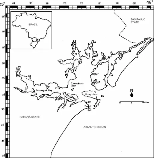
The study area is a tidal flat in Pontal do Sul Resort Beach (Fig. 1), located at the southern entrance to Paranaguá Bay (25o20' - 35'S and 48o20' - 45'W). Due to its geographical location, this tidal flat suffers influence from both the estuarine environment and the adjacent marine environment, presents a shallow slope and forms a narrow sediment strip between the continent and the sea. This environment may be divided into three distinct regions. The first is

always submerged even during low tide and has a sandy to muddy sediment; next, the middle region, is the actual tidal flat, submerged periodically during the high tide and comprises a sandy sediment; the third region remains exposed most of the time and also has a sandy sediment

.

Sampling Design

Fish were collected during the diurnal high tide and diurnal and nocturnal low tides of the syzygial (full moon) and quadrature (waning moon) tides, between August 1998 and July 1999. Two tows were made in the same direction as the current, at a maximum depth of 1.70 m along a 100 m transect parallel to the tidal flat, separated by a 30 m interval. A 2 m long seine-net of 30.0 m x 2.0 m, with a uniform mesh size of 0.5 cm was used.

Simultaneously with the sampling, water temperature, water salinity, and wave height and wave period were measured. Precipitation and wind intensity were obtained from the Centro de Estudos do Mar - UFPR meteorological station in Pontal do Sul. Fish were identified, then weighed (g), and measured (standard and total length in mm) and, when possible, sex and stage of maturity were noted.

Data Analysis

Samples were grouped by month to analyze temporal variations. A fixed ANOVA model (Sokal & Rohlf, 1995) was applied to examine possible differences between the monthly averages of the physical-chemical parameters and between the monthly averages and those of the groups defined by The Cluster Analysis of the number of species, number of fish, total weight, Margalef’s species richness index, Shannon-Wiener’s diversity index (number and weight) and Pielou’s evenness index (Ludwig & Reynolds, 1988). The data were 4th root transformed and tested for homogeneity of variance (Bartelett’s test) and normality (Kolmogorov-Smirnov’s test) before applying the ANOVA. The test of the Least Significant Difference (LSD) was used to determine which averages were different if there were significant differences (p <0,01 and p <0,05), Kruskal-Wallis’s non parametric statistics was used where any assumption of ANOVA was not met (Sokal & Rohlf, 1995, Conover, 1990).

Hierarchical agglomerative cluster analyses and non-metric multidimensional scaling (MDS) were used to study temporal variation in the species’ composition and abundance registered throughout the twelve months. Species had to comprise 1% or more of the total capture and had to be present in at least 6 months for inclusion in the analysis. Numerical occurrence values of these species were 4th root transformed and a similarity matrix was produced using the Bray-Curtis similarity measure, obtaining a cluster using the unweighted pair-group mean arithmetic linking method (UPGMA) (Ludwig & Reynolds, 1988).

The analysis of similarity of percentages (SIMPER) was used to identify the main species responsible for the similarities within each group (most common species) defined by the Cluster Analysis and for the dissimilarities among those groups (most discriminating species). The BIOENV routine was used to examine which environmental variables or group of environmental variables best explained the observed biological patterns (Clarke & Warwick, 1994). The seasons were defined as: September to November = spring; December to February = summer; March to May = autumn; June to August = winter.

R

Environmental Parameters

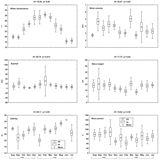
All environmental variables presented significant temporal variation. Temperatures were significantly greater from the beginning of summer to the beginning of autumn, and lower in winter and in September, with the lowest temperatures occurring in June and July (Fig. 2). Average rainfall varied little, with the exception of September, when the average was greater than that in August, October and November. The greatest rainfall occurred in January, February, March and September (Fig. 2). Salinity was highest in May and June, with June presenting the highest average salinity (35), and lower in January, September and October, with January displaying the lowest average salinity (22) (Fig. 2).

The weakest winds were registered in January and February and between April and August, the latter with the smallest average speed (2.7 m/s). Stronger winds occurred between September and December and in March, the latter with the largest average speed (5.1 m/s) (Fig. 2). The smallest waves occurred in February and April and the highest waves occurred in March and between May and November (which did not differ within this group), with intermediary ones in January and December (Fig. 2). Larger wave periods were registered during the spring, with the maximum in October and November (88.4 s and 88.6 s), while the smallest wave periods occurred during the summer, with February presenting the smallest average (42.9s) (Fig. 2).

Ichthyofauna

H= 79,06 p= 0,00

o C

16 18 20 22 24 26 28 30 32

Water temperature

H= 45,97 p= 0,00

m/s

1 2 3 4 5 6 7

Wind velocity

H= 20,78 p= 0,013

mm

-60 -40 -20 0 20 40 60 80 100 120

Rainfall

H= 17,75 p= 0,04

cm

-5 5 15 25 35 45 55 65

Wave height

H= 60,11 p= 0,00

‰

14 18 22 26 30 34 38

Aug Sep Oct Nov Dec Jan Feb Mar Apr May Jun Jul Salinity

±S ±e Mean

[___________1998____________] [________________1999 ________________]

H= 10,62 p= 0,30

s

0 20 40 60 80 100 120 140 160

Aug Sep Oct Nov Dec Jan Feb Mar Apr May Jun Jul ±S

±e Mean Wave period

[___________1998____________] [________________1999 ________________]

Fig. 2. Monthly values of water temperature, rainfall, salinity, wind intensity, wave height and wave period, during the sampling period at the Pontal do Sul Resort Beach tidal flat.

Temporal Variation

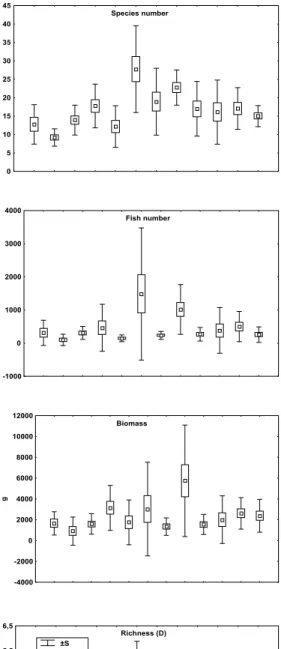
The average number of species, number of fish, biomass and the monthly average species’ richness, species diversity (weight) and evenness showed significant variation during the sample period (Fig. 3, Tab. 2). The average number of species decreased from the maximum in January to the minimum in September. No difference was observed

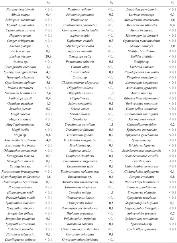
Table 1. List of species of Pontal do Sul Resort Beach tidal flat (% total capture).

% % %

Narcine brasiliensis < 0,1 Pontinus rathbuni < 0,1 Isopisthus parvipinnis < 0,1

Albula vulpes 0,4 Prionotus punctatus 0,2 Larimus breviceps 0,1

Echiopsis intertinctus < 0,1 Prionotus sp. < 0,1 Menticirrhus americanus 1,6

Myrophis punctatus < 0,1 Centropomus parallelus < 0,1 Menticirrhus littoralis 0,4

Cynoponticus savana < 0,1 Centropomus undecimalis < 0,1 Menticirrhus sp. < 0,1

Hoplunni tenuis < 0,1 Alphestes afer < 0,1 Micropogonias furnieri < 0,1

Conger orbignyanu < 0,1 Diplectrum radiale 0,3 Ophioscion punctatissimus < 0,1

Anchoa lyolepis 1,3 Mycteroperca rubra < 0,1 Stellifer rastrifer 3,0

Anchoa parva 0,1 Rypticus randalli < 0,1 Stellifer brasiliensis < 0,1

Anchoa tricolor 29,9 Synagrops bella < 0,1 Stellifer stellifer < 0,1

Anchoa sp. < 0,1 Pomatomus saltatrix 0,1 Stellifer sp. < 0,1

Cetengraulis edentulus 1,2 Caranx latus < 0,1 Umbrina canosai < 0,1

Lycengraulis grossidens 4,7 Caranx ruber 0,1 Pseudupeneus maculatus < 0,1

Harengula clupeola 9,3 Caranx sp. < 0,1 Pinguipes brasilianus < 0,1

Opisthonema oglinum 5,8 Chloroscombrus chrysurus 0,1 Astroscopus sexpinosus < 0,1

Pellona harroweri < 0,1 Oligoplites saliens < 0,1 Astroscopus ygraecum < 0,1

Sardinella brasiliensis 2,4 Oligoplites saurus 1,0 Astroscopus sp. < 0,1

Cathorops spixii 0,4 Oligoplites sp. < 0,1 Ribeiroclinus eigenmanni < 0,1

Genidens genidens 1,5 Selene setapinnis 0,1 Bathygobius soporator < 0,1

Synodus foetens 0,2 Selene vomer 0,1 Gobionellus oceanicus < 0,1

Mugil curema < 0,1 Seriola lalandi < 0,1 Gobionellus smaragdus < 0,1

Mugil curvidens < 0,1 Seriola sp. < 0,1 Microgobius meeki < 0,1

Mugil gaimardianus 0,1 Trachinotus carolinus 1,1 Chaetodipterus faber 0,2

Mugil incilis < 0,1 Trachinotus falcatus 0,9 Sphyraena barracuda < 0,1

Mugil sp. 0,6 Trachinotus goodei 0,2 Sphyraena guachancho < 0,1

Atherinella brasiliensis 4,9 Trachinotus marginatus < 0,1 Sphyraena sp. < 0,1

Austroatherina incisa < 0,1 Trachinotus sp. 0,4 Trichiurus lepturus < 0,1

Odontesthes bonariensis < 0,1 Lutjanus analis < 0,1 Scomberomorus brasiliensis < 0,1

Strongylura marina 0,3 Diapterus rhombeus 0,1 Scomberomorus cavalla < 0,1

Strongylura timucu 0,1 Eucinostomus argenteus 2,7 Peprilus paru < 0,1

Strongylura sp. < 0,1 Eucinostomus gula 0,2 Citharichthys arenaceus < 0,1

Parexocoetus brachypterus < 0,1 Eucinostomus melanopterus < 0,1 Citharichthys spilopterus 0,1

Hyporhamphus unifasciatus 1,6 Eucinostomus sp. 0,6 Etropus crossotus 0,8

Hemiramphus brasiliensis 0,3 Anisotremus surinamensis 16,9 Paralichthys brasiliensis < 0,1

Poecilia vivipara < 0,1 Anisotremus virginicus < 0,1 Trinectes paulistanus < 0,1

Hippocampus reidi < 0,1 Conodon nobilis 1,3 Symphurus plagusia < 0,1

Pseudophallus mindi < 0,1 Genyatremus luteus < 0,1 Symphurus tesselatus < 0,1

Syngnathus dunckeri < 0,1 Orthopristis ruber 0,5 Stephanolepsis hispidus 0,1

Syngnathus elucens < 0,1 Pomadasys corvinaeformis 0,1 Lagocephalus laevigatus < 0,1

Syngnathus folletti < 0,1 Diplodus argenteus < 0,1 Sphoeroides greeleyi 0,2

Syngnathus pelagicus 0,1 Polydactylus virginicus < 0,1 Sphoeroides testudineus 0,1

Syngnathus rousseau < 0,1 Bairdiella ronchus 0,1 Sphoeroides sp. < 0,1

Fistularia petimba < 0,1 Ctenosciaena gracilcirrhus < 0,1 Cyclichthys spinosus < 0,1

Fistularia tabacaria 0,1 Cynoscion leiarchus 0,1

0 5 10 15 20 25 30 35 40 45

Species number

0,2 0,6 1,0 1,4 1,8 2,2 2,6

Diversity (number)

-1000 0 1000 2000 3000 4000

Fish number

0,8 1,0 1,2 1,4 1,6 1,8 2,0 2,2 2,4 2,6

Diversity (weight)

g

-4000 -2000 0 2000 4000 6000 8000 10000 12000

Biomass

0,1 0,2 0,3 0,4 0,5 0,6 0,7 0,8 0,9 1,0

Aug Sep Oct Nov Dec Jan Feb Mar Apr May Jun Jul ±S ±e Mean Evenness (J)

[___________1998____________] [_________________1999 _________________]

0,5 1,5 2,5 3,5 4,5 5,5 6,5

Aug Sep Oct Nov Dec Jan Feb Mar Apr May Jun Jul Richness (D)

±S ±e Mean

[___________1998____________] [_________________1999 _________________]

Species richness peaked in January, then decreased to the lowest in September. It varied during winter and spring, but did not differ statistically among those months (Fig. 3, Tab. 2). Fish weight diversity (Shannon – Wiener) was lower in September and December, and did not vary from the middle of summer to the end of winter. Evenness was greater in September, and lowest in March and October. In comparison to the other seasons, the evenness seems to be larger from the end of autumn to the beginning of spring (Fig. 3, Tab. 2).

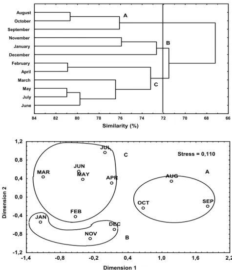
Faunistic similarity between months (combined samples) was analyzed through Cluster and non metric MDS methods. The resulting dendrogram separated the 12 months of collection into three groups connected by 72% or greater similarities (Fig. 4). Group "A", includes August, September and October, with 76% similarity; these months had the lowest average number of species, lowest number of fish and biomass and the lowest richness. Group "B", comprising November, December and January, showed a 73% similarity, with larger number of species, fish number and biomass and a highest richness than observed in group "A". Group B however, did not differ statistically from group "C" (February, March, April, May, June and July), which were 73% similar. Group "C" is formed by two sub-groups, one that joins February and April with 81% similarity, and another with 77% similarity for March, May, June and July (Fig. 4). Clustered samples separation, in the MDS, by month, corresponds to the Cluster analysis pattern (Fig. 4).

The similarity percentages analysis (SIMPER), showed the largest average similarity within group "A" defined by the Cluster analysis (78%), the main contribution to which was by the

species A. tricolor, L. grossidens, H. unifasciatus and E. crossotus (36%) (Tab. 3). The species A. tricolor, H. clupeola, A. surinamensis and S. rastrifer were responsible for the average similarity in group "B" of the Cluster analysis ( 74%). In group "C" the average similarity was 76%, and the species most responsible were A. tricolor, L. grossidens, H. clupeola and A. surinamensis ( 27%). SIMPER also showed a larger dissimilarity between groups "A" and "B" (33%), to which the species A. tricolor, Cetengraulis edentulus, A. brasiliensis and S. rastrifer contributed most (29%). The species H. clupeola, O. oglinum, Genidens genidens, A. surinamensis and Conodon nobilis (35%) were the most responsible for the dissimilarity between groups "A" and "C" (32%). Between groups "B" and "C", the dissimilarity was of 28%, with a larger contribution of the species Anchoa lyolepis, A. tricolor, C. edentulus, O. oglinum, E. argenteus and S. rastrifer (36%) (Tab. 3).

The most numerically dominant species presented an apparent temporal pattern. Cluster analysis, based on abundances of the 27 selected species, separated the species into five groups, united with 74% similarity (Fig. 5). Group "A", which included the species A. tricolor, A. surinamensis and H. clupeola, the most abundant species in the samples and present in all seasons, included juveniles and adults. At 78% similarity group "B" was formed, comprising juveniles and adults from the species L. grossidens, H. unifasciatus, E. crossotus and M. americanus, united at 82% similarity, and the sub-group of the species A. brasiliensis and E. argenteus, joined at the level of 83%, also present in the area in the juvenile and adult stages and presenting high occurrences in all seasons, although with fewer individuals than in the previous group. A third group

Table 2. Result of Variance Analysis (F) and of e Kruskal-Wallis test (H) at Pontal do Sul Resort Beach tidal flat. (NS non-significant difference, ** significant difference at the level of p <0.01, * significant difference at the level of p <0.05).

MONTH GROUP

F p H p F p H p

Number of species 36,61 0,00 ** 11,36 0,00 **

Number of individuals 21,53 0,012 * 1,58 0,45 NS

Biomass 3,46 0,00 ** 6,80 0,03 *

Richness 21,16 0,012 * 10,98 0,00 **

Diversity (number) 4,73 0,85 NS 0,27 0,87 NS

Diversity (weight) 2,68 0,00 ** 0,10 0,95 NS

Similarity (%) June

July May March April February December January November September October August

84 82 80 78 76 74 72 70 68 66

A

B

C

Dimension 1

Dimension 2

AUG

SEP OCT

NOV DEC JAN

FEB MAR

APR MAY

JUN

JUL

-1,2 -0,8 -0,4 0,0 0,4 0,8 1,2

-1,4 -0,8 -0,2 0,4 1,0 1,6 2,2

A

B

C Stress = 0,110

Fig. 4. Dendrogram and ordination by the MDS method based on the density data of the main 27 taxa, at the Pontal do Sul Resort Beach tidal flat. Species groups are delineated at 72% similarity level in the dendrogram, and circle in the ordination plot Ordination MDS stress =0.110.

"C", 78% similar, found throughout the year, included Hemiramphus brasiliensis, S. marina, Menticirrhus littoralis, Oligoplites saurus, T. carolinus and Mugil sp., the first three present in juvenile and adult stages, and only juveniles in the remaining species, with the smallest frequencies in the spring. With 78% similarity, juveniles and adults of the species C. nobilis and G. genidens form group "D", practically absent in the area in the spring and more abundant in the autumn, mainly in March, when there are larger groups of the two species. Finally, group "E" (77% similar) with juveniles and adults of the species Sphoeroides testudineus, Strongylura timucu, Sphoeroides greeleyi and Eucinostomus gula, was present in low numbers in all samples, with larger numbers from spring to the beginning of autumn. The species S. rastrifer did not

Similarity (%) 27. C. edentulus

26. A. lyolepis

25. T. falcatus

24. E. gula

23. S. geeleyi

22. S. timucu

21. S. testudineus

20. G. genidens

19. C. nobilis

18. S.brasiliensis

17. Mugil sp.

16. T. carolinus

15. O. saurus

14. M. littoralis

13. S. marina

12. H brasiliensis

11. E. argenteus

10. A.brasiliensis

9. M. americanus

8. E. crossotus

7. H. unifasciatus

6. L. grossidens

5. S. rastrifer

4. O. oglinum

3. H. clupeola

2. A. surinamensis

1. A. tricolor

95 90 85 80 75 70 65 60 55 50

A

B

C

D

E

Dimension 1

Dimension 2

1 2

6

12

21

7 4

15

18 8

14

3

17 16

9

25

10

13

23

11

22

5

24

19 26

27

20

-2,0 -1,5 -1,0 -0,5 0,0 0,5 1,0 1,5 2,0

-1,6 -1,0 -0,4 0,2 0,8 1,4 2,0

Stress = 0,164

A

B

C D

E

Fig. 5. Dendrogram and ordination by the MDS method showing similarities among the most abundant taxa, based on occurrence, at the Pontal do Sul Resort Beach tidal flat. Species groups are delineated at the 74% similarity level in the dendrogram, and circled in the ordination plot. Ordination MDS stress = 0,164.

In the analysis of the influence of the environmental parameters on the structure of the fish assemblage (BIOENV), low correlation values were obtained (Tab. 4). The maximum correlation occurred with the 2-variable combination wave

Table 3. Percentage contribution (%) of the most abundant and constant species in the tidal flat, for the similarity inside group A (August, September and October), group B (November, December, January) and group C (February, March and April, May, June and July) and for the dissimilarity between these groups (“A” x “B”, “A” x “C”, “B” x “C”).

Table 4. Most significant BIOENV results, indicating wave height (W), wave period (P), salinity (S), water temperature (T), rainfall (R) and wind intensity (I) influence.

T S TI PS TR TS TSI

0,158 -0,121 0,238 -0,286 0,177 0,140 0,249

TRI TRW TRSI TRIP TRSIP TRSIWP

0,229 0,172 0,242 0,190 0,192 0,158

D

A few species were responsible for the largest proportion of the total number of individuals collected at Pontal do Sul tidal flat. This is common in studies of fish populations in shallow bay areas,

estuaries and other coastal environments (Bennett, 1989; Clark et al., 1994; Valesini et al., 1997). In many areas of the Brazilian coast this same pattern has been demonstrated in other shallow environments. (Paiva Filho & Toscano, 1987; Teixeira & Falcão, 1992; Garcia & Vieira, 1997). Among the species that

A B C

Average similarity within each group (%) 78 73 76

Species

Anchoa tricolor 13,17 10,80 6,28

Lycengraulis grossidens 9,22 6,05

Harengula clupeola 6,33 7,70

Hyporhamphus unifasciatus 7,61

Anisotremus surinamensis 6,70 7,41

Stellifer rastrifer 8,22

Etropus crossotus 6,13

A x B A x C B x C

Average dissimilarity between groups (%) 33 32 28

Species

Anchoa lyolepis 5,22

Anchoa tricolor 5,78 7,94

Cetengraulis edentulus 8,21 5,00

Harengula clupeola 6,13

Opisthonema oglinum 6,54 6,74

Genidens genidens 6,30

Atherinella brasiliensis 5,28

Eucinostomus argenteus 4,92

Anisotremus surinamensis 8,61

Conodon nobilis 6,99

dominate in this tidal flat, H. clupeola and A. brasiliensis were dominant in other tidal flat of Paranaguá Bay. (Vendel et.al., 2003).

The general pattern of an increase in the number of species during the spring and summer in the tidal flat of Pontal do Sul was observed in other studies in the southeastern and southern coast of Brazil (Paiva Filho & Toscano, 1987; Giannini & Paiva Filho, 1990; Vendel et.al., 2003). The presence of occasional visitors was greatest in the warmest period of the year, and contributed significantly to the seasonal variation in number of species in the tidal flat.

Despite the greater number of individuals in January and March, mainly due to large aggregates of juveniles of A. tricolor, O. oglinum and A. brasiliensis in January and of A. surinamensis in March, no consistent seasonal tendency was observed throughout the sample period in number of captures. This is explained by large numbers, mainly of juveniles, found in other seasons, for example of A. tricolor and H. clupeola in March, A. tricolor and O. oglinum in June and A. tricolor and S. rastrifer in November, among others. There are no seasonal differences in numbers of fish, yet the studied area has a larger number of fish in summer, autumn and part of winter, a pattern similar to that observed by Vendel et al. (2003) in a tidal flat of the region. On the other hand, Santos et al. (2002) studying two tidal flats in Paranaguá Bay, also did not find any seasonal pattern in the captures in number of fish. In Guaratuba Bay, peaks of fish abundance occurred between the end of autumn and the beginning of winter (Chaves et al., 2000).

Although larger average values of biomass exist for some months of the year, again, no seasonality is readily apparent in biomass. The peak observed in January is due mainly to the captures of many juveniles of A. tricolor and E. argenteus and of adults of S. rastrifer and E. argenteus. The significantly greater average in March is the result, mainly, of captures of juveniles of A. surinamensis, C. nobilis and G. genidens and of adults of S. rastrifer. The increase in the biomass in November was caused by the presence in of large aggregates of juveniles of A. tricolor and adults of A. surinamensis, E. argenteus and S. rastrifer. Despite the absence of a seasonal tendency, the total weight of captures was greater in the tidal flat in the summer, autumn and part of winter, due to the presence of juveniles, in some cases of larger species and of adults.

Species richness showed tendency to increase between the spring and summer, followed by a decreasing over the subsequent months. On average, richness was greatest in summer, autumn and part of winter, a pattern also observed in other tidal flat of Paranaguá Bay (Vendel et al., 2003). Greater species

richness in summer and autumn and lower in winter and spring, were also observed in other study of fish communitie of south Brazil (Monteiro-Neto et al., 1990). Besides the small differences in the number of captured species, with the exception of the high in January and low in June, July, August and September, the large aggregates of some species captured throughout the year contributed to these tendencies. The relationship between the number of captured fish and the number of species, evident in September, does not seem to occur in most months, especially because, the differences in abundance were due mainly to captures of many individuals of few species. Although the capture of individuals and species was much greater in January than in other months, an important part of the species richness is caused by the number of occasional (rare) species.

The Shannon–Wiener diversity index is sensitive to the occurrence of rare species (Peet, 1974). The occurrence of rare (occasional) species followed a seasonal tendency in the tidal flat, but fluctuated widely within seasons, and the same was observed for the species diversity in number and weight. Moreover, diversity reflected the dominance both in number and in weight of a few species. This dominance fluctuated widely within the season, also contributing to the lack of significant seasonal differences. Although the Pielou evenness index is a biased estimator of heterogeneity (by overestimating- Peet, 1974) , again the lack of significant differences among the seasons, reflects the dominance of a few species throughout most of the study period.

Although the groups of selected species are not strongly influenced by seasonality, they are relatively similar to the classification outline proposed by Tyler (1971) for Atlantic coastal communities. According to Tyler’s classification, the Atlantic coastal communities of the United States can be divided into regular components (residents) and periodic components (transients). The periodic components can be winter seasonal, summer seasonal or occasional. In this study the assemblage had regular (groups A, B, C and E) and periodic (group D and the species that did not aggregate) components.

and number of species, indicate the probable importance of these factors in the structuring of the fish assemblage in the tidal flat. In the area, the greatest abundance, biomass and species diversities occurred partly in the periods with higher temperatures, lower salinities, lower wind intensity and lower wave frequencies.

R

Allen, L. G. 1982. Seasonal abundance, composition, and productivity of the littoral fish assemblage in upper Newport Bay, California. Fish. Bull., 80(4):769-790. Bennett, B. A. A. 1989. Comparison of the fish communities

in nearby permanently open, seasonally open and normally closed estuaries in the south – western cape, South Africa. S. Afr. J. Mar., 8:43-55.

Chaves, P. T. C.; Bouchereau, J. L. & Vendel, A. L. 2000. The Guaratuba Bay, Paraná, Brazil (25o52'S; 48o39'W), in the life cycle of coastal fish species. In: INTERNATIONAL CONFERENCE SUSTAINABILITY OF ESTUARIES AND MANGROVES: CHALLENGES AND PROSPECTS. Recife, UFPE. CD-ROM.

Clark, B. M.; Bennett, B. A. & Lamberth, S. J. A. 1994. Comparison of the ichthyofauna of two estuaries and their adjacent surf zones, with an assessment of the effects of beach-seining on the nursery function of estuaries for fish. S. Afr. J. mar. Sci., 14:121-131. Clarke, K. R. & Warwick, R. W. 1994. Change in marine

communities: an aproach to statistical analysis and interpretation. Plymouth Marine Laboratory. 859 p. Conover, W. J. 1990. Practical nonparametric statistics. New

Jersey, John Willey & Sons. 584 p.

Day Jr., J. W.; Hall, C. A. S.; Kemp, W. M. & Yáñez-Arancibia, A. 1989. Estuarine Ecology. New York, John Wiley & Sons. 558p.

Garcia, A. M. & Vieira, J. P. 1997. Abundância e diversidade da assembléia de peixes dentro e fora de uma pradaria de

Ruppia maritima L., no estuário da Lagoa dos Patos (RS,

Brasil). Atlântica, 19:161-181.

Giannini, R. & Paiva Filho, A. M. 1990. Os Sciaenidae (Teleostei - Perciformes) da Baía de Santos (SP), Brasil. Bolm Inst. oceanogr., S Paulo, 38(1):69-86.

Godefroid, R. S.; Hofstaetter, M. & Spach, H. L. 1997. Structure of the fish assemblage in the surf zone beach at Pontal do Sul, Paraná. Nerítica, 11:77-93.

Haendrich, R. L. 1983. Estuarine fishes. In: Ketchum, B. H. ed.. Ecosystems of the World. Amsterdan, Elsevier. p. 183-207.

Hamilton, L. S. & Snedaker, S. C. 1984. Handbook for mangrove area management. Paris, UNESCO. 12: 123 p. Kennish, M. J. 1990. Ecology of estuaries. Boston, CRC.

Press. 391p.

Ludwig, J. A. & Reynolds, J. F. 1988. Statistical ecology. New York. John Wiley & Sons. 337p.

Monteiro-Neto, C.; Blacher, C., Laurent, A. A. S., Snizek, F. N.; Canozzi, M. B. & Tabajara, L. L. C. de A. 1990. Estrutura da comunidade de peixes em águas rasas na região de Laguna, Santa Catarina, Brasil. Atlântica, 12(2):53-69.

Paiva Filho, A. M. & Toscano, A. P. 1987. Estudo comparativo e variação sazonal da ictiofauna na zona entre-marés do Mar Casado - Guarujá e Mar Pequeno - São Vicente, SP. Bolm Inst. ocenogr., S Paulo, 35(2):153-165.

Peet, R. K. 1974. The measurement of species diversity. Annual Review of Ecology and Systematics, 5:285-307. Potter, I. C.; Claridge, P. N. & Warwick, R. M. 1986.

Consistency od seasonal changes in na estuarine fish assemblage. Mar. Ecol. Prog. Ser., 32:217-226. Reise, K. 1985. Tidal flat ecology. Berlin, Spring-Verlag.

191p.

Santos, C.; Schwarz, R.; Oliveira, J. F. & Spach, H. L. 2002. A ictiofauna em duas planícies de maré do setor euhalino da Baía de Paranaguá, PR. B. Inst. Pesca, São Paulo, 28(1): 49-60.

Sokal, R. R. & Rohlf, F. J. 1995. Biometry. New York, W. H. Freeman and Company. 859 p.

Teixeira, R. L. & Falcão, G. A. F. 1992. Composição da fauna nectônica do complexo lagunar Mundaú/ Manguaba, Maceió – AL. Atlântica, 4:43-58.

Tyler, A. V. 1971. Periodic and resident components in communities of Atlantic fishes. J. Fish. Res. Bd. Can., 28:935-946.

Valesini, J. F.; Potter, I. C.; Platell, M. E. & Hyndes, G. A. 1997. Ichthyofaunas of a temperate estuary and adjacent marine embayment. Implications regarding choice of nursery area and influence of environmental changes. Mar. Biol., 128:317-328.

Vendel, A. L.; Lopes, S. B.; Santos, C. & Spach, H. L. 2003. Fish assemblages in a tidal flat. Braz. Arch. Biol. and Tech., 46(2): 233-242.