RAC, Rio de Janeiro, v. 21, n. 6, art. 6, pp. 851-874, Novembro/Dezembro, 2017 http://dx.doi.org/10.1590/1982-7849rac2017170027
Applicability of Investment and Profitability Effects in Asset
Pricing Models
Márcio André Veras Machado1 Robert Faff2 Suelle Cariele de Souza e Silva1
Universidade Federal da Paraíba1
University of Queensland2
Resumo
Este estudo teve por objetivo investigar se investimento e rentabilidade são precificados e se explicam parcialmente as mudanças dos retornos das ações no mercado de capitais brasileiro, conforme o modelo de cinco fatores de Fama e French (2015). Por meio de regressões em série temporal e em cross-section, observou-se que B/M, momento e liquidez, são associados com os retornos das ações, enquanto que investimento e rentabilidade não apresentaram significância. Observou-se, também, que não existe prêmio por investimento no Brasil. Portanto, motivado pelo desempenho do B/M, do momento e da liquidez para o mercado brasileiro, bem como pelo fraco desempenho da rentabilidade e do investimento, pode-se constatar que o modelo de cinco fatores de Keene e Peterson (2007) apresentou desempenho superior a todos os outros modelos, especialmente quando comparado ao modelo de cinco fatores de Fama e French (2015).
Palavras-chave: modelos de precificação de ativos; rentabilidade; investimento; liquidez.
Abstract
This study aims to investigate whether investment and profitability are priced and if they partially explain the variations of stock returns in the Brazilian stock market, according to the Fama and French’s (2015) five-factor model. By using time series and cross-section regression, we found that book-to-market, momentum and liquidity are associated with stock returns whereas investment and profitability were not significant. We also found that there is no investment premium in Brazil. Therefore, motivated by the importance of B/M, momentum and liquidity to the Brazilian stock market, as well as by the poor performance of profitability and investment, we document that Keene and Peterson’s (2007) five-factor model is superior to all other models, especially the five-factor model by Fama and French (2015).
Introduction
Various models have been developed in search of factors that could improve the explanatory power of the Capital Asset Pricing model (CAPM), as well as capture anomalies in asset pricing. Fama and French (1993) developed the three-factor model, namely market – according to the CAPM – firm size and book-to-market ratio (B/M). Carhart (1997) identified the momentum factor and realised that the three-factor model and the CAPM were unable to explain it (Fama & French, 2004). So Carhart (1997) added momentum to Fama and French’s (1993) three-factor model, thus creating the four-factor model, which produced superior empirical evidence. Keene and Peterson (2007) analysed the importance of liquidity as a risk factor in asset pricing models, and added it to Carhart’s (1997) four-factor model, thus concluding that liquidity is priced and explains part of stock return variations, improving the model’s explanatory power.
Size, book-to-market ratio, momentum and liquidity are some characteristics that influence
companies’ returns. Other characteristics also help explain returns, such as factors associated with expected profitability and a company’s expected investment. Fama and French (2006, 2008, 2015), Hou, Xue and Zhang (2015) and Novy-Marx (2013) identified that profitability is positively related to average return. Fama and French (2006, 2008), Xing (2008) and Chen, Novy-Marx and Zhang (2010) documented the negative relation between company investment and return. In addition, Chen et al. (2010) proposed an alternative three-factor model composed by market, profitability and investment risk factors.
According to Fama and French (2006), the existing literature identifies differences in the average return of stocks associated with book-to-market, profitability and investment risk factors, without simultaneously controlling, however, for the said factors. Fama and French (2015) verified that part of the variation in stock returns is left unexplained by the three-factor model they developed in 1993. Then, motivated by valuation theory (Fama & French, 2006), as well as by empirical evidence documented in the literature about the relation between return and profitability (Novy-Marx, 2013) and return and investment (Cooper, Gulen, & Shill, 2008; Lam & Wei, 2011; Li, Becker, & Rosenfeld, 2012; Lipson, Mortal, & Shill, 2011; Watanabe, Xu, Yao, & Yu, 2013; Xing, 2008), Fama and French (2015) and Hou et al. (2015) added profitability and investment factors to the traditional asset pricing models.
Fama and French (2015) added profitability and investment factors to their three-factor model, thus creating a five-factor model. As main results, they found that the five-factor model performed better than the three-factor model. In addition, they observed that model performance was not sensitive to the way factors were constructed. Finally, just like Xing (2008), Fama and French (2015) verified that, by adding profitability and investment factors, B/M factor turned out to be redundant in explaining returns.
Hou et al. (2015) added profitability and investment to market and size factors, thus creating an alternative four-factor model. Aiming to assess the performance of the said model, they compared the performance of the proposed model to that of the three-factor model by Fama and French (1993) as well as that of the four-factor model by Carhart (1997), to explain 80 anomalies documented in the literature. Hou et al. (2015) found that the proposed model performed better than the three-factor and four-factor models in explaining several of the significant anomalies.
The analysis of the joint performance of investment and profitability in stock returns – as well as the use of such variables as risk factors in asset pricing models – in developing countries has been rare. In addition, the findings by Griffin (2002) do not support the notion that it is beneficial to extend multi-factor models to a global context; rather, the specific country should be taken into consideration.
This paper contributes to the literature on multi-factor models by offering international evidence outside the U.S. of the applicability of investment and profitability as risk factors in asset pricing models, especially in a developing country, as is the case of Brazil, whose capital market is the most developed among Latin American countries. Moreover, the five-factor model expands the CAPM model — which is a single-factor model commonly adopted to estimate stock returns — as it adds investment and profitability risk factors, and it better explains stock return variations. This paper also contributes by providing support to researchers and capital market professionals to choose the most appropriate pricing model. By using a model that better explains stock return variations, researchers and market professionals will have a better estimate of the firm’s capital cost for capital budgeting and stock assessment; it may also be used to estimate expected returns, to assess the performance of mutual funds, and to analyse market efficiency. Finally, more empirical researches that demonstrate the applicability and performance of alternative models in markets other than the U.S.A. allow proving that alternative models are superior (or, perhaps, that they are not superior) to the traditional ones, not only in the U.S. market but also in the international spectrum (Amman, Odoni, & Oesch, 2012).
Empirical evidence of multi-factor models both in the U.S. and in the international market suggests that a great part of returns is still left unexplained (Fama & French, 2015; Hou, Xue, & Zhang, 2015; Walkshäusl & Lobe, 2014). Thus, new models that add new factors and use new methodological constructions are welcome. Consequently, this study also contributes to the literature by using a liquidity factor, which was not taken into consideration in Fama and French (2015) or Hou et al. (2015), although it was found to be fundamental in the Brazilian market (Machado & Medeiros, 2011). Although the models by Fama and French (2015) and Hou et al. (2015) have a common focus, namely the inclusion of profitability and investment factors, they differ when it comes to implementation. They also reach inconclusive results, which justifies the need for additional empirical evidence, mainly outside the U.S. market, where said models were developed. Finally, this study intends to compare the performance of the five-factor model by Fama and French (2015) with the five-factor model applied in Brazil by Machado and Medeiros (2011), which performed better than the other pricing models.
There are five sections after this introduction. The next section presents data, variables and
summary statistics. Then, we addresses empirical analysis and results, as well as the outlines the model’s
performance. The next section presents a further analysis and, finally, the conclusions.
Data, Variables and Summary Statistics
Data used in this study were collected from Economatica, a data base largely used in Brazil, which contains accounting and market information of the companies listed at B3 (Brasil, Bolsa e Balcão). Data includes companies that are both active and inactive in the capital market, in order to avoid survivor bias. The sampled period chosen was 1 June 1997 to 30 June 2014. The year 1997 was chosen since the operationalisation of some variables use data related to two previous years, which culminates in using data from 1995. Data prior to 1995 in Brazil are affected by high inflation and lack of currency standardisation.
the latter is influenced by their high degree of leverage; (b) firms that did not present market value set on 31 December and 30 June of each year, for these values serve to compute the book-to-market ratio and company size; (c) firms that presented negative equity on 31 December of each year, as this affects book-to-market ratio; (d) firms that did not have monthly quotations for 24 consecutive months, 12 months prior or 12 months after portfolio formation, considering that this procedure reduces the influence of small-sized and young firms in the results (Anderson & Garcia-Feijó, 2006); and, (e) firms that did not present information concerning accounting data.
Data of 188 stocks (48% of the population), on average, were analysed per year. The year 2003 presented a minimum of 98 stocks (27% of the population) and 2012 a maximum of 266 stocks (69% of the population). The size of this sample is satisfactory, compared to other studies, mainly international studies that used Brazilian stock data. Machado and Medeiros (2011) and Walkshäusl and Lobe (2014) analysed, on average, 149 and 178 stocks per year, respectively. As to market capitalisations, in the 1997-2013 period, the sample corresponded to a minimum of 54% in 1998 and a maximum of 94% in 2010. In this study sample, 48% of the companies represent 85% of market capitalisation in the analysed period.
The explanatory variables analysed were size, B/M, momentum, liquidity, investment and profitability and the Table 1 shows the summary statistics. Specifically, size (ME) is the market equity (price times shares outstanding) by the end of June of year t. B/M is the book value of the Equity in December of year t-1 divided by the market value of Equity in December of year t-1. Momentum (RET11) is the accumulated return in the 11-month period, starting July of year t-1 and finishing May of year t. Liquidity (LIQ) is the negotiated volume, represented by the annual average volume negotiated, in Brazilian Reais, for the stock in the period from July of year t-1 to June of year t, according to the suggestion of Machado and Medeiros (2011). Profitability (E/A) is calculated as Earning Before Interest and Taxes (EBIT) of year t-1 divided by the operational asset of year t-1. Investment (INV) is the change in total asset between years t-2 and t-1 divided by the total asset of year t-2. Variables were measured at company level, following the orientation by Aharoni, Grundy and Zeng (2013).
Table 1
Summary Statistics for the Explanatory Variables
Variable ME B/M RET11 LIQ E/A INV
Average 4,123 1.24 0.11 205 0.10 1.98
SD 14,320 1.68 0.53 920 0.27 94.15
25th 126 0.41 - 0.17 1 0.03 0.01
Median 645 0.80 0.12 9 0.09 0.09
75th 3,054 1.43 0.38 93 0.17 0.21
CV 3.47 1.36 4.82 4.49 2.7 47.55
Note. This table shows the summary statistics for the explanatory variables, including average, standard deviation, 25th percentile, median, 75th percentile and the coefficient of variation (CV). Size (ME) is the market equity (price times shares outstanding) by the end of June of year t. B/M is the book value of Equity in December of year t-1 divided by the market value of the Equity in December of year t-1. Momentum (RET11) is the accumulated return in the 11-month period starting July of year t-1 and finishing May of year t. Liquidity (LIQ) is the negotiated volume, represented by the annual average volume negotiated, in Brazilian Reais, for the stock in the period from July of year t-1 to June of year t. Investment (INV) is the change in total asset between years t-2 and t-1 divided by the total asset of year t-2. Profitability (E/A) is calculated as Earning Before Interest and Taxes (EBIT) of year t-1 divided by the operational asset of year t-1.
Empirical Analysis and Results
Returns to sorted portfolios
Aiming to know, initially, how variables drive the variation of returns, stocks were grouped according to a characteristic of interest (explanatory variable). Table 2 shows the average monthly return for the quintiles formed on size, B/M, momentum, liquidity, investment and profitability variables. Specifically, by the end of June of each year t, stocks were arranged in ascending order according to the variable of interest (size, B/M, momentum, liquidity, investment and profitability). They were sorted into five portfolios based on the quintile breakpoints. From July of year t to June of year t+ 1, the average monthly value-weighted return of each portfolio was calculated. The portfolios were rebalanced annually, by the end of June of each year.
Table 2
Average Monthly Return of Portfolios Formed on Size, Book-to-Market, Momentum, Liquidity, Investment and Profitability
Low 2 3 4 High H-L
Panel A: Student’s t-test
Size-based portfolios 0.012** 0.019*** 0.014** 0.017*** 0.014** 0.002
B/M-based portfolios 0.023*** 0.017*** 0.009 0.005 -0.002 -0.025***
Momentum-based portfolios -0.006 0.010 0.015** 0.021*** 0.031*** 0.037***
Liquidity-based portfolios 0.033*** 0.020*** 0.021*** 0.014** 0.012** -0.021**
Profitability-based portfolios 0.015** 0.009 0.015** 0.015** 0.018*** 0.003
Investment-based portfolios 0.017*** 0.007 0.010 0.017*** 0.014** -0.003
Panel C: Wilcoxon test
Size-based portfolios 0.012*** 0.019*** 0.014*** 0.017*** 0.014*** 0.002
B/M-based portfolios 0.023*** 0.017*** 0.009** 0.005* -0.002 -0.025***
Momentum-based portfolios -0.006 0.010** 0.015*** 0.021*** 0.031*** 0.037***
Liquidity-based portfolios 0.033*** 0.020*** 0.021*** 0.014*** 0.012*** -0.021
Profitability-based portfolios 0.015*** 0.009** 0.015*** 0.015*** 0.018*** 0.003
Investment-based portfolios 0.017*** 0.007** 0.010*** 0.017*** 0.014*** -0.003
Note. By the end of June of each year t, stocks were arranged in ascending order according to the variable of interest (size,
B/M, momentum, liquidity, investment and profitability). They were sorted into five portfolios based on the quintile breakpoints. From July of year t to June of year t+ 1, the average monthly value-weighted return of each portfolio was calculated. All variables are defined in section Data, Variables and Summary Statistics.
*** p-value <0.01, ** p-value <0.05, * p-value<0.10.
Table 2 shows that the average monthly returns of the spread portfolios are statistically significant
companies with the worst accumulated returns in the last 11 months, generating a premium of 3.7% per month (p-value < 0.01). Finally, portfolios formed by low-liquidity companies reach superior returns to the portfolios formed by high-liquidity stocks, generating a premium of 2.1% per month (p-value < 0.05). These results also ratify previous results obtained in Brazil for the aforementioned variables (Machado & Medeiros, 2011, 2012).
Table 2 also shows that for size, profitability and investment, the average monthly returns of the spread portfolios are not statistically significant, according to parametric and non-parametric tests, although they present the expected sign, except for size, considering that more profitable companies present higher average monthly return than less profitable companies. Table 2 also evidences that more conservative companies, in terms of investments, showed a higher average monthly return than companies that invest more, and that bigger companies had superior return to smaller companies. Therefore, since the five-factor model of Fama and French (2015) includes profitability and investment as risk factors, this can be interpreted as the first sign of the model's poor capacity to explain stock returns in the Brazilian market. On the other hand, it signals a possible superiority of the model that contains B/M, momentum and liquidity risk factors.
Another issue was observed: the behaviour of the average returns of the portfolios formed on the combination of size, B/M, profitability and investment, which served as a basis to analyse the performance of multi-factor models (section Model Performance). Table 3, Panel A, shows the average value-weighted returns of the 25 portfolios constructed on the combination of five groups of size and five groups of B/M ratio (5 x 5). In each column of Panel A of Table 3 what can be seen is the size effect while the value effect can be seen on each line. Only in the first column (low B/M) can the size effect be seen; companies of lower market value have higher average returns when compared to companies of higher market value. Therefore, growth companies (low B/M) of low market value reach superior average return to growth companies of high market value. There is no evidence of B/M effect, since all returns related to the high column are lower than the returns in the low column, which ratifies the results of Table 3.
Table 3
Average Monthly Returns of Portfolios Formed on Size, Book-to-Market, Investment and Profitability
Panel A: 5 x 5 portfolios formed on size and B/M
Low 2 3 4 High
Small 0.026 0.017 0.011 0.006 -0.008
2 0.026 0.029 0.015 0.012 -0.003
3 0.018 0.025 0.015 0.004 -0.006
4 0.031 0.020 0.014 0.012 0.003
Big 0.020 0.022 0.011 0.011 -0.001
Panel B: 2 x 4 x 4 portfolios formed on size, B/M and profitability
Small Big
B/M Low 2 3 High B/M Low 2 3 High Low E/A 0.034 0.020 0.008 -0.005 Low E/A 0.016 0.015 0.014 -0.001
2 0.028 0.022 0.006 -0.006 2 0.024 0.020 0.004 -0.004
3 0.028 0.020 0.008 0.000 3 0.020 0.018 0.005 0.001
High E/A 0.026 0.017 0.001 -0.003 High E/A 0.020 0.020 0.003 0.002
Table 3 (continued)
Panel C: 2 x 4 x 4 portfolios formed on size, B/M and investment
Small Big
B/M Low 2 3 High B/M Low 2 3 High Low Inv 0.028 0.016 0.000 -0.002 Low Inv 0.026 0.023 0.015 -0.001
2 0.028 0.028 0.013 0.001 2 0.019 0.026 0.006 -0.003
3 0.030 0.017 0.012 0.001 3 0.021 0.016 0.012 0.000
High Inv 0.022 0.012 0.003 -0.016 High Inv 0.025 0.009 0.004 -0.003
Note. Panel A shows the average value-weighted monthly returns of the 25 portfolios constructed from the combination of five
size groups and five B/M ratio groups. Panel B shows the average value-weighted monthly returns of the 32 portfolios constructed from the combination of two size groups, four B/M ratio groups and four profitability-related groups. Panel C presents the average value-weighted monthly returns of the 32 portfolios constructed from the combinations of the two size groups, four B/M ratio groups and four investment-related groups.
Panel B of Table 3 shows the average returns of the 32 portfolios constructed on the combination of two size groups, four B/M ratio groups and four profitability-related groups. Each column of Panel B of Table 3 shows profitability effect and each line shows value effect. Regardless of the company size, the B/M effect is contrary to what was expected, since all returns related to the high column are lower than the returns in the low column, which ratifies previous results. To companies of high market value, except for the third quartile (in the column), the average returns of more profitable companies is superior to those of less profitable companies, which suggests evidence of a profitability effect. Yet, for companies of low market value, a profitability effect can be observed only when the company has a high B/M ratio.
Panel C of Table 3 shows the average returns of 32 portfolios constructed on the combination of size, B/M and investment variables. These portfolios were constructed the same way as the portfolios for Panel B; only the third variable (profitability) was substituted for by the variable investment. Just like Panel B, regardless of the company size, the B/M effect is contrary to what was expected. For companies of high market value, in all quartiles (in the column), the average returns of companies that invest less is superior to those of companies that invest more, which suggests evidence of investment effect. For companies of low market value, however, investment effect is seen only in the first two quartiles (in the column).
Predictability of returns
Variables that produce great spreads in portfolios’ average returns are candidates for common risk factors. However, those variables that are used to construct portfolios and, consequently, calculate spreads may not be associated with average returns. Therefore, it is necessary to examine if the variables used in asset pricing models (Equations 2 to 7) explain average returns. For this reason, the approach by Fama and MacBeth (1973) was adopted to estimate the coefficients of interest in Equation 1.
INV E/A
+ L 11 +
ME + =
Rett
1 t
2BMt
3RET t
4 IQt
5 t
6 t
t (1)Where:
Before Interest and Taxes (EBIT) of year t-1 divided by the operational asset of year t-1. Investment (INV) is the change in total asset between years t-2 and t-1 divided by the total asset of year t-2.
The estimation of Equation 1 will provide evidence of the sign of the coefficient of the variables, which must be negative for size, liquidity and investment and positive for B/M, momentum and profitability. In addition, through the stated equations, it is possible to see which variables explain stock average returns.
Table 4 shows the average slopes and the p-value for each variable examined in this study. The annual stock return is regressed on the variables of interest. Regressions are conducted for all, small and big companies. Size groups are defined from the arrangement of companies into two groups (Small and Big), based on the median of the company's market value in June of year t.
Table 4 shows that returns are positively associated with size, momentum and profitability and negatively associated with B/M ratio, liquidity and investment. The sign of the relation between stock returns and company size was not persistent among the models. Meanwhile, the sign of the B/M ratio is persistent and significant in all models; however, it presents the opposite of the expected sign, which ratifies the findings of Tables 1 and 2 and previous empirical evidence (Machado & Medeiros, 2011, 2012). The coefficient associated with B/M ratio ranges from -0.088 (p-value < 0.01) to -0.065 (p-value < 0.01).
Table 4
Fama-MacBeth Regressions of Annual Returns on Determinant Return Variables
Intercept ME B/M RET11 LIQ RENT INV F stat
All 0.335** 0.002 -0.065*** 0.348*** -0.021** 0.085 -0.039 20.46***
Small 0.579*** -0.016 -0.067*** 0.368*** -0.024** 0.101 -0.074 16,48***
Big 0.224 0.007 -0.088*** 0.345*** -0.016 -0.042 -0.061 25,63***
Note. This table shows the average slopes and the coefficients from cross-section regressions. All variables are defined in section Data, Variables and Summary Statistics. Size groups are defined from the arrangement of companies into two groups (Small and Big), based on the median of the company's market value in June of year t.
*** p-value <0.01, ** p-value <0.05, * p-value<0.10.
As to momentum and liquidity, the coefficients have the expected sign, with values of 0.345 (p-value < 0.01) and 0.368 (p-(p-value < 0.01) and -0.024 (p-(p-value < 0.05) and -0.016 (p-(p-value > 0.10), respectively, as well as statistical significance, in all analysed models. Meanwhile, investment and profitability do not influence stock returns, since, in all analysed models, their coefficients did not present statistical significance, although the expected sign was observed. We also verified whether the results found were sensitive to company size, sorting stocks into Small and Big, according to Table 4; the conclusion is that results are qualitatively similar.
Since investment and profitability variables are included as risk factors in Fama and French’s (2015) five-factor model, and it does not add explanatory power to returns, this may be interpreted as the second sign of the model’s poor capacity to explain stock returns in the Brazilian market. On the other hand, ratifying the results of Table 2, in all models, B/M, momentum and liquidity were significant, which indicates a possible superiority of the model containing the said variables as risk factors.
Asset pricing models and factor construction
E(R
)
-
R
+
s(SMB)
(
)
+
=
R
-)
E(R
c,t f,t
b
m,t f,t t
h
HML
t
t (2)
E(R
)
-
R
+
s(SMB)
(
)
(
)
+
=
R
-)
E(R
c,t f,t
b
m,t f,t t
h
HML
t
w
WML
t
t (3)
E(R )-R
+s(SMB) ( ) ( ) ( )+ = R -)
E(Rc,t f,t
b m,t f,t t h HML t wWML t l LMH t
t (4)
E(R
)
-
R
+
(
)
(
)
+
=
R
-)
E(R
c,t f,t
b
m,t f,tr
RMW
t
c
CMA
t
t (5)
E(R
)
-
R
+
s(SMB)
(
)
(
)
+
=
R
-)
E(R
c,t f,t
b
m,t f,t t
r
RMW
t
c
CMA
t
t (6)
E(R
)
-
R
+
s(SMB)
(
)
(
)
(
)
+
=
R
-)
E(R
c,t f,t
b
m,t f,t t
h
HML
t
r
RMW
t
c
CMA
t
t (7)Where:
Rp,t is the portfolio return in month t; Rf,t is the risk-free rate in month t, adopting the Selic rate as
proxy; Rp,t – Rf,t is the excess return of the portfolio; Rm,t is the market return in month t; Rm,t – Rf,t is
market risk premium; SMBt, HMLt, WMLt, LMHt, RMWt and CMAt are, respectively, size,
book-to-market, momentum, liquidity, profitability and investment factors, all in month t; , b, s, h, w, l, r and c are the estimated coefficients in the regressions; and εt is the random error term.
Equation 2 refers to the three-factor model of Fama and French (1993), henceforth called model 1. Equation 3 refers to the four-factor model of Carhart (1997), henceforth model 2. Equation 4 refers to the five-factor model of Keene and Peterson (2007), henceforth model 3. Equation 5 refers to the three-factor model of Chen et al. (2010), henceforth model 4. Equation 6 refers to the adapted four-factor model of Hou et al. (2015), henceforth model 5. Equation 7 refers to the five-four-factor model of Fama and French (2015), henceforth model 6.
Apart from the models presented above, we analysed other asset pricing models constructed from the combination of the factors in model 6. In addition, we tested another five-factor model: it incorporates liquidity factor into the adapted four-factor model by Hou et al. (2015), henceforth called model 7. Two other models were tested: one model combines size with profitability and liquidity, the other model combines size with investment and liquidity.
The choice for analysing stock liquidity together with other variables is due to the fact that liquidity premium exists in Brazil (Machado & Medeiros, 2012); another justification is the superior performance of Keene and Peterson’s (2007) five-factor model in Brazil (Machado & Medeiros, 2011). Tables 1 and 3 ratify the importance of liquidity in the Brazilian market.
Table 5
Construction of Size, Book-to-Market, Profitability, Investment, Momentum and Liquidity Factors
Sort Breakpoints Factors and their components Construction of models 6, 5, 4 and 1
2 x 3 combination of ME and B/M, ME and E/A, ME and INV
ME: median SMBB/M = (SH + SN + SL)/3 – (BH + BN + BL)/3
SMBE/A = (SR + SN + SW)/3 – (BR + BN + BW)/3
SMBINV = (SC + SN + SA)/3 – (BC + BN + BA)/3
SMB = (SMBB/M + SMBE/A + SMBINV )/3
B/M: percentiles
E/A: 30th and 70th percentiles
INV: 30th and 70th percentiles
HML = (SH + BH)/2 – (SL+ BL)/2 RMW = (SR + BR)/2 – (SW + BW)/2 CMA = (SC + BC)/2 – (SA + BA)/2 Construction of models 3 and 2
2 x 3 combination of ME and B/M, ME and MOM, ME and LIQ
ME: median SMBB/M = (SH + SN + SL)/3 – (BH + BN + BL)/3
SMBMom = (SW + SN + SL)/3 – (BW + BN + BL)/3
SMBLIQ = (SH + SN + SL)/3 – (BH + BN + BL)/3
SMB = (SMBB/M + SMBMom+ SMBLIQ )/3
B/M: 30th and 70th percentiles
MOM: 30th and 70th percentiles
LIQ: 30th and 70th percentiles
HML = (SH + BH)/2 – (SL + BL)/2 WML = (SW + BW)/2 – (SL + BL)/2 LMH = (SL + BL)/2 – (SH + BH)/2 Construction of model 7
2 x 3 combination of ME and E/A, ME and INV, ME and LIQ
ME: median SMBE/A = (SR + SN + SW)/3 – (BR + BN + BW)/3
SMBINV = (SC + SN + SA)/3 – (BC + BN + BA)/3
SMBLIQ = (SH + SN + SL)/3 – (BH + BN + BL)/3
SMB = (SMBE/A + SMBINV + SMBLIQ)/3
E/A: 30th and 70th percentiles INV: 30th and 70th percentiles LIQ: 30th and 70th percentiles
RMW = (SR + BR)/2 – (SW + BW)/2 CMA = (SC + BC)/2 – (SA + BA)/2 LMH = (SL + BL)/2 – (SH + BH)/2
Note. Variables were arranged independently in 2 x 3 sets of combinations, where size interacted with the other variables of
interest separately (B/M, E/A, INV, RET11, LIQ). Size breakpoint was the median of the market values of the companies in the sample; for the other variables breakpoints were the 30th and 70th percentiles corresponding to their value. SMB factors (small minus big), HML (B/M-related high minus low), RMW (profitability-related robust minus weak), CMA (investment-related conservative minus aggressive), WML (momentum-(investment-related winner minus loser), LMH (liquidity-(investment-related low minus high). Source: Adapted from Fama, E. F., & French, K. R. (2015). A five-factor asset pricing model. Journal of Financial Economics, 116(1), 1-22. http://dx.doi.org/10.1016/j.jfineco.2014.10.010.
The second and third approaches of factor construction are similar to the first approach; the only difference is the way variables are combined. In the second approach, factors are constructed independently; stocks were sorted in 2 x 2 sets of combinations. Size interacted with the other variables of interest separately. Meanwhile, in the third approach, all variables are jointly controlled and stocks are classified in 2 x 2 x 2 x 2 sets of combinations, where all variables interact with one another. All factors were calculated monthly. The market factor for all models was obtained by the difference between the average monthly value-weighted return of all sample stocks and the risk-free rate; Selic rate was adopted as proxy.
factor was constructed; it was significant only when the factor was set in a 2 x 3 form (size and profitability). Finally, the different versions of the factors are highly correlated, ranging from 0.896 to 0.995 for the SMB factor, from 0.722 to 0.862 for the profitability factor, from 0.793 to 0.822 for the investment factor, from 0.734 to 0.880 for the liquidity factor and from 0.887 to 0.918 for the momentum factor. These results ratify those obtained from Tables 1 and 3, strengthening the evidence that Fama and French’s (2015) five-factor model has a poor capacity to explain stock returns in the Brazilian market, as well as the possible superiority of the model containing B/M, momentum and liquidity as risk factors.
Table 6
Mean for the Monthly Returns of the Factors
Models 6, 5, 4 and 1 Models 3 and 2 2 x 3
Factors
2 x 2 Factors
2 x 2 x 2 x 2 Factors
2 x 3 Factors
2 x 2 Factors
2 x 2 x 2 x 2 Factors Rm - Rf 0.002 0.002 0.002 Rm - Rf 0.002 0.002 0.002
SMB 0.003 0.003 0.003 SMB 0.001 0.002 0.000
HML -0.028*** -0.020*** -0.018*** HML -0.028*** -0.020*** -0.019***
RMW 0.007** 0.004 -0.018 WML 0.029*** 0.019*** 0.015***
CMA 0.000 -0.003 0.001 LMH 0.010** 0.006** 0.005*
Model 7 2 x 3 Factors
2 x 2 Factors
2 x 2 x 2 x 2 Factors Rm - Rf 0.002 0.002 0.002
SMB 0.003 0.003 0.001
RMW 0.007** 0.004 0.004*
CMA 0.000 -0.003 -0.001
LMH 0.010** 0.006** 0.005*
Note. Rm– Rf is the difference between the average monthly value-weighted return of all stocks of the sample and the risk-free rate (Selic); SMB is the size factor; HML is the B/M-based value factor; RMW is the profitability factor; CMA is the investment factor, LMH is the liquidity factor; and WML is the momentum factor. Since VIF values are below 5, there is no collinearity between the variables, in any of the analysed models.
*** p-value <0.01, ** p-value <0.05, * p-value<0.10.
Model Performance
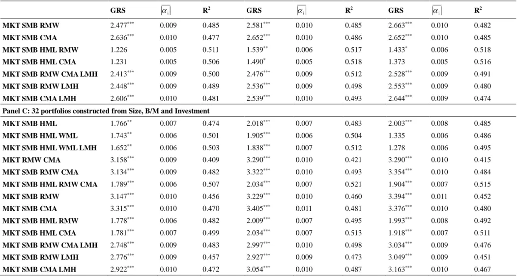
This section assesses how well asset pricing models explain the excess return of three sets of portfolios. Thirteen pricing models were analysed, six of which were proposed by other authors and were duly tested; the remaining models were constructed from the combination of the risk factors analysed in this study. In all, four three-factor models, six four-factor models and three five-factor models were analysed. If pricing models capture all the variation of the expected return, the intercept must be zero for all portfolios. Thus we ran the GRS test proposed by Gibbons, Ross and Shanken (1989), which tests if all estimated intercepts jointly equal zero.
(2015). The aim was to investigate how profitability, investment and liquidity factors improved the description of the returns.
Table 7 shows the GRS test statistic, the average bsolute value of the intercepts (|��|) and the cross-section variation of expected returns explained by the model (adjusted R2). The Panel A, where the dependent variable of the regressions is the return of the portfolios constructed from size and B/M, shows that the model that contains market, size, B/M, momentum and liquidity risk factors (model 3) performed best, according to the GRS statistic, average intercept and adjusted R2. The substitution of momentum and liquidity for profitability and investment considerably worsens the GRS statistic and other statistics, which shows that model 3 is superior to model 6.
Panel A of Table 7 shows that, regardless of the way factors were constructed, the GRS statistic of the model constituted by market, size and B/M (model 1) is very close to the GRS statistic of the model constituted by market, size, B/M, profitability and investment (model 6) as well as to variants of model 6, which excludes one of the factors (profitability or investment). The models that do not have the HML factor are the models that have the highest GRS statistic and the highest absolute intercepts, on average, which suggests that HML is important in the explanation of returns. Therefore, profitability and investment do not aggregate value to most of the models; also, such factors do not substitute for HML. These findings diverge from the result found by Fama and French (2015) in the US market, which showed that the five-factor model (market, size, B/M, profitability and investment) had the lowest GRS statistic, suggesting that it was the least imperfect model in explaining returns, and that it performed better than the three-factor model by Fama and French (1993) as well.
The results shown in Panel A of Table 7 do not change when the returns of the portfolios constructed from size, B/M and investment (2 x 4 x 4) are used as dependent variables, according to Panel C. Results from Panel C show that model 3 captures all variation of the returns of the portfolios, when the factors are constructed as 2 x 2 x 2 x 2, not rejecting the null hypothesis that the intercepts are jointly equal to zero.
Table 7
Summary Statistics for Asset Pricing Models
GRS i R
2 GRS
i
R2 GRS
i
R2
2 x 3 Factors 2 x 2 Factors 2 x 2 x 2 x 2 Factors
Panel A: 25 portfolios constructed from Size and B/M
MKT SMB HML 2.144*** 0.006 0.534 2.434*** 0.007 0.538 2.599*** 0.008 0.531
MKT SMB HML WML 2.092*** 0.006 0.561 2.267*** 0.006 0.561 1.799 0.005 0.539
MKT SMB HML WML LMH 1.969*** 0.005 0.567 2.362*** 0.006 0.574 1.797 0.005 0.553
MKT RMW CMA 3.741*** 0.008 0.437 3.893*** 0.008 0.445 4.072*** 0.008 0.444
MKT SMB RMW CMA 3.726*** 0.008 0.528 3.941*** 0.008 0.540 4.202*** 0.009 0.523
MKT SMB HML RMW CMA 2.139*** 0.006 0.553 2.455*** 0.007 0.567 2.503*** 0.007 0.549
MKT SMB RMW 3.770*** 0.008 0.514 3.959*** 0.008 0.518 4.245*** 0.009 0.497
MKT SMB CMA 3.978*** 0.009 0.520 4.000*** 0.009 0.533 4.168*** 0.009 0.522
MKT SMB HML RMW 2.143*** 0.006 0.540 2.544*** 0.007 0.551 2.614*** 0.008 0.534
MKT SMB HML CMA 2.150*** 0.006 0.548 2.376*** 0.007 0.562 2.497*** 0.007 0.549
MKT SMB RMW CMA LMH 3.325*** 0.008 0.530 3.865*** 0.009 0.549 3.802*** 0.008 0.522
MKT SMB RMW LMH 3.372*** 0.008 0.516 3.949*** 0.009 0.536 3.837*** 0.008 0.511
MKT SMB CMA LMH 3.573*** 0.009 0.522 3.851*** 0.009 0.542 3.913*** 0.009 0.517
Panel B: 32 portfolios constructed from Size, B/M and Profitability
MKT SMB HML 1.239 0.005 0.494 1.542** 0.006 0.501 1.438* 0.006 0.503
MKT SMB HML WML 1.382 0.005 0.518 1.573** 0.005 0.514 1.032 0.005 0.494
MKT SMB HML WML LMH 1.603*** 0.005 0.524 1.805*** 0.005 0.523 1.146 0.005 0.503
MKT RMW CMA 2.483*** 0.009 0.427 2.569*** 0.010 0.437 2.657*** 0.010 0.431
MKT SMB RMW CMA 2.446*** 0.009 0.496 2.569*** 0.010 0.506 2.633*** 0.010 0.498
MKT SMB HML RMW CMA 1.217 0.005 0.522 1.477* 0.005 0.532 1.361 0.005 0.528
Table 7 (continued)
GRS i R
2 GRS
i
R2 GRS
i
R2
MKT SMB RMW 2.477*** 0.009 0.485 2.581*** 0.010 0.485 2.663*** 0.010 0.482
MKT SMB CMA 2.636*** 0.010 0.477 2.652*** 0.010 0.486 2.652*** 0.010 0.485
MKT SMB HML RMW 1.226 0.005 0.511 1.539** 0.006 0.517 1.433* 0.006 0.518
MKT SMB HML CMA 1.231 0.005 0.506 1.490* 0.005 0.518 1.373 0.005 0.516
MKT SMB RMW CMA LMH 2.413*** 0.009 0.500 2.476*** 0.009 0.512 2.528*** 0.009 0.491
MKT SMB RMW LMH 2.448*** 0.009 0.489 2.536*** 0.009 0.498 2.553*** 0.009 0.480
MKT SMB CMA LMH 2.606*** 0.010 0.481 2.539*** 0.010 0.493 2.644*** 0.009 0.474
Panel C: 32 portfolios constructed from Size, B/M and Investment
MKT SMB HML 1.766** 0.007 0.474 2.018*** 0.007 0.483 2.003*** 0.008 0.485
MKT SMB HML WML 1.743** 0.006 0.501 1.905*** 0.006 0.504 1.335 0.006 0.486
MKT SMB HML WML LMH 1.652** 0.006 0.503 1.838*** 0.007 0.512 1.278 0.006 0.495
MKT RMW CMA 3.158*** 0.009 0.409 3.290*** 0.010 0.421 3.290*** 0.010 0.415
MKT SMB RMW CMA 3.134*** 0.009 0.482 3.322*** 0.010 0.493 3.354*** 0.010 0.484
MKT SMB HML RMW CMA 1.789*** 0.006 0.507 2.034*** 0.007 0.521 1.904*** 0.007 0.515
MKT SMB RMW 3.147*** 0.010 0.456 3.229*** 0.010 0.460 3.394*** 0.011 0.452
MKT SMB CMA 3.315*** 0.010 0.470 3.405*** 0.011 0.481 3.376*** 0.010 0.480
MKT SMB HML RMW 1.778*** 0.006 0.482 2.009*** 0.007 0.495 1.993*** 0.008 0.492
MKT SMB HML CMA 1.781*** 0.007 0.499 2.034*** 0.007 0.513 1.918*** 0.007 0.511
MKT SMB RMW CMA LMH 2.748*** 0.009 0.483 2.997*** 0.010 0.498 3.034*** 0.009 0.476
MKT SMB RMW LMH 2.776*** 0.009 0.457 2.927*** 0.009 0.473 3.049*** 0.009 0.451
MKT SMB CMA LMH 2.922*** 0.010 0.472 3.054*** 0.010 0.487 3.163*** 0.010 0.467
Note. This table shows statistics of the GRS test, the probability (p-value) of the GRS statistic, the average absolute value of the intercepts (
i
All this considered, results obtained from Table 7 confirm the preliminary results obtained from Tables 2, 4 and 6, namely the poor ability of Fama and French’s (2015) five-factor model to explain stock returns in the Brazilian market and the possible superiority of Keene and Peterson’s (2007) five-factor model, which uses market, size, B/M, momentum and liquidity as risk five-factors. These results are due to the poor performance of profitability and investment and to the good performance of B/M, momentum and liquidity.
Further Analysis
Are book-to-market, momentum and liquidity redundant factors in Brazil?
Fama and French (2015) found that HML is a redundant factor in describing average returns in their five-factor model. They recommend an investigation into this behaviour, to examine if it can be observed in international markets. Although the results of the models performance do not support the suspicion that HML is a redundant factor in Brazil, we aimed to verify if HML is a redundant factor with profitability and investment, as suggested by Fama and French (2015). To verify if this result is common in Brazil, we regressed each of the factors in the five-factor model by Fama and French (2015) on the other four remaining factors. Table 8 shows the estimated parameters in the regressions.
Table 8
Estimated Parameters in the Regressions Where One of the Model Factors is Regressed on the Remaining Factors
Intercept Rm-Rf SMB HML RMW CMA R2
2 x 3 Factors
Rm-Rf 0.008 -0.601*** 0.110 -0.195 -0.118 0.172
SMB 0.002 -0.267*** -0.066 -0.068 -0.153 0.170
HML -0.025*** 0.063 -0.085 -0.316** -0.072 0.068
RMW 0.002 -0.068 -0.053 -0.191* -0.253*** 0.126
CMA 0.001 -0.048 -0.139 -0.051 -0.295*** 0.074
2 x 2 Factors
Rm-Rf 0.003 -0.621*** -0.137 -0.550*** -0.267 0.239
SMB 0.004 -0.299*** 0.036 -0.054 -0.323*** 0.260
HML -0.019*** -0.051 0.028 -0.404*** -0.263 0.103
RMW -0.001 -0.123** -0.025 -0.242*** -0.378*** 0.310
CMA -0.004 -0.094* -0.235** -0.248 -0.595*** 0.301
2 x 2 x 2 x 2 Factors
Rm-Rf 0.004 -0.728*** -0.009 -0.843*** -0.241 0.317
SMB 0.006 -0.302*** 0.078 -0.135 -0.372*** 0.306
HML -0.018*** -0.003 0.063 -0.159 -0.409** 0.143
RMW -0.001 -0.151*** -0.058 -0.085 -0.210*** 0.177
CMA -0.004 -0.061 -0.225** -0.305* -0.294*** 0.252
Regardless of the way factors were constructed, Table 8 shows that the return of HML is not absorbed by the other four factors, since the intercepts of the models are statistically significant: -2.5% per month (p-value < 0.01) for the 2 x 3 factors, -1.9% per month (p-value < 0.01) for the 2 x 2 factors and -1.8% per month (p-value < 0.01) for the 2 x 2 x 2 x 2 factors. This result corroborates previous evidence of this study, which shows that HML is an important factor for the explanation of returns in the Brazilian stock market. On the other hand, in the regressions to explain RMW and CMA, intercepts are not significant and, therefore, do not improve the mean-variance-efficient portfolio, as they are combined with other risk factors. These findings contradict those obtained by Fama and French (2015).
Table 8 shows that HML is not a redundant factor in relation to profitability and investment, and that profitability and investment do not aggregate value to the explanation of returns. In addition, Table 7 shows the importance of model 3, which uses market, size, B/M, momentum, and liquidity factors to explain returns. Therefore, this study investigated if any of the factors in model 3 is redundant. So, we regressed each factor in model 3 on the remaining four factors. Table 9 shows the estimated parameters in the regressions.
Table 9
Estimated Parameters in the Regressions Where One of the Factors of the Five-Factor Model is Regressed on the Remaining Four Factors
Intercept Rm-Rf SMB HML WML LMH R2
2 x 3 Factors
Rm-Rf 0.014*** -0.251** -0.018 -0.143* -0.814*** 0.516
SMB -0.001 -0.152* -0.068 -0.048 0.184 0.183
HML -0.023*** -0.019 -0.113 -0.109 -0.128 0.048
WML 0.023** -0.303 -0.169 -0.230 0.071 0.104
LMH 0.008** -0.462*** 0.172 -0.072 0.019 0.501
2 x 2 Factors
Rm-Rf 0.011** -0.287** -0.244** -0.367*** -1.023*** 0.515
SMB 0.002 -0.192** 0.105 0.016 0.235 0.200
HML -0.015*** -0.148* 0.095 -0.131 -0.349* 0.068
WML 0.018* -0.372** 0.024 -0.220 -0.361 0.145
LMH 0.005* -0.341*** 0.117 -0.192* -0.119 0.450
2 x 2 x 2 x 2 Factors
Rm-Rf 0.012** -0.459*** -0.106 -0.446*** -1.072*** 0.503
SMB 0.000 -0.207*** 0.045 0.088 0.055 0.210
HML -0.020*** -0.041 0.038 0.126* -0.190* 0.073
WML 0.023*** -0.340*** 0.148 0.251 -0.484* 0.249
LMH 0.005** -0.306*** 0.035 -0.142** -0.182** 0.385
Note. Rm– Rf is the market factor; SMB is size factor; HML is B/M-based value factor; WML is momentum factor; and LMH is liquidity factor. The residuals of the regressions are adjusted for heteroscedasticity and autocorrelation (4-lag Newey-West). *** p-value <0.01, ** p-value <0.05, * p-value<0.10
and 0.005 (p-value < 0.05), nor momentum, intercepts of 0.023 (p-value < 0.05), 0.018 (p-value < 0.10) and 0.023 (p-value < 0.01), are absorbed by the other four factors, since the intercepts of their models were statistically significant. These results corroborate previous evidence of this study, in which B/M, momentum and liquidity are important factors for explaining returns in the Brazilian stock market.
Model performance in the explanation of anomalies
This section aims to analyse the capacity asset pricing models have to explain anomalies commonly documented in the literature. For this, stocks were grouped into portfolios according to strategies based on the variables listed in the Table 10. To avoid look-ahead-bias, book values extracted from the financial reports refer to the month of December of the year before the portfolios were formed. This guarantees that the information had been absorbed by the market.
Table 10
List of Anomalies
Category Anomalous Variable Measurement
Value-versus-growth
Book-to-market (B/M) The book value of equity in December of year t-1 divided by the market value of equity in December of year t-1
Price to earnings (P/E) The stock price in December divided by the profit per stock in December of year t-1.
Operational cash flow to price (OCF/P)
Obtained by dividing Earnings Before Interest, Taxes, Depreciation and Amortisation (EBITDA) by the companies' market equity (stock price times shares outstanding); both refer to December of year t-1.
Indebtedness (D/E) The gross debt in December of year t-1 divided by the equity in December of year t-1.
Investment Total Asset Variation (TAV)
The change of total asset between t-2 and t-1 divided by total asset of year t-2
Change of investment (CI) Annual changes in inventories between years t-2 and t-1 plus the annual changes of fixed assets of t-2 and t-1 divided by the total asset of year t-2.
Capital expenditures growth rate (CEGR)
The value of capital expenditures of year t-1 divided by the value of capital expenditures of year t-2 minus one.
Profitability Return on Equity (ROE) The net profit of year t-1 divided by equity of year t-1..
Return on asset (ROA) Calculated as Earnings Before Interest and Taxes (EBIT) of year t-1 divided by operational asset of year t-1.
Trading frictions
Market Equity (ME) Calculated as Earnings Before Interest and Taxes (EBIT) of year t-1 divided by operational asset of year t-1.
Total volatility (Tvol) The standard deviation of daily stock returns for the last 12 months before the construction of the portfolio, that is, starting July of year t-1 and finishing June of year t.
Liquidity (LIQ) The negotiated volume, represented by the annual average volume negotiated, in Reais, for the stock in the period of July of year t-1 to June of year t.
Momentum Accumulated return in the last 11 months (RET11)
Comprehends the accumulated return of the 11 months before the construction of the portfolio; excluding the month immediately before the month of portfolio construction; that is, the
accumulated return in the 11-month period, starting July of year t-1 and finishing in May of year t.
Note. This table lists the anomalies that were analysed. Anomalies are grouped in 5 categories: (a) value-versus-growth, (b)
First, in June of each year t, stocks were arranged in descending order of values, according to the variables related to the anomaly and divided into five portfolios based on the quintile; the High portfolio comprising stocks of the highest values and the Low portfolio comprising stocks of the lowest values of the variable of interest. A Spread portfolio was constructed as the difference of returns of the High and Low portfolios. Next, from July of year t to June of year t+ 1, we calculated the average monthly value-weighted return of each of the five portfolios. The portfolios were rebalanced in June of each year.
Table 11
Summary Statistics for the Analysed Asset Pricing Models
B/M P/E OCF/P D/E TAV CI CEGR ROE ROA ME Tvol LIQ RET11
m -0.025*** 0.002 -0.005 0.001 -0.003 -0.004 0.006 0.005 0.003 0.002 -0.018** -0.021** 0.037***
1 -0.012* -0.003 -0.015*** -0.014** -0.019*** -0.017*** -0.014** 0.001 -0.006 -0.009* -0.034*** -0.036*** 0.037* 2 -0.002 -0.014** -0.015** -0.011 -0.027*** -0.022*** -0.014* -0.012* -0.013** -0.019*** -0.026*** -0.028*** -0.014** 3 -0.002 -0.014** -0.017*** -0.012 -0.026*** -0.022*** -0.014* -0.011 -0.012** -0.017*** -0.022*** -0.022*** -0.012** 4 -0.038*** -0.010** -0.018*** -0.011** -0.015*** -0.017*** -0.006 -0.006 -0.009** -0.011** -0.032*** -0.036*** 0.027*** 5 -0.038*** -0.010** -0.018*** -0.012** -0.016*** -0.017*** -0.006 -0.007 -0.010** -0.008** -0.029*** -0.033*** 0.027*** 6 -0.009* -0.005 -0.014** -0.013* -0.022*** -0.019*** -0.015** -0.002 -0.008* -0.010** -0.033*** -0.036*** 0.029** 7 -0.032*** -0.010* -0.020*** -0.012** -0.019*** -0.020*** -0.007 -0.010* -0.012*** -0.007** -0.030*** -0.032*** 0.026***
1
0.003 0.002 0.006 0.004 0.007 0.006 0.005 0.006 0.003 0.004 0.013 0.014 0.017
2
0.004 0.005 0.004 0.002 0.009 0.006 0.004 0.005 0.005 0.006 0.009 0.009 0.006
3
0.003 0.005 0.005 0.003 0.009 0.006 0.005 0.006 0.005 0.005 0.007 0.007 0.006
4
0.014 0.003 0.008 0.003 0.006 0.004 0.003 0.003 0.003 0.004 0.011 0.012 0.013
5
0.014 0.003 0.009 0.003 0.005 0.005 0.003 0.003 0.004 0.003 0.009 0.011 0.013
6
0.003 0.003 0.006 0.004 0.007 0.007 0.005 0.005 0.004 0.004 0.012 0.013 0.014
7
0.011 0.003 0.009 0.004 0.006 0.005 0.004 0.003 0.003 0.004 0.009 0.011 0.013
Note. This table shows the average return of the Spread (m) portfolios and their t-statistic (tm), the estimated intercepts of each Spread portfolio, the t-statistic adjusted for heteroscedasticity and autocorrelation (4-lag Newey-West), the average absolute value of the intercepts (
i
), the probability (p-value) of the GRS test. Being 1 (t1) the intercept (t-statistic) of the model 1, 2 (t2) the intercept (t-statistic) of the model 2, 3 (t3) the intercept (t-statistic) of the model 3, 4 (t4) the intercept (t-statistic) of the model 4, 5 (t5) the intercept (t-statistic) of the a model 5, 6 (t6) the intercept (t-statistic) of the model 6, 7 (t7) intercept (t-statistic) of the model 7. p-value of the GRS test < 0,01 for all models in all anomalies.
Table 11 shows that the average return of the Spread portfolio of the analysed anomalies ranges from -2.5% per month (p-value < 0.01) to 3.7% per month (p-value < 0.01). Of the 13 analysed anomalies, only four (B/M, momentum, volatility and liquidity) are significant, corroborating Hou et al. (2015), who conclude that several assertions in the literature on anomalies are probably exaggerated. Of the significant anomalies, none of the models explain momentum, volatility and liquidity, whereas models 3 and 4 are the only ones that capture B/M. All this, once again, ratifies the slight superiority of Keene and Peterson’s (2007) five-factor model to the other models, especially to the five-factor model by Fama and French (2015). It also shows the importance of the liquidity factor to the Brazilian stock market.
Conclusion
This study aims to investigate whether investment and profitability are priced and if they partially explain stock return variations in the Brazilian stock market, according to Fama and French’s (2015) five-factor model. For this, we carried out the following procedures: (a) inquire if investment and profitability effects exist in the Brazilian stock market; (b) investigate if investment and profitability must be added to asset pricing models as predictive variables of stock returns, after controlling for the effect of other risk factors present in the literature; (c) compare the performance of multi-factor models, as well as the impact of including profitability and investment factors on the performance of said models.
Motivated by the absence of the liquidity factor in the studies by Fama and French (2015) and by Hou et al. (2015), as well as the importance of this factor in the Brazilian market, this study's secondary objective was to compare the performance of Fama and French’s five-factor model with Keene and Peterson’s five-factor model. In addition, this study investigated if the models are robust to the strategies based on the value-versus-growth, investment, profitability and trading frictions anomalies.
The predictability of returns, book-to-market, momentum, liquidity and profitability were found to be associated with stock returns. On the other hand, investment was not significant to explain future returns, which indicates that information about the companies’ levels of investment is not considered relevant in relation to other variables. Two reasons may justify this finding: (a) the proxy adopted to measure investment, total asset annual variation; (b) investors not considering the company’s total asset variation an important factor to make a decision on investment, since the vast majority of companies participating in the Brazilian stock market are of similar size.
BM, momentum and liquidity factors were found to be significant in all models, regardless of the way factors were constructed. On the other hand, results showed that profitability was sensitive to the way factors are constructed and that there is no investment premium in Brazil.
This result may be related to the specificities of the Brazilian market. Brazil is very peculiar, which suggests that the market reacts positively to investment in assets. Unlike the U.S., which has a more developed capital market, Brazil depends heavily on the banking system to finance its activities. It is, therefore, one of the main sources of funding asset growth. In addition, it is worth mentioning that there are subsidised funding lines by government offices, which allow companies to borrow resources at low cost, and do not raise risks.
Fama and French (2015), possibly motivated by B/M, momentum and liquidity for the Brazilian stock market, as well as the poor performance of profitability and investment.
So, this paper contributes to the literature by providing support to researchers and capital market professionals to choose the most appropriate pricing model. By using a model that better explains stock return variations, researchers and market professionals will have a better estimate of a firm’s capital cost for capital budgeting and stock assessment. It may also be used to estimate expected returns, to assess the performance of mutual funds, and to analyse market efficiency. Finally, it is important to produce more empirical researches demonstrating the applicability and the performance of alternative models in markets other than the U.S.A.
Further researches might use alternative proxies to measure investment, since the best form to measure it has not been unified in the literature (Lipson et al., 2011). Likewise, further researches should investigate alternative specifications for profitability as to better test it in pricing models, especially considering that it has proven to be sensitive to the way portfolios are constructed. Finally, the anomalies we tested for are only a sample of the anomalies commonly documented in the literature. Testing for other anomalies is necessary to investigate the relevance of risk factors, as well as to compare the performance of asset pricing models.
References
Aharoni, G., Grundy, B., & Zeng, Q. (2013). Stock returns and the Miler Modigliani valuation formula: Revisiting the Fama French analysis. Journal of Financial Economics, 110(2), 347-357. http://dx.doi.org/10.1016/j.jfineco.2013.08.003
Amman, M., Odoni, S., & Oesch, D. (2012). An alternative three-factor model for international markets: Evidence from the European Monetary Union. Journal of Banking and Finance, 36(7), 1857-1864. http://dx.doi.org/10.1016/j.jbankfin.2012.02.001
Anderson, C. W., & Garcia-Feijó, L. (2006). Empirical evidence on capital investment, growth options, and security returns. Journal of Finance, 61(1), 171-194. http://dx.doi.org/10.1111/j.1540-6261.2006.00833.x
Carhart, M. M. (1997). On persistence in mutual fund performance. Journal of Finance, 52(1), 57-82. http://dx.doi.org/10.1111/j.1540-6261.1997.tb03808.x
Chen, L., Novy-Marx, R., & Zhang, L. (2010). An alternative three-factor model [Working paper]. Washington University in St. Louis. Retrieved from http://dx.doi.org/10.2139/ssrn.1418117
Cooper, M. J., Gulen, H., & Schill, M. J. (2008). Asset growth and the cross section of stock returns. Journal of Finance, 63(4), 1609-1651. http://dx.doi.org/10.1111/j.1540-6261.2008.01370.x
Fama, E. F., & French, K. R. (1992). The cross-section of expected stock returns. Journal of Finance, 47(2), 427-465. http://dx.doi.org/10.1111/j.1540-6261.1992.tb04398.x
Fama, E. F., & French, K. R. (1993). Common risk factors in the returns on stocks and bonds. Journal of Financial Economics, 33(1), 3-56. http://dx.doi.org/10.1016/0304-405X(93)90023-5
Fama, E. F., & French, K. R. (2004). The capital asset pricing model: Theory and evidence. Journal of Economic Perspectives, 18(3), 25-46. http://dx.doi.org/10.1257/0895330042162430
Fama, E. F., & French, K. R. (2008). Dissecting anomalies. Journal of Finance, 63(4), 1653-1678. http://dx.doi.org/10.1111/j.1540-6261.2008.01371.x
Fama, E. F., & French, K. R. (2015). A five-factor asset pricing model. Journal of Financial Economics, 116(1), 1-22. http://dx.doi.org/10.1016/j.jfineco.2014.10.010
Fama, E. F., & Macbeth, J. D. (1973) Risk, return, and equilibrium: Empirical tests. Journal of Political Economy, 81(3), 607-636. http://dx.doi.org/10.15728/bbr.2012.9.4.2
Gibbons, M. R., Ross, S. A., & Shanken, J. (1989). A test of the efficiency of a given portfolio.
Econometrica, 57(5), 1121-1152. http://dx.doi.org/10.2307/1913625
Griffin, J. M. (2002). Are the Fama e French factors global or country specific? The Review of Financial Studies, 15(3), 783-803. http://dx.doi.org/10.1093/rfs/15.3.783
Hou, K., Xue, C., & Zhang, L. (2015). Digesting anomalies: An investment approach. The Review of Financial Studies, 28(3), 650-705. http://dx.doi.org/10.1093/rfs/hhu068
Keene, M. A., & Peterson, D. R. (2007). The importance of liquidity as a factor in asset pricing. The
Journal of Financial Research, 30(1), 91-109.
http://dx.doi.org/10.1111/j.1475-6803.2007.00204.x
Lam, F. Y. E. C., & Wei, K. C. J. (2011). Limits-to-arbitrage, investment frictions, and the asset growth
anomaly. Journal of Financial Economics, 102(1), 127-149.
http://dx.doi.org/10.1016/j.jfineco.2011.03.024
Li, X., Becker, Y., & Rosenfeld, D. (2012). Asset growth and future stock returns: International evidence. Financial Analysts Journal, 68(3), 51-62. http://dx.doi.org/10.2469/faj.v68.n3.4
Lipson, M. L., Mortal, S., & Schill, M. J. (2011). On the scope and drivers of the asset growth effect.
Journal of Financial and Quantitative Analysis, 46(6), 1651-1682.
http://dx.doi.org/10.1017/S0022109011000561
Machado, M. A. V., & Medeiros, O. R. (2011). Modelos de precificação de ativos e o efeito liquidez: Evidências empíricas no mercado acionário brasileiro. Revista Brasileira de Finanças, 9(3), 383-412.
Machado, M. A. V., & Medeiros, O. R. (2012). Does the liquidity effect exist in the Brazilian stock market? Brazilian Business Review, 9(4), 27-50. http://dx.doi.org/10.15728/bbr.2012.9.4.2
Novy-Marx, R. (2013). The other side of value: The gross profitability premium. Journal of Financial Economics, 108(1), 1-28. http://dx.doi.org/10.1016/j.jfineco.2013.01.003
Walkshäusl, C., & Lobe, S. (2014). The alternative three-factor model: An alternative beyond US markets? European Financial Management, 20(1), 33-70. http://dx.doi.org/10.1111/j.1468-036X.2011.00628.x
Watanabe, A., Xu, Y., Yao, T., & Yu, T. (2013). The asset growth effect: Insights from international
equity markets. Journal of Financial Economics, 108(2), 529-563.
http://dx.doi.org/10.1016/j.jfineco.2012.12.002