www.nat-hazards-earth-syst-sci.net/13/1679/2013/ doi:10.5194/nhess-13-1679-2013
© Author(s) 2013. CC Attribution 3.0 License.
Natural Hazards
and Earth System
Sciences
Geoscientiic
Geoscientiic
Geoscientiic
Geoscientiic
Investigation of the characteristics of geoelectric field signals prior
to earthquakes using adaptive STFT techniques
W. Astuti, W. Sediono, R. Akmeliawati, A. M. Aibinu, and M. J. E. Salami
Intelligent Mechatronics System Research Units (IMSRU), Department of Mechatronics Engineering, International Islamic University Malaysia, Gombak, Selangor Darul Ehsan, Malaysia
Correspondence to:W. Astuti (winda1977@gmail.com) and W. Sediono (wsediono@iium.edu.my) Received: 7 November 2012 – Published in Nat. Hazards Earth Syst. Sci. Discuss.: –
Revised: 15 April 2013 – Accepted: 26 April 2013 – Published: 28 June 2013
Abstract.An earthquake is one of the most destructive nat-ural disasters that can occur, often killing many people and causing large material losses. Hence, the ability to predict earthquakes may reduce the catastrophic effects caused by this phenomenon. The geoelectric field is a feature that can be used to predict earthquakes (EQs) because of significant changes in the amplitude of the signal prior to an earth-quake. This paper presents a detailed analysis of geoelec-tric field signals of earthquakes which occurred in 2008 in Greece. In 2008, 12 earthquakes occurred in Greece. Five of them were recorded with magnitudes greater thanMs=5R (5R), while seven of them were recorded with magnitudes greater thanMs=6R (6R). In the analysis, the 1st significant changes of the geoelectric field signal are detected. Then, the signal is segmented and windowed. The adaptive short-time Fourier transform (adaptive STFT) technique is then ap-plied to the windowed signal, and the spectral analysis is per-formed thereafter. The results show that the 1st significant changes of the geoelectric field prior to an earthquake have a significant amplitude frequency spectrum compared to other conditions, i.e. normal days and the day of the earthquake, which can be used as input parameters for earthquake pre-diction.
1 Introduction
Earthquakes and their aftermaths are one of the most de-structive natural disasters. One of the major earthquakes that occurred in the world after the Alaskan earthquake, with a magnitude of Mw=9.2, in 1964 is the Northern Sumatra earthquake, with a magnitude of Mw=9.1, on
26 December 2004. The Northern Sumatra earthquake killed over 230 000 people (Hariyadi, 2004). The most recent gi-ant earthquake with a magnitude of Mw=9 occurred on 11 March 2011 in Tohoku, Japan (JMA, 2011; USGS, 2011). This earthquake was followed by a tsunami that killed around 18 000 people (Gavinfarreli, 2011). Considering these catas-trophic effects, it is highly important to know well ahead when an earthquake will occur in order to reduce the num-ber of victims and material losses.
There have been a lot of concerted efforts in reducing the catastrophic effects of an earthquake recently (Bhargava et al., 2009). One of the most notable efforts is research into the ability to accurately predict an incoming earthquake far ahead of time. Thus, earthquake prediction involves forecast-ing the occurrence of an earthquake with a specific mag-nitude, the time, and region of occurrence. In other words, earthquake prediction refers to the knowledge of prognos-tic parameters including the epicentre of the earthquake, the time of occurrence, and magnitude of the earthquake (Thanassoulas and Klentos, 2010).
There are two analyses used to predict earthquakes. The first is earthquake prediction based on the past history of fault movement, which is useful for long-term earthquake predic-tion. The second is earthquake prediction based on geophys-ical phenomena that can be observed prior to an earthquake, such as seismological, geodetic, geochemical, hydrological phenomena, or electro fields (Ikeya, 2004). One of the meth-ods that has been applied to short-term earthquake prediction based on the earth’s electric field is the VAN method (Uyeda, 1995).
This work implements the feature extraction process by using the 1st significant change in geoelectric field signal prior to an earthquake (EQ). The spectrum analysis of the 1st significant change in the signal prior to an EQ is compared with that of the normal condition (i.e. with no EQ) and that on the day of an EQ. The characteristics of the geoelectric field prior to an EQ are also discussed in this work. STFT with an adaptive sliding window is used as the feature ex-traction technique for the 1st significant change in the signal. The resulting feature can be used as the input to develop the model for EQ prediction.
This paper is organized as follows. Section 2 describes the data collection for the geoelectric field. Section 3 discusses the proposed feature extraction method, which is based on frequency analysis of signal. The experimental results are presented in Sect. 4. Finally, the conclusion is presented in Sect. 5.
2 Geoelectric field
Before the onset of a strong EQ, there are a great number of geophysical and geochemical phenomena that occur which are caused by geotectonic stress load changes in the litho-sphere, specifically in the seismogenic region (Thanassoulas and Tselentis, 1993; Lazarus, 1996; Thanassoulas, 2008). Continued monitoring of this geoelectric potential has been extensively implemented in Greece. This method, VAN, was proposed by Lazarus (1995) and it is named after the re-searchers initials. This method is carried out by continuously monitoring the earth’s electric potential and the east–west (E–W) and north–south (N–S) polarity gradients. The geo-electric field is registered by a number of electrodes which are in contact with the ground surface at a certain distance to the epicentre area. Several short dipoles with different lengths (50–200 m) in both E–W and N–S directions and a few long dipoles (2–20 km) in the appropriate direction are installed (Uyeda, 1996).
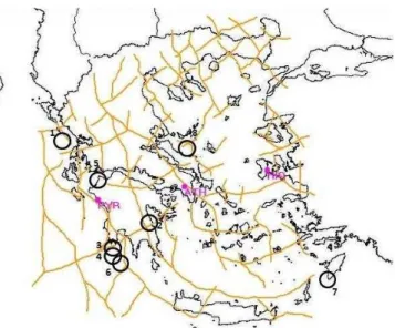
Geoelectric field data used in this work were collected from the database of the earth’s electric field (Thanassoulas, 2007). The implementation of these data to predict EQs has been widely used in Greece. There are three monitoring site that are installed in various areas of Greece; these are Athens (ATH), Pyrgos (PYR), and HIO (Hios).
monitoring
PYR (A),
PYR (A),
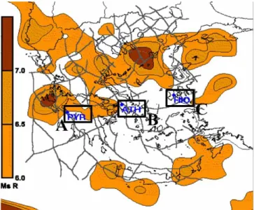
Fig. 1.Location of the monitoring sites PYR(A), ATH(B), and
HIO(C)(Thanassoulas, 2007).
Based on the measurements of the earth’s ground surface electric field, it is assumed that thex andy components of the electric field, i.e.ExandEy, are registered by horizontal dipoles. Thezcomponent, which is in the vertical direction, contains the same quality of information as thexandy com-ponents. However, due to technical difficulties, the measure-ment of the z component requires a vertical dipole with 150– 200 m depth in the ground. Because of this, thezcomponent has been ignored (C. Thanassoulas, personal communication, 2012). The total magnitude of the electric field measurement is given by
|E| =
q E2
x+E2y. (1)
2.1 Data collection
The database consists of valuable data from three dif-ferent monitoring sites in Greece; it is available at www.earthquakeprediction.gr (Thanassoulas, 2007). Mea-surements for this database consist of data which include 1440 data samples per day. The following monitoring sites in Greece are shown in Fig. 1:
– Athens (ATH) monitoring site, installed on 23 May 2003, operating presently.
– Pyrgos (PYR) monitoring site, installed on 15 April 2003, operating presently.
– Hios (HIO) monitoring site, installed on 18 March 2006, operated up to 2010.
Start
Read Geoelectric field
1st diff. of GFdiff
Peak detection algorithm
STFT method (Feature Extract)
Classification of earthquake-prone area and threshold determination
End
No
Yes Is 1st sig. Gfdiff
obtained in all monitoring sites?
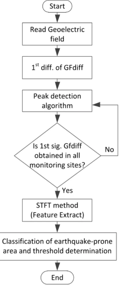
Fig. 2.Flowchart of the proposed feature extraction technique.
– PYR monitoring site to ATH monitoring site – 216.6 km.
– ATH monitoring site to HIO monitoring site – 209.5 km. – PYR monitoring site to HIO monitoring site – 425.6 km.
3 Proposed feature extraction technique
The proposed feature extraction technique in this work is based on the geoelectric field signal. The objective of this work is to analyse the characteristics of the signal which can be used as feature input to the EQ prediction system. Figure 2 shows the flowchart of the proposed technique. As shown in the flowchart, the raw data must be read properly. The dif-ferencing technique is then applied to the amplitude of the signal. This step is performed to observe the change in the signal prior to an EQ. Furthermore, the peak detection tech-nique is used to find the 1st significant change in the sig-nal. The short-time Fourier transform (STFT) technique is applied to investigate the characteristics of the spectrum of the 1st significant change in the geoelectric field. The classi-fication of an EQ-prone area, based on the location and the
(a)
(b)
Fig. 3.Raw geoelectric field data:(a)E–W and(b)N–S polarity
prior to 6.6R EQ on 6 January 2008.
Start
Calculate GFdiff
st
st
obtained?
monitoring site
End
Fig. 4.GFdiff prior to 6.6R EQ on 6 January 2008.
observation of the threshold value in the area, is made by this technique.
3.1 Reading of geoelectric field data
This stage involves the process of reading and inter-preting data extracted from the geoelectric field database (Thanassoulas, 2007). The raw data of the geoelectric field signal consists of two pairs of polarities, i.e. the E–W and N–S polarities. These two pairs of polarities need to be com-bined. The dataset consists of data from 3 different mon-itoring sites. Each dataset consists of 1440 samples with 5 columns, which can be described as follows:
– 1st column: time in hh:mm format
– 2nd column: the Gfdiff closest to E–W direction chan-nel 1 (E–W)
– 3rd column: ignored
– 4th column: the Gfdiff closest to N–S direction channel 3 (N–S)
– 5th column: ignored.
Start
Read Geoelectric field
Calculate GFdiff
Find max peak of segmented GFdiff
Is 1st sig. Gfdiff obtained?
Obtain the max peak of Gfdiff on
monitoring site
End
No
Yes
Detect 1st monitoring site that has max. peak of segmented Gfdiff/
7days
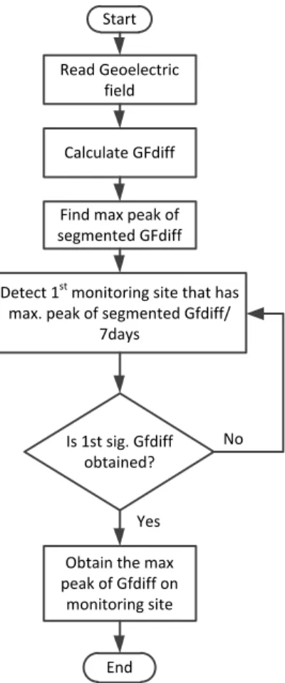
Fig. 5.Flow chart for algorithm of the determination of the 1st
sig-nificant change in geoelectric field prior to an EQ.
1, which provides the E–W polarity. The 4th column regis-ters the data from N–S polarity. The 3rd and 5th columns are the output of an analogue band-pass filter. These data consist of information from electric field measurements which have proven to have little change (C. Thanassoulas, personal com-munication, 2012). The total amplitude of geoelectric field can be found by using the following expression:
|E| =
q
EEW2 +E2NS. (2)
An example of the data from two polarities E–W and N–S are plotted in Fig. 3. The 1st row (a) contains data from E–W polarity. The second row (b) contains data from N–S polarity. This sample of data was taken on 9 December 2007 prior to the 6.6R EQ on 6 January 2008.
3.2 1st difference in the geoelectric field (GFdiff) signal
The purpose of implementing the 1st difference method for the signal is to observe the change in the signal over a certain period of time.E[n] denotes the value of the amplitude of Gfdiff at discrete time [n], and E [n−1] at discrete time [n−1]. The 1st difference of signal, also called geoelectric
Fig. 6.Example of STFT with adaptive sliding window.
field signal different, is given by
1E=E[n]−E[n−1], (3)
where1Eis the resulting GFdiff. An example of the GFdiff is shown in Fig. 4.
3.3 Peak detection algorithm
The idea behind the peak detection algorithm is to find the 1st maximum amplitude of GFdiff prior to an EQ. This 1st maximum amplitude of GFdiff is called the signal’s peak. The time when the peak of GFdiff occurs is referred to as the peak time. As illustrated in Fig. 4, the 1st significant change in Gfdiff with the amplitude of 493.5 [mV min−1] is found at the peak time of 260 min. If there is more than one peak with the same amplitude, the highest peak found would be selected. The algorithm for the peak detection of GFdiff is shown in Fig. 5. The maximum amplitude is detected by menting GFdiff by day. The maximum amplitude of the seg-mented signal is compared with those of others within 1 week of segmented signals. The maximum amplitude among the segmented signals is assigned as the 1st significant change in GFdiff. Once the 1st significant change in the Gfdiff is detected in one of the monitoring sites, the same procedure would be applied to the rest data from other monitoring sites. This procedure begins at the point where the 1st significant change from the previous monitoring sites is detected. 3.4 Adaptive short-time Fourier transform (STFT)
Start
Feature extraction
of GFdiff
Classification of
earthquake-prone
area
Threshold determination
based on location
Have all the
monitoring sites
obtained the
threshold?
Threshold obtained
for determination of
earthquake-prone
area
End
No
Yes
Fig. 7.Classification of EQ-prone area and threshold determination.
amplitude in the segmented data become the centre of the window to ensure that the important information is included in the window. This type of windowing technique is called an adaptive sliding window (shown in Fig. 6). Finally, the FFT technique is then applied to the windowed data.
In order to determine the best length of the segment and the most suitable window type, an experiment is performed on the GFdiff signal recorded at three different monitoring sites. The selection of the segment length and window function is performed to achieve the highest accuracy. In this work, the measurement accuracy refers to the condition where the geo-electric field data segment containing the peak time coincides with the spectral segment containing the maximum spectral amplitude. In the attempt to get the best length of segment that gives the best accuracy, 6 different segment lengths are used and compared. The segment lengths are 180 (which is equal to a sampling period of 3 h and dividing the data into
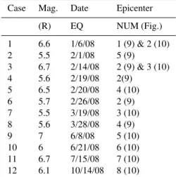
Table 1.List of EQs registered in Greece in 2008.
Case Mag. Date Epicenter (R) EQ NUM (Fig.) 1 6.6 1/6/08 1 (9) & 2 (10) 2 5.5 2/1/08 5 (9) 3 6.7 2/14/08 2 (9) & 3 (10) 4 5.6 2/19/08 2(9)
5 6.5 2/20/08 4 (10) 6 5.7 2/26/08 2 (9) 7 5.5 3/19/08 3 (10) 8 5.6 3/28/08 4 (9) 9 7 6/8/08 5 (10) 10 6 6/21/08 6 (10) 11 6.7 7/15/08 7 (10) 12 6.1 10/14/08 8 (10)
Fig. 8.EQs that occurred in Greece from January to October 2008
with magnitudes greater thanMs=6R (Thanassoulas et al., 2009).
Fig. 9.EQs that occurred in Greece from January to April 2008 with magnitudes greater thanMs=5R (Thanassoulas et al., 2008).
monitoring sites since it has high accuracy in detecting the highest amplitude based on the 1st significant difference in GFdiff.
3.5 Classification of EQ-prone area and threshold determination.
The 12 EQ datasets registered in Greece between 1 Jan-uary 2008 and 30 June 2008 have been classified based on the area where the EQs have happened. The frequency spec-trums of each are observed. The observation will determine the characteristics of the frequency spectrum for the GFdiff of that area and the threshold for GFdiff in each of the areas, as shown in Fig. 7.
4 Experimental result and discussion
The detailed analysis is performed on EQ data registered in Greece between 1 January 2008 and 30 June 2008. During this period 12 EQs took place. Of these 12, 5 EQs with mag-nitudes greater thanMs=5R (5R) and 7 EQs with magni-tudes greater thanMs=6R (6R), as shown in Table 1. The locations of these EQs and the corresponding magnitudes are shown in the maps in Figs. 8 and 9.
The 1st significant GFdiff prior to the EQs registered at the three monitoring sites has been investigated. For the analysis the GFdiff data is segmented and windowed. STFT is then applied to the windowed GFdiff. The analysis is then per-formed on the data before, on the day when the significant GFdiff is registered, and on the day which the EQ occurs. Table 2 shows the dates on which the analysis is performed.
As a matter of comparison, the data from the days of the normal condition, i.e. a few days before the 1st significant
0 1 2 3 4 5
1 3 5 7 9 11 13
Am
p.
Sp
ec
trum
PYR Monitoring Site:three different conditions of GFdiff (normal, first significant
different, day of EQ)-amp. spectrum vs. number of segments
Amp. freq of normal condition
Amp. freq of 1 SESD
Amp. freq of EQ
Fig. 10.Graphic of PYR monitoring site for three different
condi-tions of GFdiff.
0 0,5 1 1,5 2
1 3 5 7 9 11 13
Am
p.
Sp
ec
trum
ATH Monitoring Site:three different conditions of GFdiff (normal, first significant different,
day of EQ)-amp. spectrum vs. number of segments
Amp. freq of normal condition
Amp. freq of 1 SESD
Amp. freq of EQ
Fig. 11.Graphic of ATH monitoring site for three different
condi-tions of GFdiff.
difference in GFdiff, are also included in Table 2. Table 2 also includes the data from the day of the EQ and the 1st sig-nificant difference in GFdiff. The amplitudes of the spectrum of each day in the categories is compared. The result shows that the 1st significant differences of GFdiff have the most significant amplitude compared to that of the normal days and the day of EQ. Figures 10, 11, and 12 show that the 1st significant difference in GFdiff has the significant amplitude frequency compared to the other two.
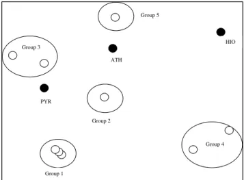
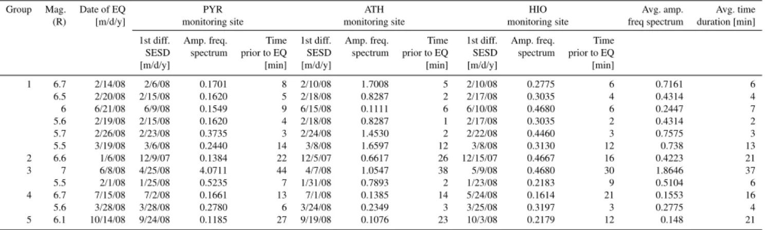
Grouping is performed in EQ prone areas from the 12 EQs which happened during the period of 1 January 2008 and 30 June 2008 – shown in Fig. 13. The classification of data based on the location is shown in Table 3. From the results the following can be shown:
Table 2.List of EQs registered in Greece in 2008.
Case Mag. Date of EQ PYR ATH HIO
[m/d/y] monitoring site monitoring site monitoring site 1st sig. Day of Day of 1st sig. Day of Day of 1st sig. Day of Day of
diff normal EQ diff normal EQ diff normal EQ condition condition condition
[m/d/y] [m/d/y] [m/d/y] [m/d/y] [m/d/y] [m/d/y] [m/d/y] [m/d/y] [m/d/y]
1 6.6 1/6/08 12/9/07 12/7/07 1/6/08 12/5/07 12/2/07 1/6/08 12/15/07 12/16/07 1/6/08 2 5.5 2/1/08 1/25/08 1/16/08 2/1/08 1/31/08 1/25/08 2/1/08 1/23/08 1/17/08 2/1/08 3 6.7 2/14/08 2/6/08 2/4/08 2/14/08 2/10/08 2/5/08 2/14/08 2/10/08 2/9/08 2/14/08 4 5.6 2/19/08 2/15/08 2/13/08 2/19/08 2/18/08 2/16/08 2/19/08 2/17/08 2/16/08 2/19/08 5 6.5 2/20/08 2/15/08 2/13/08 2/20/08 2/18/08 2/16/08 2/20/08 2/17/08 2/16/08 2/20/08 6 5.7 2/26/08 2/23/08 2/21/08 2/26/08 2/24/08 2/21/08 2/26/08 2/22/08 2/21/08 2/26/08 7 5.5 3/19/08 3/6/08 3/1/08 3/19/08 3/8/08 3/2/08 3/19/08 3/8/08 3/5/08 3/19/08 8 5.6 3/28/08 3/22/08 3/21/08 3/28/08 3/25/08 3/22/08 3/28/08 3/25/08 3/23/08 3/28/08 9 7 6/8/08 4/25/08 4/17/08 6/8/08 4/7/08 4/2/08 6/8/08 5/9/08 4/4/08 6/8/08 10 6 6/21/08 6/12/08 6/9/08 6/21/08 6/15/08 6/12/08 6/21/08 6/10/08 6/9/08 6/21/08 11 6.7 7/15/08 7/2/08 7/1/08 7/15/08 7/1/08 6/30/08 7/15/08 6/24/08 6/23/08 7/15/08 12 6.1 10/14/08 9/26/08 9/24/08 10/14/08 9/21/08 9/19/08 10/14/08 10/3/08 9/29/08 10/14/08
0 0,1 0,2 0,3 0,4 0,5
1 3 5 7 9 11 13
Am
p.
Sp
ec
trum
HIO Monitoring Site:three different conditions of GFdiff (normal, first significant different, day of EQ)-amp.
spectrum vs. number of segments
Amp. freq of normal condition Amp. freq of 1 SESD
Fig. 12.Graphic of HIO monitoring site for three different
condi-tions of GFdiff.
– The smaller the magnitude of the EQ, the shorter the time before the 1st significant GFdiff is detected prior to the EQ.
– The greater the magnitude of the EQ, the smaller the amplitude spectrum of GFdiff detected.
– The smaller the magnitude of the EQ, the greater the amplitude spectrum of GFdiff detected.
Therefore, it is highly probable that these unique charac-teristic of the 1st significant difference of GFdiff could be used as one of the characteristics in predicting and determin-ing the location and magnitude of EQs. This characteristic can be used as input to the identification system to predict any incoming EQs.
PYR
ATH
HIO
Group 4
Group 1 Group 3
Group 2
Group 5
Fig. 13.Grouping based on the area of 12 EQs in the period of
1 January to 30 June 2008.
5 Conclusions
Table 3.The classification of data based on the location.
Group Mag. Date of EQ PYR ATH HIO Avg. amp. Avg. time
(R) [m/d/y] monitoring site monitoring site monitoring site freq spectrum duration [min]
1st diff. Amp. freq. Time 1st diff. Amp. freq. Time 1st diff. Amp. freq. Time
SESD spectrum prior to EQ SESD spectrum prior to EQ SESD spectrum prior to EQ
[m/d/y] [min] [m/d/y] [min] [m/d/y] [min]
1 6.7 2/14/08 2/6/08 0.1701 8 2/10/08 1.7008 5 2/10/08 0.2775 6 0.7161 6
6.5 2/20/08 2/15/08 0.1620 5 2/18/08 0.8287 2 2/17/08 0.3035 4 0.4314 4
6 6/21/08 6/9/08 0.1549 9 6/15/08 0.1111 6 6/10/08 0.4680 6 0.2447 7
5.6 2/19/08 2/15/08 0.1620 4 2/18/08 0.8287 1 2/17/08 0.3035 2 0.4314 2
5.7 2/26/08 2/23/08 0.3735 3 2/24/08 1.4530 2 2/22/08 0.4460 3 0.7575 3
5.5 3/19/08 3/6/08 0.2440 14 3/8/08 1.6597 12 3/8/08 0.3130 12 0.738 13
2 6.6 1/6/08 12/9/07 0.1384 22 12/5/07 0.6617 26 12/15/07 0.4667 16 0.4223 21
3 7 6/8/08 4/25/08 4.0711 44 4/7/08 1.0547 38 5/9/08 0.4680 30 1.8646 37
5.5 2/1/08 1/25/08 0.5235 7 1/31/08 0.7893 2 1/23/08 0.2183 9 0.5104 6
4 6.7 7/15/08 7/2/08 0.1661 13 7/1/08 0.1385 14 5/24/08 0.1614 21 0.1553 16
5.6 3/28/08 3/28/08 0.2780 6 3/24/08 0.2349 3 3/25/08 0.3197 3 0.2775 4
5 6.1 10/14/08 9/24/08 0.1185 27 9/19/08 0.1076 23 10/3/08 0.2179 12 0.148 21
showing significant changes prior to the EQ. The results indi-cate that the 1st significant change in GFdiff prior to the EQ has the most significant amplitude of the spectrum compared to the day of normal conditions and the day on which the EQ occurs. Furthermore, it is found that this spectral amplitude is closely related to the magnitude, time, and location of the EQ that will occur. The greater the magnitude of the EQ, the longer the time before the 1st significant GFdiff prior to the EQ is detected. Likewise, the smaller the magnitude of the EQ, the shorter the time before the 1st significant GFdiff prior to the EQ is detected. The closer the distance between the location of the group and the monitoring site, the higher the amplitude of the spectrum of GFdiff that is detected. It is highly probable that these characteristics can be used as input parameters to the prediction system of the incoming EQ.
Acknowledgements. We thank Constantine Thanassoulas for his valuable advice, information, encouragement, and discussion in support of this work.
Edited by: F. Guzzetti
Reviewed by: two anonymous referees
References
Bhargava, N., Katiyar, V., K., Sharma, M., L., and Pradhan, P.: Earthquakes Prediction through Animal Behavior: A Review, In-dian J. Biomech., Special Issue, 159–165, 2009.
Dactron: Understanding FFT windows, Application Note, ANO14, 2003.
Gavinfarreli: Earthquake and Tsunami in Japan: The number of deaths and missing victims more than 18000, available at http: //www.worldnewco.com/4617, last access: November 2011.
Haryadi, M. : Earthquake and Tsunami kill more than 400 people in Aceh and North Sumatra, available at: http://www.asianews.it, last access: 15 March 2004.
Ikeya, M.: Earthquake and Animal: from Folk Legend to Science, World Scientific, 2004.
Japan Meteorological Agency: Earthquake information, available at: http://www.jma.go.jp/en/quake/, last access: 29 March 2011. Lazarus, D.: Physical Mechanisms for Generation and Propagation
of SESs. A critical review of VAN: Earthquake Prediction From Seismic Electric Signals, edited by: Lighthill, S. J., University College London, World Scientific Publishing, 1995.
Thanassoulas, C.: Short-term Earthquake Prediction, H. Dounias & Co., ISBN No:978-960-930268-5, 2007.
Thanassoulas, C.: “Short-term prediction” of large EQs by the use of “large scale piezoelectricity” generated by the focal area loaded with excess stress load, arXiv:0806.0360. v1, 2008. Thanassoulas, C. and Klentos, V.: How “Short” a “Short-term
pre-diction” can be? A review of the case of Skyros Island, Greece, EQ (26/7/2001,Ms=6.1). Geophysics, arXiv:1002.2162, 2010.
Thanassoulas, C. and Tselentis, G.: Periodic variations in the Earth’s electric field as earthquake precursors: results from recent experiments in Greece, Tectonophysics, 224, 103–111, 1993. Thanassoulas, C., Klentos, V., and Verveniotis, G.: Extracting
preseismic electric signals from noisy Earth’s electric field data recordings, The “noise injection” method, Geophysic, Arxiv:0807.4298/2008, 2008.
USGS: Magnitude 9.0-Near the East Coast of Honshu, Japan 2011 March 11 05:46:23 UTC, available at http://earthquake.usgs.gov/ earthquake/eqinthenews/2011, last access: April 2011.