Mechanistic Mathematical Modeling Tests
Hypotheses of the Neurovascular Coupling in
fMRI
Karin Lundengård1,2, Gunnar Cedersund3,4, Sebastian Sten1, Felix Leong1,
Alexander Smedberg1, Fredrik Elinder4, Maria Engström1,2*
1Department of Medical and Health Sciences, Linköping University, Linköping, Sweden,2Center for Medical Image Science and Visualization (CMIV), Linköping University, Linköping, Sweden,3Department of Biomedical Engineering, Linköping University, Linköping, Sweden,4Department of Clinical and
Experimental Medicine, Linköping University, Linköping, Sweden
Abstract
Functional magnetic resonance imaging (fMRI) measures brain activity by detecting the blood-oxygen-level dependent (BOLD) response to neural activity. The BOLD response depends on the neurovascular coupling, which connects cerebral blood flow, cerebral blood volume, and deoxyhemoglobin level to neuronal activity. The exact mechanisms behind this neurovascular coupling are not yet fully investigated. There are at least three different ways in which these mechanisms are being discussed. Firstly, mathematical models involv-ing the so-called Balloon model describes the relation between oxygen metabolism, cere-bral blood volume, and cerecere-bral blood flow. However, the Balloon model does not describe cellular and biochemical mechanisms. Secondly, the metabolic feedback hypothesis, which is based on experimental findings on metabolism associated with brain activation, and thirdly, the neurotransmitter feed-forward hypothesis which describes intracellular pathways leading to vasoactive substance release. Both the metabolic feedback and the neurotrans-mitter feed-forward hypotheses have been extensively studied, but only experimentally. These two hypotheses have never been implemented as mathematical models. Here we investigate these two hypotheses by mechanistic mathematical modeling using a systems biology approach; these methods have been used in biological research for many years but never been applied to the BOLD response in fMRI. In the current work, model structures describing the metabolic feedback and the neurotransmitter feed-forward hypotheses were applied to measured BOLD responses in the visual cortex of 12 healthy volunteers. Evaluat-ing each hypothesis separately shows that neither hypothesis alone can describe the data in a biologically plausible way. However, by adding metabolism to the neurotransmitter feed-forward model structure, we obtained a new model structure which is able to fit the esti-mation data and successfully predict new, independent validation data. These results open the door to a new type of fMRI analysis that more accurately reflects the true neuronal activity.
a11111
OPEN ACCESS
Citation:Lundengård K, Cedersund G, Sten S, Leong F, Smedberg A, Elinder F, et al. (2016) Mechanistic Mathematical Modeling Tests Hypotheses of the Neurovascular Coupling in fMRI. PLoS Comput Biol 12(6): e1004971. doi:10.1371/ journal.pcbi.1004971
Editor:Jörn Diedrichsen, University College London, UNITED KINGDOM
Received:October 23, 2015
Accepted:May 4, 2016
Published:June 16, 2016
Copyright:© 2016 Lundengård et al. This is an open access article distributed under the terms of the Creative Commons Attribution License, which permits unrestricted use, distribution, and reproduction in any medium, provided the original author and source are credited.
Data Availability Statement:All relevant data are within the paper and its Supporting Information files.
Author Summary
Functional magnetic resonance imaging (fMRI) is a widely used technique for measuring brain activity. However, the signal registered by fMRI is not a direct measurement of the neuronal activity in the brain, but it is influenced by the interplay between the metabolism, blood flow and blood volume in the active area. This signal is called the blood-oxygen-level dependent (BOLD) response and occurs when the blood supply to the active area increases in response to neuronal activity. The mechanisms that the cells use to influence the blood supply are not fully known, and therefore it is difficult to know the true neuronal signalling only from inspection of the fMRI signal. In this article, we present a new mathe-matical model built on the physiological mechanisms thought to underlie the BOLD response. We could successfully fit the model to data and predict the activity caused by new stimuli. By using the validated model we investigated physiological mechanisms that cause different parts of the BOLD response.
Introduction
Functional magnetic resonance imaging (fMRI) measures brain activity by detecting associated changes in blood oxygenation through the blood-oxygen-level dependent (BOLD) response. The BOLD response is caused by time-dependent changes in deoxyhemoglobin (dHb) concen-tration [1]. Although the BOLD response reflects neuronal activity through the neurovascular coupling [2], the mechanisms causing the response are still not fully understood. Here, we investigate these mechanisms by mathematical modeling using a systems biology approach.
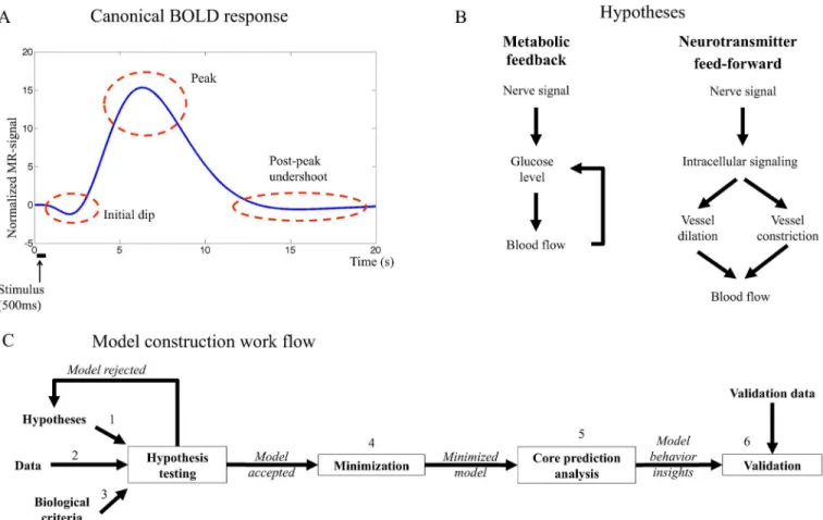
The BOLD response endures approximately 15 seconds after a short neural stimulus and it has several characteristic features (Fig 1A) [3]: (i) During the first couple of seconds a shallow undershoot, referred to as the initial dip, is sometimes observed in activated areas of the brain [4][5]. The initial dip is hypothesized to reflect an increased cerebral metabolic rate of oxygen (CMRO2) that is followed by an increase of dHb content in the blood. (ii) At 6–8 s after the
stimulus, the BOLD response peaks as a result of increased cerebral blood volume (CBV) and/ or increased cerebral blood flow (CBF). (iii) After the peak, the BOLD response decays and shows a post-peak undershoot before returning to baseline. The mechanisms controlling these processes (i-iii) remain unresolved, and there are at least three different approaches to under-stand these mechanisms.
The first approach is centered around mathematical modeling. One of the most common approaches is to model the hemodynamic response function (HRF) using the so-called Balloon model [6][7][8][9], which has been of paramount importance in the development of fMRI image analysis [10]. The Balloon models describe the interplay between CMRO2, CBV, and
CBF. The dynamics of these three entities are described in part by purely phenomenological descriptions, such as convolutions with the covariate gamma functions, and in part by physical modelse.g.describing the dynamics between CBV and CBF in an expanding balloon. In other words, these Balloon models typically do not incorporate intracellular and biochemical mecha-nisms involved in cell metabolism or intra-cellular signaling processes related to the BOLD response. Nevertheless, there do exist mathematical models that also incorporate intracellular metabolism [11], but ultimately even these models explain the actual BOLD response via the Balloon model, which appears as a sub-model in the complete model. Other models, which are not extensions of the Balloon model, describee.g.spatiotemporal properties of the BOLD response as hemodynamic traveling waves [12] or oxygen transport in the brain by modeling CBF with a linear flow model and CMRO2using a gamma function [13].
The second approach to understanding the BOLD response is centered around the so-called metabolic feedback hypothesis. According to this classical hypothesis (Fig 1B, left), the BOLD response is the result of a tight connection between glucose metabolism and blood flow; when the brain is activated, the neurons consume more energy, resulting in decreased blood glucose and oxygen levels [14][15], which trigger a feedback signal increasing CBF to meet metabolic demands. In other words, the metabolic hypothesis is centered around a feedback control to keep glucose level constant.
The third and final approach relevant to this paper is referred to as the neurotransmitter feed-forward hypothesis. This hypothesis is reviewed ine.g[16], and it is today more actively discussed than the metabolic feedback hypothesis. The neurotransmitter feed-forward hypoth-esis (Fig 1B, right) suggests sequential feed-forward signaling where neurotransmitters,
Fig 1. A. Canonical BOLD response to a brief stimulus. The initial dip, the peak and the post-peak undershoot are marked in the figure.B. Main mechanisms of the hypotheses investigated in this work.The metabolic hypothesis (left) suggests feedback signaling where decreased blood glucose levels trigger cerebral blood flow (CBF) increase, which in turn delivers more glucose to the activated area. The neurotransmitter feed-forward hypothesis (right) suggests feed-feed-forward signaling with two competing arms where the negative arm results in decreased CBF and the positive in increased CBF. The balance between the actions in both arms determines the shape of the BOLD response.C. The model construction workflow in this article.The biological hypothesis is translated to equations firmly based in the biological mechanisms (1), this system of equations is the model structure. Data is collected (2) and the model structure is fitted to the data by optimizing the parameters. If the model can not fit the data, the model structure is rejected or altered. If the model can fit the data, it is analyzed and evaluated to control that it does so in a biologically plausible way (3). If the model does not fulfil these criteria, it is rejected. If the model is accepted, the model is minimized in order to identify key mechanisms of the system (4) and core predictions of not yet performed experiments are made (5). In the next step, new data are collected, using experimental setup based on previous predictions, and the model predictions are compared to the new data set (6). If the predictions are satisfactory, the model is accepted. If the predictions fail the model is rejected, and a new iteration of alterations and analyses is performed taking both old and new data into consideration. The model construction workflow can be iterated as many times as needed until a satisfactory model has been reached.
especially glutamate, cause neurons and astrocytes to activate a chain of intracellular events, involving the release of nitric oxide (NO) or arachidonic acid (AA) metabolites, which in turn control constriction and dilation of the blood vessels. In this way, the feed-forward system
“anticipates”the increased need, and goes directly from increased neural activity to increased blood supply.
Of the three approaches mentioned above, only the first involves mathematical modeling and these models are focused mainly on the phenomenological description of the HRF. How-ever, although the metabolic feedback and the neurotransmitter feed-forward hypotheses have been extensively studied through purely experimental approaches, these two hypotheses have never been implemented as mathematical models. It is therefore not known whether the pro-posed mechanisms of the metabolic feedback and the neurotransmitter feed-forward hypothe-ses actually would produce a BOLD response or not.
Model-based testing of mechanistic hypotheses has been done in biological research for many years, and has gained increased interest through the rise of systems biology. As men-tioned above, mathematical models are already standard when analyzing fMRI, but these mod-els are partially phenomenological and have not been developed to test intracellularly centered hypotheses such as the metabolic feedback and the neurotransmitter feed-forward hypotheses. In contrast, intracellular mechanistic models are the main focus in systems biology, and here hypotheses are formulated as direct representations of the assumed biochemical reactions [17] [18]. This formulation allows for a new type of data analysis, which revolves around two steps: (i) rejections and (ii) uniquely identified core predictions (Fig 1C). This model-based approach provides a more comprehensive, correct, and verifiable analysis, compared to analyses based on inspection and reasoning. In other words, while it sometimes may seem logical to draw a certain conclusion based on visual inspection of some given data, we and others have repeat-edly shown that such manual inspections often lead to incorrect, or at the very least incomplete, interpretations of the data [19,20].
In this paper, we provide a first systems biology analysis of the metabolic feedback and the neurotransmitter feed-forward hypotheses (Fig 1B) with regards to their ability to describe the BOLD response. We show that neither of the two hypotheses alone can satisfactorily describe the response. In contrast, a feed-forward mechanism with added oxygen metabolism can pro-vide a satisfactory explanation of the BOLD response measured in fMRI.
Materials and Methods
Mechanistic modeling
Mechanistic modeling has within systems biology evolved into an iterative process, which alter-nates between model-based data analysis and the collection of new experimental data. This pro-cess is outlined inFig 1C. In Step 1, existing hypotheses are reformulated into a set of
identify key mechanisms of the system and facilitate computation and overview of the model. In Step 5, further analysis of the explanations consists of the identification of relevantcore pre-dictions, i.e. uniquely identified predictions with uncertainty [21]. These predictions may some-times be suitable for experimental testing, and this leads to collection of new data, Step 6, which in turn leads to the final testing and analysis of the model. Sometimes, interesting model behav-iors are discovered in this final step, which might lead back to the hypothesis testing step for further investigation. In this way, systems biology modeling has the potential to be a never-end-ing cycle, but for each step that is passed, new information about the system is obtained. The iterations end when the model is satisfyingly detailed or no more suitable data can be gathered.
Model structures are formulated as ordinary differential equations. The models herein are formulated using ordinary differential equations (ODEs), which have the following general structure
_
x¼fðx;px;uÞ ð1Þ
xð0Þ ¼x
0 ð2Þ
by¼gðx;px;py;uÞ ð3Þ
wherexare the states, describing the concentration or amount of various substances; wherex_
represents the derivative of the states with respect to time; wherefandgare non-linear smooth functions; wherepxare the parameters used to calculatef, here kinetic rate constants; whereu
is the input, here the visual stimuli given to the subjects; wherex(0) contains the values of the states at timet= 0, and where these values are described by the parametersx0; wherebyare the
simulated model outputs corresponding to the measured experimental signals, here the BOLD response; and wherepyare parameters only appearing in the measurement equations, here
scaling parameters. Recall that there are three types of parameters,p, with potentially unknown values,
p¼ ðpx;x0;pyÞ ð4Þ
How these parameters are determined and evaluated is described below. Note thatx,u, andy
depend ont, but that the notation is dropped unless the time-dependence needs to be especially stated, as inEq (2). All symbols in Eqs (1), (2) and (3) are vectors.
In the formulation of mechanistic hypotheses into ODEs, there are three levels, which are distinguished using the following notation. Thehypothesis xis denotedMx, wherexhere has
the valuesm,n, andnm, corresponding to the metabolic feedback, the neurotransmitter feed-forward, and the extended neurotransmitter feed-forward hypothesis hypotheses, respectively. Each of these hypotheses have been implemented using alternative sets of equations, corre-sponding to further specifications and assumptions, and these alternatives are tagged using additional numbers. Such a set of equations is usually referred to as amodel structure[22]. Finally, a model structure is referred to as amodelif a set of specific parameter values has been chosen, and these parameters are specified with a final bracket. For example,Mn4ðbp4Þdenotes
the 4th model structure implementing the neurotransmitter feed-forward hypothesis, which should be analyzed using the parameters inbp4.
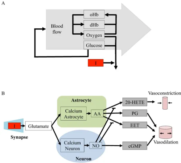
Model structures. The metabolic model is centered around a feedback control loop, where the rate of blood flow is altered to keep the blood glucose or oxygen levels constant. A sche-matic overview of this model is shown inFig 2A. A specific implementation of this hypothesis,
Mm3, is plotted in Fig B inS1 Appendix. Fig B inS1 Appendixis aninteraction graph, which
ine.g.[23][24]. More specifically, this means that the non-regulated rates are given by mass-action kinetics, and each differential equation is given by the sum of the in- and out-going reac-tions, weighted by the stoichiometric matrix. There are three exceptions to this interpretation. First, the blood flow is a variable, not a state, and it affects all four states oxyhemoglobin (oHb), dHb, glucose, and molecular oxygen (O2) by transporting the species in and out of the studied
vessel. Second, the stoichiometries of the metabolism in the stimulated and the basal states are different and not specified in Fig B inS1 Appendix. Finally, the delay boxes means that inter-mediate states have been introduced fore.g.glucose and its influence on the blood flow. This means that the ODE fore.g.oHb is given by
d½oHb
dt ¼k1f½dHb½O2 k1b½oHb þvflow½oHbbasal vflow½oHb ð5Þ
Fig 2. Schematic overviews of the initial model structures evaluated in this paper.I = the stimulus, which is the input to the model.A. Schematic overview of the metabolic feedback model structure.oHb and dHb are oxyhemoglobin and deoxyhemoglobin, respectively.B. Schematic overview of the neurotransmitter feed-forward model structure.The neurotransmitter feed-forward hypothesis is described in more detail in [16]. Green
area = astrocyte, blue area = neuron, grey area = blood vessel. Calcium neuron and calcium astrocyte = calcium ion (Ca2+) level in the cell, NO = nitric oxide, cGMP = cyclic guanosine monophosphate, AA = arachidonic acid, EET = epoxyeicosatrienoic acids, PG = prostaglandins and 20—HETE = hydroxyeicosatetraeonic acid. Pointed arrows signify positive interactions and flat arrows signify inhibition. Specific implementations and interaction graphs are available inS1 Appendix.
wherek1fandk1bare reaction rate constants; wherevflowdenotes the bloodflow, and where
[oHb]basaldenotes the concentration of oHb in the bloodflowing in to the studied area. Similar
equations describe states and reactions seen inFig 2A. All equations and model parameters are specified in detail inS1 Appendix, where also all scripts used for the analyses in the paper can be found. The underlying assumptions of the model are discussed in Section“Assumptions and Limitations”.
The neurotransmitter hypothesis is centered around a feed-forward signaling system, where the regulation of the blood flow is given by the balance of positive and negative regulations. The first model structure corresponding to this hypothesis,Mn1, is depicted inFig 2B. The
ODEs are directly specified by the interaction graph in Fig C inS1 Appendix, using standard and already mentioned conventions. As can be seen in both figures, the input signal triggers release of glutamate into the synaptic cleft. Glutamate increase triggers calcium-permeable non-methyl D aspartate (NMDA) activated channels in neurons and astrocytes to open, letting calcium flow into the cells. In neurons, the calcium influx leads to an increase in the concentra-tion of nitric oxide (NO) that stimulates the producconcentra-tion of vasodilating cyclic guanosine mono-phosphate (cGMP). In the astrocyte, calcium ions increase the production of arachidonic acid (AA), whose metabolites epoxyeicosatrienoic acids (EET), prostaglandins (PG) and hydroxyei-cosatetraeonic acid (20-HETE) effect blood vessel radii. The interaction graph in Fig C inS1 Appendixis based on a similar figure in Attwellet al.[16].
Fitting to data. Once the model structure has been formulated (Fig 1C, Step 1 in the modeling workflow) and data has been collected (Step 2, data acquisition described below), the parameters,p, need to be determined. The parameter evaluations are centered on the following cost function
w2ðpÞ ¼
XN
i¼1
ðyðtiÞ byðtijpÞÞ 2
sðtiÞ
2 2w
2
ðdÞ þadditional terms ð6Þ
wherey(t) are the measured data points at timet; wherebyðpÞare the corresponding simulated data points at timet; whereNis the number of time-points; and whereσ(t) is the measurement
uncertainty at timet. The summation inEq (6)sums the squared and normalized residuals, indi-cating how far the simulationsbyare from the datay. The additional terms (also referred to as
“punishments”,“weights”or“penalties”) are included only when additional requirements are needed. Such requirement might be the presence of an initial dip in the BOLD response (as described in the evaluation criteria in Section“Model evaluation”). If the additional requirements are fulfilled, the additional terms equal zero. If the additional requirements are not fulfilled, the additional terms are increased to force the optimization away from such parameter sets.
In practice, the parameters are determined by optimizingχ2(p) overp, using the function
“simannealingSBAO”in the Systems Biology toolbox for Matlab [25]. In other words, the opti-mal parametersbpare given by
b
p¼ arg minw2ðpÞ ð7Þ
Model evaluation. The final part of the hypothesis testing in the model construction work flow is to check whether the obtained model fulfills the set criteria of the study. In this study the model structure must be able to:
The first criterion is tested using theχ2test. This test is based on the observation that the
cost function inEq (6)follows aχ2distribution if the measurement noise follows a normal
dis-tribution, with standard deviationσ. Therefore, the resulting cost is compared to the inverse of
a cumulativeχ2distribution, where the degrees of freedom are given by the number of data
points minus 1. In practice, one decides whether the cost is acceptable or not by comparing the cost with the cut-off value [18]. In our case this means that the cut-off have been 49.8 (χ2,α=
0.05, df = 35) for the estimation data. The second criterion is evaluated via simple simulations, and their fulfillment is ensured by adding these criteria as additional terms inEq (6).
It is necessary that the model output can fit the data (Criterion 1), but this criterion is not enough to test the underlying mechanism. Therefore, the second and third criteria are added. Most notably, the initial dip is often absent in collected data, although it has been proposed to carry important information about the underlying neuronal activity (discussed further in Dis-cussion: The Initial Dip). The second criterion ensures that the model has the mechanisms required to simulate an initial dip if it is fitted to a data set where it is expressed.
The third criterion is more vaguely phrased, as biological plausibility depends on the mech-anisms present in each specific model structure. The third criterion is therefore developed and tested separately for each model structure.
Model minimization and comparison. Mechanistic models describing biological systems often become complex with several interacting states and parameters. Such a model, although good for illustrating the biological hypothesis, is computationally heavy and poses difficulties during overview and analysis. A strategy to analyze how the model describes the main mecha-nisms behind the BOLD response is model minimization (Step 4 inFig 1C). Model minimiza-tion is done by excluding parts of the original model and optimizing it anew to the data. If the reduced model is still able to describe the data, yet another state or a group of states can be excluded. The minimal model has been reached when no more states or reactions can be excluded without the model loosing the ability to fit to the data.
Reducing the number of parameters in the model often makes it harder for the model to fit the data, and thereby the cost of the model will increase compared to the original version of the model. In order to see if the model fit is good enough to compensate for the increased cost, a likelihood ratio test can be performed. If
w2ðnm1 nm2Þ 2 ðVm1ðbpm1Þ Vm2ðbpm2ÞÞ ð8Þ
then the minimized model is not significantly worse at describing the data than the original model, despite its reduced number of parameters. The symbolnmiis the number of parameters
in the model structureiandVmiðbpmiÞis the lowest cost that the optimization has found for the
same model structure.
Core prediction analysis. The final model analysis is referred to as core prediction anal-ysis, seen in Step 5 inFig 1C. Core prediction analysis is making predictions with uncertain-ties [21] and [26], which are then tested towards validation data (Step 6 inFig 1C). More precisely, the predictions are analyzed for not only one, but for all parameter sets that pass a
χ2test and thereby can describe the estimation data. In practice, we do not analyze the
Experimental data
Subjects. Time series data of the BOLD response were collected from the visual cortex of 13 healthy subjects. The subjects were instructed not to consume caffeine, alcohol, or use nico-tine on the day of examination. All subjects gave their written informed consent and the study was approved by the Regional Ethical Review Board in Linköping (M74-06).
Individuals failing to fill the criteria set in the standard MR safety screening form were excluded from participating in the study. Maximum allowed translational head movement was limited by a cut-off value of 3.5 mm (the one-dimensional size of one voxel). After reviewing the head movement of each subject, one subject (out of 13) was excluded from further analysis. Thus, 12 subjects (mean age = 23.5 years SD: 4.4, range = 19–35 years) remained in the study. Seven subjects were men and five were women.
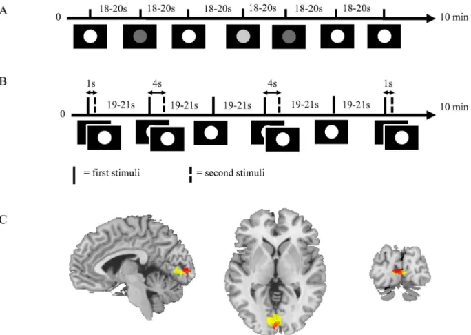
Visual stimulation. The study was designed in the form of two experiments, theintensity
and thefrequencyexperiment (Fig 3A and 3B, respectively). These experiments were based on brief visual stimulation using a sparse event-related design in order to isolate individual BOLD responses. The principal visual stimulus consisted of filled white or grey circles shown for 500
Fig 3. A. Intensity experimental paradigm.The figure shows the principal experimental design where the stimuli consisted of circles in white and two shades of grey on a black background. White circle stimulus was the primary stimulus and was used to generate the estimation data.B. Frequency experimental paradigm.The figure shows the principal experimental design where the stimuli consisted of white circles on black background. Sometimes a single stimulus was shown and sometimes paired stimuli were shown with inter-pair interval (IPI) of 1 s or 4 s.C. Group level activation in the visual cortex.The figure shows activation in the visual cortex during the intensity (red) and the frequency (yellow) experiments across the whole group of subjects. Only activation that passes p = 0.05, family wise error (FWE) corrected threshold is shown in the figure.
ms on a black background. Each stimulus was followed by a randomly jittered intertrial interval (ITI) to reduce adaptation effects. During the ITI a grey focus cross was presented against black background.
Nine subjects performed the intensity experiment first and the frequency experiment last. Four subjects performed the experiments in the opposite order. In both experiments the visual stimuli were presented using video goggles (VisuaStimDigital, Resonance Technology Inc., USA) with a built in screen and correction lenses. The experimental paradigm was presented using the software package SuperLab 4.5 (Cedrus Corporation, San Pedro, CA, USA) using a Windows XP computer. The presentation of the stimuli was randomized using SuperLab’s ran-domize function, randomizing once per group of participants. Thus, the stimulus onset times did not vary between individuals.
The intensity experiment and the frequency experiment had three stimuli each. In both experiments, the single, bright white circle shown for 500 ms, was used as primary stimulus. The time course of the primary stimulus of each experiment was used as estimation data when the models were fitted.
In the intensity experiment (Fig 3A), the color of the circle was white, light grey, or dark grey. Each stimulus was presented a total of 9 times each with an ITI of 18 to 20 seconds. Thus, the experiment contained 27 trials with a total runtime of approximately 10 minutes.
The frequency experiment (Fig 3B) included the bright white circle on black background presented in three different frequency modes. The first mode consisted of the primary stimulus, which was the same as in the intensity experiment. In the other modes, the stimuli were paired, with an inter-pair interval (IPI) of 1 or 4 seconds, respectively. Each stimulus was presented 8 times each with an ITI of 19 to 21 seconds. The experiment contained 24 trials with a total run-time of approximately 10 minutes.
MRI. All experiments were performed with a Philips Ingenia 3 T MR scanner and a 24-channel head coil. BOLD-images were acquired using a gradient echo sequence sensitive for the BOLD contrast using the following parameters: repetition time (TR) = 500 ms, echo time (TE) = 30 ms, resolution = 3.5 mm isotropic, field of view = 224 mm × 196 mm × 35 mm, flip angle = 60 degrees, echo planar imaging (EPI) factor = 29, sense factor = 2.2. Ten axial slices were collected, oriented from the calcarine sulcus to the cingulate gyrus. The number of acquired volumes (number of dynamics) was 1160 per experiment. T1-weighted (T1W) scans
were obtained for each individual, as a basis for co-registration of the BOLD-images to high-resolution anatomical images. The following parameters were used for T1W imaging: field of view = 240 mm × 240 mm × 180 mm, voxel size = 0.5 mm × 0.5mm × 0.6 mm, TR = 13 ms, and TE = 6.3 ms.
Image analysis. Images from each subject were preprocessed using SPM8 (www.fil.ion. ucl.ac.uk/spm). All images were re-aligned to the first image in the time series to correct for motion during scanning. Thereafter the images were co-registered to the T1W anatomical ref-erence and normalized to the standard template in MNI (Montreal Neurological Institute) space. The normalized images were smoothed with 7 mm Gaussian kernel to reduce noise and ameliorate inter-subject differences in brain anatomy during the voxel wise group analyses.
subtracting the signal value of the last time point before the stimulation from the values of the entire BOLD time series corresponding to each stimulus. BOLD responses from each stimulus were first averaged over each individual and thereafter over the group.
Results
Brain activation during visual stimulation
Visual stimulation during both the intensity and the frequency experiment elicited significant activation in bilateral primary visual cortex, p<0.05 family wise error (FWE) corrected for multiple comparisons (Fig 3C). FWE is a Bonferroni-correction applying the random-field the-ory (RFT) to control the FWE rate by assuming that the data follow certain specified spatial patterns [28]. The Montreal Neurological Institute (MNI) co-ordinates of the activation peaks were: [-2, -96, 4] and [-10, -84, 2] for the intensity and the frequency experiments, respectively.
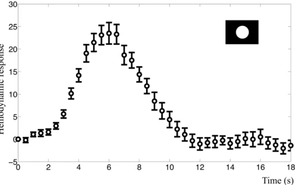
The mean BOLD response to the primary visual stimuli in both experiments had a charac-teristic response peak at approximately 6 s after the stimuli (Fig 4). Peak amplitude was 23.5 (2.12% signal change) in the intensity experiment and 19.8 (1.95% signal change) in the fre-quency experiment. We also observed a post-peak undershoot, but neither of the resulting BOLD responses in any subject displayed a clear initial dip.
Rejection of the metabolic feedback model structure
Blood flow needs to be controlled by glucose. When implementing the metabolic feed-back model initial attempts were made with a model structure,Mm1, where oxygen levels
con-trolled the blood flow, but such a model structure could neither fulfill the criteria of displaying a post-peak undershoot nor fit the data, as can be seen in Fig A inS1 Appendix. The model structure was therefore rejected at Steps 2 and 3 in the modeling workflow (Fig 1C). If glucose
Fig 4. BOLD response in the visual cortex.The figure shows the mean BOLD response and standard error for the primary visual stimulus of the intensity experiment. This time course was used as estimation data when the models were fitted. They-axis represents normalized MR signal in arbitrary units.
instead of oxygen was selected to control blood flow, it was possible to simulate the shape of the BOLD response by varying the degree of aerobicvs.anaerobic metabolism, as is done in model structureMm2.
Stimulated metabolism must be partly anaerobic to obtain both an initial dip and a peak. Further tests ofMm2in the hypothesis testing revealed an important insight regarding a
necessary difference between the basal metabolism and the stimulated metabolism. This differ-ence concerns the relationship between oxygen and glucose consumption. If the metabolism is continuously aerobic,i.e.if the ratio of oxygen and glucose consumption is equal during basal state and stimulation, the effect of increased metabolism is oxygen level reduction (Mm2ðbp1Þ,
Fig 5B,first three seconds). This oxygen reduction persists until the bloodflow is sufficiently up-regulated to normalize oxygen levels (at approximately 10 seconds,Fig 5B). In other words, in this situation, there is an initial dip but no peak.
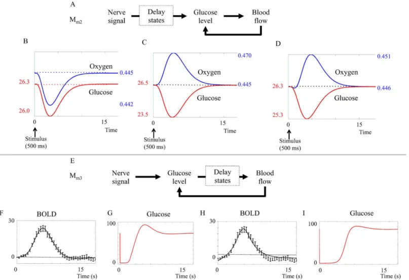
Fig 5. Results from the metabolic feedback model. A. Placement of the delay states (dashed squares) in modelMm2.The delay states are placed
mainly between the neuronal activity and the glucose metabolism.B-D. Impact of aerobic versus anaerobic metabolism.B. Predicted BOLD response of Mm2assuming (CMRO2/CMRglu)basal= (CMRO2/CMRglu)stimuli. C. Predicted BOLD response ofMm2assuming (CMRO2/CMRglu)basal>(CMRO2/
CMRglu)stimuli= 0. D. Predicted BOLD response ofMm2assuming (CMRO2/CMRglu)basal>(CMRO2/CMRglu)stimuli>0. To display both an initial dip and a
peak, the model must have a metabolism that is more anaerobic during stimulation, compared to the metabolism during the basal state.E. Placement of the delay states in modelMm3.The delay states are placed mainly between the glucose metabolism and the blood flow.F-G. The glucose response inMm3.
G and H. The best fit does pass a Chi-square goodness-of-fit test, but lacks an initial dip and glucose goes down to zero for several seconds. H-I.Mm3can be
forced to display an initial dip, but then it has no undershoot and glucose must still go down to almost zero in order for the feedback to kick in.
Conversely, if the stimulated metabolism is completely anaerobic,i.e.if glucose but not oxy-gen metabolism is increased during stimulation, the effect would be an increase in blood flow to compensate for decreased glucose levels. Oxygen levels will then increase as the increased blood flow brings more oxygen to the capillaries, but this extra oxygen is not metabolized. In this situa-tion (which can be seen inMm2ðbp2Þ, simulated inFig 5C) there is a peak but no initial dip.
A combination,Mm2ðbp3Þ, where the stimulated metabolism is adjusted to be more
anaero-bic than the basal metabolism, both an initial dip and a following peak is produced (Fig 5D). In practice, the proportion of aerobic and anaerobic metabolism was varied by changing the number of oxygen molecules used during glucose metabolism. The parameter sets where the proportion parameters are changed can be seen in section 1.2.3 inS1 Appendix. We did not
find any versions of the model that did not require a more anaerobic metabolism during stim-ulation, and we therefore conclude that, if the metabolic feedback hypothesis is true, the metabolism must be more anaerobic during stimulation compared to the metabolism during basal state.
The metabolic feedback model structuresMm2andMm3have problems with predicted glucose levels. The metabolic feedback model structureMm2assumes glucose regulation of
blood flow and a more anaerobic process during stimulation.Mm2has a statistically acceptable
fit to the intensity data primary stimulus according toχ2goodness-of-fit test (cost = 45.5,
cut-off = 49.8). However, as can be seen inFig 5D, the glucose state decreases very slowly. This means that glucose minimum occurs simultaneously with the BOLD response peak,i.e. simul-taneously with the oxygen peak. This behavior contradicts the basic principle of the metabolic hypothesis and is caused by delay states inserted between the neuronal signal and the glucose metabolism in the model structure (dashed square inFig 5A). These delay states between the stimulus and the glucose metabolism contribute to the shape of the initial dip, but have no bio-logical interpretation.
A new model structure,Mm3, was constructed. In the model structureMm3(Fig 5F), the
delay states are placed between the metabolism and the blood flow, and represent the action of smooth muscle controlling the radius of the blood vessels. The fit of (Mm3ðbp4Þ) and (Mm3ðbp5Þ)
is shown inFig 5F and 5G. As can be seen, the model structureMm3is incapable of displaying
both the initial dip and a post-peak undershoot simultaneously. Furthermore, bothfits ofMm3
entail problems with the predicted glucose levels. The graphs depicting glucose levels (Fig 5G and 5I) show that the glucose levels decrease to almost zero (<5% of the original value) within
thefirst 2 seconds after the stimulus, and in the case of an initial dip (Fig 5I), remain low until the peak of the BOLD response has passed. Even though the exact stimulated glucose dynamics is unknown, we consider this predicted behavior unrealistic.
The metabolic feedback hypothesisMmis rejected. In summary, the metabolic feedback
hypothesisMmcan describe the experimental data, but is still rejected during the hypothesis
testing for two reasons. Firstly, it cannot produce both an initial dip and a post-peak under-shoot in the same simulation. Secondly, and most importantly, the tested metabolic feedback model structures are not biologically plausible, because they predict depletion of glucose levels and unrealistically fast and/or slow time course of stimulated glucose dynamics.
Rejection of the neurotransmitter feed-forward model structure
Fitting of the neurotransmitter feed-forward model. The neurotransmitter feed-forward modelMn1ðbp6Þcanfit the estimation data from the primary stimulus. As can be seen inFig 6A,
no metabolism, and under this assumption, the bloodflow can be used as a direct proxy for the output, i.e. for the oxygen, dHb, and oHb levels as the output of the model structureMn1.
The main mechanism in the neurotransmitter feed-forward model is a balance between vasoconstriction and vasodilation. The neurotransmitter feed-forward model structureMn1
is complex with several states, which includes most of the signaling molecules mentioned in the review by Atwellet al.[16]. In order to investigate the key mechanisms of the neurotrans-mitter feed-forward hypothesis,Mn1was minimized.Fig 6Bshows the minimized
neurotrans-mitter feed-forward modelMn2ðbp2Þthat consists of the simplest combination of states which
can still describe the typical BOLD response (fit to data shown in Fig E inS1 Appendix).Mn2
shows that the main mechanism in the neurotransmitter feed-forward model is described by one vasoconstricting and one vasodilating process, shown by the hatched andfilled lines respectively inFig 6C. In order to model a BOLD response with initial dip, peak and post-peak undershoot, it is necessary to have a constricting output term that rises early, but to a lower amplitude than the dilating output term, and falls slowly back to baseline. The dilating output
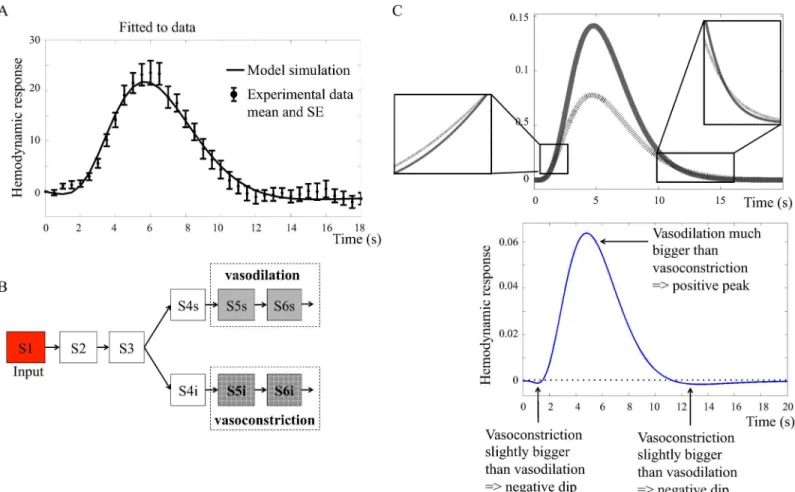
Fig 6. A. Neurotransmitter feed-forward modelMn1ðbp6Þfitted to data.Thefigure shows mean values and standard error (SE) from primary stimulus in
the intensity experiment.B. Interaction graph of the minimized modelMn2.Vasodilating (grey) states contribute positively to the output term and
vasoconstricting (hatched) states contribute negatively. S1. . .S6 are different states in the model. The behavior of these states are represented with the same color coding in C.C. (upper panel) Main mechanism ofMn2.The solid grey line shows the action of the vasodilating terms and the black hatched
line shows the behavior of the vasoconstricting terms. The insets show the small, but essential, differences that give rise to the initial dip and the post-peak undershoot.C. (lower panel) Resulting BOLD response fromMn2.The vasodilating states minus the vasoconstricting states give rise to a BOLD
response with initial dip, peak, and post-peak undershoot.
term has a later but quicker rise to high amplitudes, and falls more quickly back to baseline compared to the dilating term.
The neurotransmitter feed-forward model predicts vasoconstriction to cause the initial dip. The neurotransmitter feed-forward modelMn1ðbp6Þcan display all characteristic features
of the BOLD responsei.e.,the initial dip, the peak, and the post-peak undershoot.Mn1ðbp6Þcan
alsofit the estimation data. However, when investigating the biological mechanisms, we observed that the initial dip, according to the model, is caused by a constricting output term that rises earlier than the dilating term. That is to say, the neurotransmitter feed-forward model predicts vasoconstriction to cause the initial dip. As previous research suggests that the initial dip most probably is related to oxygen metabolism [3], we reject the neurotransmitter feed-forward model. However, as both the existence of and the mechanisms behind the initial dip is debated, this issue is further addressed in the Discussion.
The neurotransmitter feed-forward hypothesis is rejected. In summary, the neurotrans-mitter feed-forward model structureMn1can describe the experimental data, and it can
pro-duce an initial dip, peak, and post-peak undershoot. However, it is rejected during the hypothesis testing, because the hypothesis is not biologically plausible, as the initial dip is caused by vasocontraction instead of oxygen metabolism.
An extension of the neurotransmitter model structure fulfills the biological
plausibility criteria
Results described above show that the increased oxygen metabolism in the metabolic feedback hypothesis can produce an initial dip and that the neurotransmitter feed-forward hypothesis can give a realistic description of the blood flow increase during the BOLD response. Therefore, the neurotransmitter model structure was extended with a metabolic module,Mnm1(Fig 7). In
Mnm1, the neuronal activity increases metabolism in the metabolic module and at the same
time triggers glutamate release in the neurotransmitter module. The levels of dHb and oHb are controlled by the metabolic module and the blood flow is controlled by the neurotransmitter feed-forward module.Mnm1has no feedback control of the blood flow. The output of this final
model structure is the ratio of dHb and oHb.
The extended feed-forward model has realistic biological mechanisms. The model structureMnm1bridges the gap between cellular action and the regulation of the BOLD
response on a vascular level. The model structureMnm1can fit data from the primary stimuli in
both experiments, seeFig 8A. As can be seen inFig 8B, the final model has an early and moder-ate glucose metabolism (the glucose level drops about 5% during the first second). InFig 8B, it can also be noted that oxygen drops during the first second while inFig 8Cthe blood flow is stable during the first seconds, indicating that oxygen metabolism causes the initial dip. The blood flow causing the peak and undershoot is controlled by the neurotransmitter feed-forward module (Fig 8C, peak at 6 s).
Minimization of the extended neurotransmitter feed-forward model structure. The extended model structureMnm1represents the system described in Atwellet al.[16] and
con-tains the key biological elements described there. However, the model structure ofMnm1can be
simplified without loosing the essential mechanisms of the neurovascular coupling. Therefore,
Mnm1was minimized to the minimal model structureMnm2(seen in Fig H inS1 Appendix).
The minimization was done by removing the parallell pathways controlling vasodilation and other key biological elements, with the criterion thatMnm2pass both the the likelihood ratio
and theχ2test. If any more such states were removed, the cost of the model fit increased
drasti-cally and the model passed neither the likelihood ratio nor theχ2test. The 49 parameters of
11.2 for the primary stimulus of the intensity experiment and 7.2 for the primary stimulus of the frequency experiment. The lowest cost for the minimal model structureMnm2in the same
experiments were 27.5 and 18.8, respectively. Cutoff for the likelihood ratio test was 33.9 (df = 22), and thus the model structureMnm2passes the likelihood ratio test despite the
decreased number of parameters. The minimal model structureMnm2does not separate
between neurons and astrocytes, but retains only the principle of a dilating and a constricting arm controlling the blood flow. Just as inMnm1before the minimization, increased oxygen
Fig 7. Interaction graph of the extended model structureMnm1.The model structure has two modules: the neurotransmitter module, which controls the
blood flow, and the metabolic module, which controls the oxygen and glucose metabolism. Whole squares = states, dashed squares = variables (dependent on states), whole arrows = transformations, dashed arrows = interactions, green area = astrocyte, blue area = neuron, grey area = blood. All states starting with S and a number (e.g S2PG) are delay states. Stimulus = input signal. oHb and dHb are oxyhemoglobin and deoxyhemoglobin, respectively.
Glu = glutamate, Calcium neuron and calcium astrocyte = calcium ion (Ca2+) level in the cell, NO = nitric oxide, cGMP = cyclic guanosine monophosphate, AA = arachidonic acid, EET = epoxyeicosatrienoic acids, PG = prostaglandins and 20—HETE = hydroxyeicosatetraeonic acid. All terms starting with k (e.g k1), are parameters and in most cases represent rate constants. PL is a parameter representing phospholipase A2, which is present in abundance. Gbody, O2body, oHbbody and dHbbody, are variables representing the glucose, oxygen and hemoglobin delivered into the area.
Fig 8. A. The model structureMnm1ðbp7Þfitted to data. Thefigure shows mean values and standard error
(SE) from primary stimulus in the intensity experiment. Here the model was forced to display an initial dip and a post-peak undershoot.B. Glucose and oxygen inMnm1ðbp7Þ.Reduced, but not depleted, glucose level
triggers bloodflow increase. The increased oxygen metabolism after stimulus causes the initial dip.C. Vasoconstrictive inhibition of bloodflow during the initial dip does no longer occur.
metabolism causes the initial dip inMnm2, while the blood flow remains stable during the first
seconds after the stimulus.
Predictions of the intensity and frequency experiment validation data. In order to fur-ther test the model structuresMnm, we made core predictions of the BOLD responses to all
sti-muli in the intensity and frequency experiments according to the model construction work flow described inFig 1C, Step 5, and validated the core predictions with the new data (Fig 1C, Step 6).Fig 9shows that the intensity experiment validates the predictions of both the extended modelMnm1ðbp7Þand the minimized modelMnm2ðbp8Þ. BOLD responses from the intensity
experiment were simulated by changing the amplitude of the input. As the true experimental stimulation intensity for the three types of stimulation (white, light grey and dark grey circles) were not known, only the qualitative behavior of the BOLD response was predicted. Both model structures predict decreased BOLD response peak amplitudes in response to a decreased input signal (Fig 9B and 9C, middle and right panels). Experimental data (Fig 9B and 9C, left panels) confirmed this prediction and indicated that visual stimuli with lower intensity had
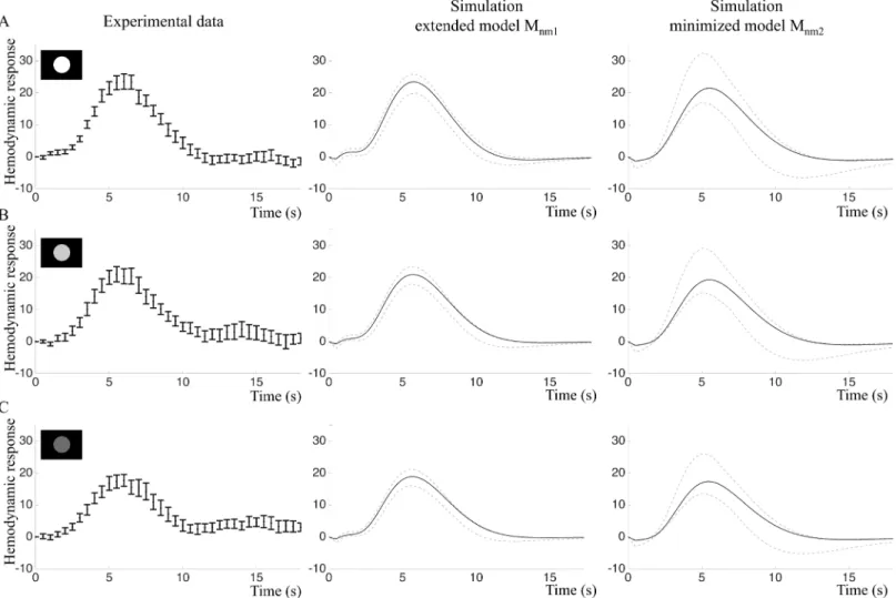
Fig 9. Intensity experiment: Fitting and predictions of the extended modelMnm1and the minimized modelMnm2.A. Left: Estimation data (mean and
SE) of the primary stimulus in the intensity experiment. Middle and right: Model simulations optimized to the estimation data. Black lines represent the best fit and grey lines represent the maximal or minimal value at that time point from a representative selection of acceptable parameter sets. B. Experimental validation data (left) and core predictions (middle and right) for the light grey stimulus. C. Experimental validation data (left) and core predictions (middle and right) for the dark grey stimulus.
lower amplitudes of the BOLD response. However, this decrease was not statistically significant for our small sample,p= 0.058 in repeated measures ANOVA (Fig 9, right panels). The white stimulus resulted in the highest mean amplitude, 25.5 au (sd = 7.4) and the dark grey stimulus in the lowest mean amplitude, 20.1 au (sd = 8.2).
In the frequency experiment, the amplitude of the input signal is constant but the stimuli are repeated with 1 s or 4 s IPI. Here, quantitative traits of the data were also predicted. To account for changing basal conditions, the model was re-optimized and the time course from the primary stimulus in the frequency experiment (Fig 10A, left panel) was used as estimation data, yieldingMnm1ðbp9ÞandMnm2ðbp10Þ.
For paired stimuli with 1 s IPI, both models predicted a single BOLD response peak with higher amplitude compared to the single stimulus (Fig 10B, middle and right panel). For paired stimuli with 4 s IPI, the extended modelMnm1predicted a BOLD response doublet with
approximately the same amplitude as the single stimulus (Fig 10C, middle panel), while the minimized modelMnm2predicted that the second peak should be higher than the first (Fig 10C, right panel).
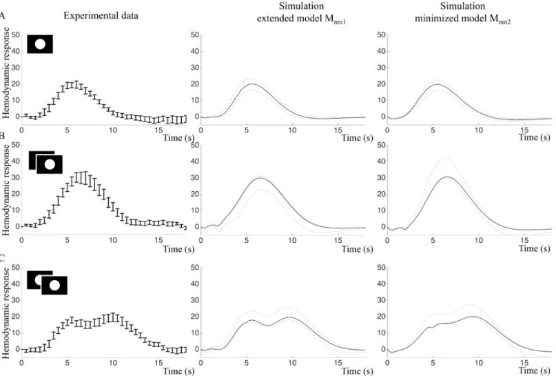
Fig 10. Frequency experiment: Fitting and predictions of the extended modelMnm1and the minimized modelMnm2.A. Left: Estimation data (mean
and SE) of the primary stimulus in the frequency experiment. Middle and right: Model simulations optimized to the estimation data. Black lines represent the best fit and grey lines represent the maximal or minimal value at that time point from a representative selection of acceptable parameter sets. B.
Experimental validation data (left) and core predictions (middle and right) for the 1 s IPI stimulus. C. Experimental validation data (left) and core predictions (middle and right) for the 4 s IPI stimulus.
The core predictions were then compared to experimental data. The paired stimulus with 1s IPI resulted in a BOLD response with one peak, while the paired stimulus with 4 s IPI produced a BOLD response doublet where the peaks were of approximately equal hight (Fig 10B and 10C, left panels). The 1 s IPI stimulus resulted in a BOLD response with a significantly greater mean amplitude, 33.1 au (sd = 12.8) than the mean amplitude of the single stimulus response, 22.7 au (sd = 7.8),p= 0.005 in two-tailed paired t-test. Statistically, both models were able to predict the 4 s IPI data, but as can be seen inFig 10C, the predictions of the extended model
Mnm1has a shape more similar to the validation data compared toMnm2.
Discussion
We have presented mathematical modeling of the mechanisms underlying the BOLD response in fMRI, based on the metabolic feedback and the neurotransmitter feed-forward hypotheses, extensively discussed in the literature [15][16][29]. These hypotheses describing the funda-mental mechanisms behind the BOLD response have, to our knowledge, not been mechanisti-cally modelled before using systems biology approaches. Such approaches provide new tools to evaluate the influence of different hypotheses of the neurovascular coupling causing the BOLD response.
The metabolic feedback model structuresMm1,Mm2, andMm3have problems fitting the data
(Fig 11). The model structures also have problems with simulating the characteristic traits of the BOLD response, (i) the initial dip, (ii) the peak, and (iii) the post-peak undershoot, at the same time. Further, none of the metabolic feedback model structures could describe a biologically plausible time course of the glucose state (Fig 5). The neurotransmitter feed-forward model structure could describe the data and the characteristic traits, but lacked mechanisms for a cor-rect description of oxygen metabolism as the driving force of the initial dip. Of the model struc-tures tested herein, only the model strucstruc-turesMnm1andMnm2that combine neurotransmitter
control over the blood flow with glucose and oxygen metabolism can fully describe the BOLD response. The model structureMnm1could also predict the BOLD responses triggered by stimuli
in the intensity and frequency experiments that were not present in the estimation data. Based on these results, we argue that an addition of metabolism to the neurotransmitter feed-forward hypothesis explains necessary mechanisms generating the BOLD response.
We will now discuss the biological interpretation and the underlying assumptions of the model structureMnm1.
Initial dip
The initial dip is stated as a biological criteria that the model must be able to perform in order to be accepted. The existence of the initial dip is debated [4][5]; it has been observed in some studies [30][31], but not in others, at least not in all subjects [30][32]. Several factors can explain the absence of an initial dip in experimental data: (1) The initial dip is reported to be only 1–2% of the baseline signal [30][31]; in other words, given the low signal to noise ratio in fMRI, the shallow dip could easily be undetected. (2) The intersubject variability is considerable in fMRI [33][34], and thus, the subject selection could be decisive for observing an initial dip or not. (3) The observance of an initial dip could be dependent on the experimental design. For instance, Huet al.[30] found that the magnitude of the dip was reduced for brief stimuli; the minimum stimulus duration in their study was 1.5 s, and we used a duration of only 0.5 s, which could possibly explain the absence of the initial dip in our study. Even though the data largely lacked the initial dip, we included the initial dip as a constraint in our models.
metabolism leads to increased dHb levels and following decreased early-phase BOLD response. This hypothesis has been described previously by a model using the gamma variate curve [13], and is also supported by optical imaging studies showing early stimulus-related dHb increases [35][36]. Based on these previous studies and the simulations of the metabolic feedback model structure in our work, the oxygen metabolism (but not the feedback) of the metabolic feedback hypothesis is necessary, but not sufficient, to reproduce the shape of the BOLD response. How-ever, the metabolic feedback model structure has difficulties explaining the initial dip in combi-nation with a post-peak undershoot (seeFig 5). The neurotransmitter feed-forward model structure, on the other hand, predicts an initial dip caused by initial vasoconstriction, a predic-tion that is not supported by any previous data (e.g.[4][5]) leading to rejection of that model structure. According to our extended model structure,Mnm1, the initial dip is caused by
changes in dHb/oHb ratio due to increased oxygen metabolism occurring during a CBF delay period, as described above.
BOLD response peak
The most noticeable feature of the BOLD response is the large stimulus-induced peak of the fMRI signal. Originally it was suggested that reduced blood-oxygen levels increased the CBF
Fig 11. Schematic diagram of rejections and acceptances of the different model structures evaluated in the present study.Only the final models Mnm1andMnm2fulfill all criteria.✓= model passes the test, X = model fails the test, - = test not applicable or not performed because the model failed a
previous tests.
[1], and consequently the fMRI signal. This suggestion formed the basis for the model structure
Mm1. However, we showed that the oxygen-triggered feedback cannot cause such large
over-shoot (Fig 5A). Later on, Foxet al.[15] showed that CBF and CMRO2correlate strongly in the
brain at rest, but not in response to stimuli; they found that CBF increased by 50%, CMRgluby
51%, but CMRO2only by 5% when the brain is activated. They also concluded that the brain
metabolism is aerobic during rest and anaerobic in response to stimuli, to cover the excess energy needed, which is reflected later in the astrocyte-neuron-lactate-shuttle model proposed by Magistretti and Pellerin [37]. Foxet al.[15] also showed that regional CBF is not driven by oxidative metabolism, but that stimulus-induced CBF is driven by increased glucose demand (see review by Paulsonet al.[29]). Prichardet al.[38] hypothesized that aerobic glycolysis might be close to its maximum capacity in the resting brain. Therefore, stimulus-induced activ-ity requires quick energy increases via anaerobic glycolysis, causing the uncoupling of glucose and oxygen metabolism and CBF.
In line with previous experimental research [15][29], we show that if metabolism is the driv-ing agent for stimulus-induced CBF then blood flow needs to be controlled by glucose, and stimulated metabolism must be partly anaerobic to obtain both an initial dip and a peak in the BOLD response. However, we also show that the metabolic feedback model structuresMm2
andMm3overstate predicted glucose reduction in response to stimuli, as they predict almost
total depletion of glucose to trigger CBF feedback leading to rejection of the metabolic feedback model structure,Mm. This suggets that the metabolic feedback hypothesis plays a limited, if
any, role in the neurovascular response, a conclusion supported by results from Lindauer et al. [39] and Wolf et al. [40] who showed that an increased CBF response will still occur even when hemoglobin is fully oxygenated and that CBF remains unchanged at hypoglycemia.
The neurotransmitter feed-forward model structureMnsuggests that CBF is regulated in
response to neuronal signaling itself and determined by the intensity and duration of the input signal. In our work,Mnpredicts all characteristic features of the BOLD response and has
acceptable fit to data. By minimizing the model, we could show that the main mechanism in
Mnis a balance between vasoconstriction and vasodilation. One caveat with the
neurotransmit-ter feed-forward model is that it predicts vasoconstriction to cause the initial dip, as discussed above.
According to the final model structureMnm1, which has neurotransmitter control of the
blood flow combined with metabolism of glucose and oxygen, CBF is primarily controlled by neurotransmitters that initiate processes in neurons and astrocytes causing release of vasoactive agents. The final model also predicts glucose response with similar shape as post-stimulus glu-cose levels measured by optical methods in rat [41] (Fig 8).
Post-peak undershoot
The final characteristic of the BOLD response is the post-peak undershoot. According to our final model structure,Mnm1, the post-peak undershoot is dependent solely on
neurotransmit-ter-triggered changes in CBF. This result is supported by previous literature that suggests that the post-peak undershoot is caused by a post-stimulus CBF undershoot ([42][43][44] reviewed in [3]). In our data, the post-peak undershoot appears in most of the individual data sets. How-ever, the undershoot seems to become deeper as the peak grows higher in the intensity data sets, and the models tested in the current work cannot predict this behavior. Furthermore, the model cannot describe the deeper undershoot in the 1 s IPI dataset, although it can predict the increased amplitude of the peak.
post-stimulus baseline return of CMRO2-related oxygenation or venous CBV [3]. Mandeville
and coworkers [45] found slow recovery of CBV that matched the post-peak undershoot dura-tion suggesting a biomechanical rather than a metabolic effect [46]. It is worth noting that the balloon model explains the post-peak undershoot as a slow CBV recovery [6]. It has also been suggested that the post-peak undershoot is modulated by post-stimulus neural activity [47] [48]. Future studies incorporating models for CBV changes and/or post-stimulus neural activ-ity might clarify the neurovascular mechanisms behind the post-stimulus undershoot.
Neurotransmitter and metabolic parameters
The neurotransmitter feed-forward model with metabolismMnm1contains several
experimen-tally undetermined parameters, such as glutamate and glucose levels. In future studies, the model parameters can be evaluated and optimized using magnetic resonance spectroscopy (MRS) in combination with BOLD-fMRI. In proton MRS, it is possible to obtain time-depen-dent variations of the neurotransmitters glutamate and GABA and metabolites such as glucose and lactate [49][50][51]. In these recent high-field (7 T) MRS studies, it has been shown that glutamate, GABA, and lactate levels increase during visual stimulation and motor activation, whereas the glucose levels decreases during the same period. If volume was added to the model, a closer estimation of some parameters would also be possible, using experimental values from current literature. This would open the door to prediction of parameter values, in addition to the current predictions of model behaviour.
Assumptions and limitations
As with all models, the model structures evaluated in this work depend on a number of under-lying assumptions, which in turn limit the conclusions that can be drawn from the results. Nev-ertheless, such assumptions are essential in order to build a comprehensible model. We are well aware that there are several different hypotheses of the mechanisms behind specific fea-tures of the BOLD response, of which some are described above. In this work we chose to focus on two fundamental hypotheses.
In the final model structure,Mnm1, the metabolic and the neurotransmitter module run in
parallel. One of the consequences of this structure is that the metabolism is directly controlled by the input signal (seeFig 7). A more physiologically relevant model would be to integrate the metabolism into neurons and astrocytes. That is to say, to model the glycolysis and oxidative metabolism as actually occurring in the neuronal cells in response to stimuli.
Another part of the model structure that lacks physiological details is the action of smooth muscle cells and effects of cortical vessel elasticity. These mechanisms are in our model repre-sented by delay states, which will not accurately represent the possible non-linearities of recep-tor actions and muscular contraction or relaxation. In addition, the current model does not differentiate between capillaries and arterioles. Recent research has found that cerebral hemo-dynamics has a spatiotemporal dependence related to the effective blood viscosity and cortical vessel stiffness [52] and mechanical restrictions on blood vessels depending on cortical depth [53]. A compartmentalized model that takes spatiotemporal hemodynamics into account would provide a physiologically more accurate description of the BOLD response.
Finally, the output signal of the model is oHb/dHb, a simplification suggested by Ogawa
et al.[1]. However, the BOLD signal equation provides a more correct description of the output signal.
DS S0
¼e DR2TE 1 DR
whereS0is the MR signal at baseline andΔSis the BOLD signal change with activation.DR2is
the difference in transversal relaxation rate between the activated state and baseline.DR
2is
lin-early related to dHb concentration. Following ideas from Daviset al.[54], several improve-ments of the BOLD signal description have been published [8][55][56]. In the current work, volumes are not included in the model and therefore it is not possible to implement an output dependent on dHb concentration. However, by dividing the model into a tissue compartment and a blood compartment, as has been done ine.g.[13], a more realistic expression for the out-put BOLD signal can be obtained.
Balancing complexity and overfitting against ability to predict data
When comparing models with each other, it is important to keep track of model complexity and watch out for potential problems with overfitting. We approach these issues first by choosing a model framework not designed to be as flexible as possible, but instead based on the actual mech-anisms believed to be present in the system. Second, we do visual inspection of the plots compar-ing data and model fits (Figs9Aand10A). As can be seen in bothFig 9A and 9B, in the time-window 12–18 seconds the mean values in the data show minor fluctuations, which most likely are noise. The model is not following these minor variations, which argues that we do not have problems with overfitting. Nevertheless, in the early time-points (t = 0–3 s), the extended model does an initial dip, stays down a while, and then rises. Since a similar delayed rise can be seen in the data, this could in principle be a sign of overfitting. However, our third approach to test for overfitting—core prediction analysis—argues against that. In the core prediction analysis, we study a representative sub-set of all parameters that describe the data in a statistically acceptable way. In other words, since the core prediction analysis includes both optimal and less optimal parameters, it does not matter if there are some parameters that are overfitted, as long as parame-ters that are not overfitted are included in the prediction uncertainty analysis. Furthermore, this core prediction analysis shows that all found parameters show an initial dip and a delay (Figs9A
and10A, middle columns), arguing that this property is a necessary consequence of the model structure and the data, i.e. a uniquely identified core prediction. Our fourth approach for check-ing for unnecessary over-parametrization is model minimization. This punishes for unnecessary complexity in the sense of parameters that can be removed without significantly worsening the agreement with the estimation data (Figs9Aand10A, middle and right columns). Finally, the perhaps most important approach to check for overfitting is to use independent validation data. As can be seen in Figs9B, 9Cand10B, 10C, both the extended model (middle columns) and the minimized model (right columns), agree with this independent data, to which they have not been fitted. Furthermore, as can be seen in e.g.Fig 10C, the original extended model actually agrees slightly better with the data than the minimized model. All these facts argues that our models—although over-parametrized in the sense that many parameters have non-unique val-ues—still are based on realistic biological mechanisms that capture the main features seen in the data, and not on too flexible model structures that are fitting to a specific noise realization.
Conclusions
Although the BOLD response has been extensively studied and systems biology is a well estab-lished method, no one has so far investigated the BOLD response using this type of modeling. In this article, a model based on current physiological hypotheses of the mechanisms behind the BOLD response is presented. The model structuresMnm1andMnm2can describe the time course
Systems biology opens the door to a new type of fMRI analysis, which is firmly based in the physiology of the neurovascular coupling behind the measured signal. Systems biology also gives us the opportunity to obtain information about neural activation beyond what we can measure and may thereby help deepen our understanding of the complex system that is the brain.
Supporting Information
S1 Appendix. The S1 Appendix contains interaction graphs, equations and parameter val-ues for all models presented in this article.It also contains graphs showing the fit of the mod-elsMm1andMn2as well as the simulated glucose behaviour in the modelMnm1.
(PDF)
S2 Appendix. The S2 Appendix contains the BOLD response time series (group mean and SE) from all experiments used in this manuscript.
(TXT)
Acknowledgments
We thank Dr Suzanne T. Witt for valuable discussions regarding fMRI image analysis and the test subjects for donating their time in the scanner.
Author Contributions
Conceived and designed the experiments: KL ME. Performed the experiments: AS FL. Ana-lyzed the data: KL SS AS FL. Contributed reagents/materials/analysis tools: ME GC. Wrote the paper: KL SS FE AS FL GC ME. Conceived and designed the study: ME GC KL FE.
References
1. Ogawa S, Lee TM, Kay AR, W TD. Brain magnetic resonance imaging with contrast dependent on blood oxygenation. Proc Nat Acad Sci. 1990; 87:9867–9872. doi:10.1073/pnas.87.24.9868 2. Logothetis NK, Pauls J, Augath M, Trinath T, Oeltermann A. Neurophysiological investigation of the
basis of the fMRI signal. Nature. 2001; 412:150–157. doi:10.1038/35084005PMID:11449264 3. Kim SG, Ogawa S. Biophysical and physiological origins of blood oxygenation level-dependent fMRI
signals. J Cerb Blood Flow Metab. 2012; 32:1188–1206. doi:10.1038/jcbfm.2012.23
4. Buxton RB. The elusive initial dip. NeuroImage. 2001; 13:953–958. doi:10.1006/nimg.2001.0814 PMID:11352601
5. Hu X, Yacoub E. The story of the initial dip in fMRI. NeuroImage. 2012; 62:1103–1108. doi:10.1016/j. neuroimage.2012.03.005PMID:22426348
6. Buxton RB, Wong EC, Frank LR. Dynamics of blood flow and oxygenation changes during brain activa-tion: the balloon model. Magn Res Med. 1998; 39:855–864. doi:10.1002/mrm.1910390602
7. Friston KJ, Mechelli A, Turner R, Price CJ. Nonlinear responses in fMRI: Balloon model, Volterra ker-nels, and other hemodynamics. NeuroImage. 2000; 12:473–481. doi:10.1006/nimg.2000.0630 8. Buxton RB, Uludag K, Dubowitz DJ, Liu TT. Modeling the hemodynamic response to brain activation.
NeuroImage. 2004; 23:S220–S233. doi:10.1016/j.neuroimage.2004.07.013PMID:15501093 9. Sotero RC, Trujillo-Barreto NJ. Modeling the role of excitatory and inhibitory neural activity in the
gener-ation of the BOLD signal. NeuroImage. 2007; 35:149–165. doi:10.1016/j.neuroimage.2006.10.027 PMID:17234435
10. Glaser DE, Friston KJ, Mechelli A, Turner R, Price CJ. Haemodynamic modelling. Academic Press; 2003.