Contributions at Ecologic Boundaries
Lee-Ann C. Hayek1, Brent Wilson2*
1Smithsonian Institution Mathematics and Statistics NMNH MRC-121, Washington D.C., United States of America,2Petroleum Geoscience Programme, Department of Chemical Engineering, The University of the West Indies, Saint Augustine, Trinidad, Trinidad and Tobago
Abstract
Not all boundaries, whether stratigraphical or geographical, are marked by species-level changes in community composition. For example, paleodata for some sites do not show readily discernible glacial-interglacial contrasts. Rather, the proportional abundances of species can vary subtly between glacials and interglacials. This paper presents a simple quantitative measure of assemblage turnover (assemblage turnover index, ATI) that uses changes in species’ proportional abundances to identify intervals of community change. A second, functionally-related index (conditioned-on-boundary index, CoBI) identifies species contributions to the total assemblage turnover. With these measures we examine benthonic foraminiferal assemblages to assess glacial/interglacial contrasts at abyssal depths. Our results indicate that these measures, ATI and CoBI, have potential as sequence stratigraphic tools in abyssal depth deposits. Many peaks in the set of values of ATI coincide with terminations at the end of glaciations and delineate peak-bounded ATI intervals (PATIs) separated by boundaries that approximate to glacial terminations and to transgressions at neritic depths. These measures, however, can be used to evaluate the assemblage turnover and composition at any defined ecological or paleoecological boundary. The section used is from Ocean Drilling Program (OPD) Hole 994C, drilled on the Blake Ridge, offshore SE USA.
Citation:Hayek L-AC, Wilson B (2013) Quantifying Assemblage Turnover and Species Contributions at Ecologic Boundaries. PLoS ONE 8(10): e74999. doi:10.1371/ journal.pone.0074999
Editor:Vanesa Magar, Plymouth University, United Kingdom
ReceivedMarch 7, 2013;AcceptedAugust 8, 2013;PublishedOctober 9, 2013
This is an open-access article free of all copyright, and may be freely reproduced, distributed, transmitted, modified, built upon, or otherwise used by anyone for any lawful purpose. The work is made available under the Creative Commons CC0 public domain dedication.
Funding:These authors have no support or funding to report.
Competing Interests:The authors have declared that no competing interests exist. * E-mail: [email protected]
Introduction
Biostratigraphers historically have sought means to subdivide the sedimentary stratigraphic record as finely as possible. There is, however, evidently a limit to the zonal resolution that can be attained using a single fossil group [1]. For example, the majority of the Pleistocene, the base of which is placed at 2.588 Ma [2], is currently ascribed to the Globorotalia truncatulinoides truncatulinoides (dOrbigny) planktonic foraminiferal Zone [3] or to Zones PT1a and PTIb based on planktonic foraminifera [4] (author names are given at the first mention of any species).
It has long been appreciated, however, that glacial and interglacial fauna and flora within the Pleistocene differ [5], both on land [6] and in the oceans [7]. In Chile, for example, plant leaf architecture changes from a mixture of species belonging to the cool temperate North Patagonian Forest and more thermophilous rain forest vegetation between glacials and interglacials [8]. Glacial-interglacial contrasts in the insect community have been recorded in Greenland [9]. Such changes have been recorded among some foraminifera, but not at all sites. Schott [10] found thatGloborotalia menardii(d’Orbigny) in the Indian Ocean was more abundant in interglacial than in glacial sediments. Phleger et al. [11], in a study of North Atlantic foraminifera, noted the presence in piston cores of ‘‘layers of faunas normal for their latitude alternating with faunas typical of a higher latitude,’’ while Bandy [12] was able to distinguish glacials from interglacials off southern California using the ratio between populations of sinistrally and dextrally coiled Neogloboquadrina pachyderma (Ehrenberg). Streeter
[13] found that Atlantic benthonic foraminifera at depths .2500 m varied greatly over the last 150 ka and suggested that this arose because of depression and elevation of faunas through a depth range of several hundred meters between glacials and interglacials [14]. Streeter and Lavery [15] recorded that uppermost Pleistocene faunas in cores from the western North Atlantic slope and rise north of 35uN were dominated byUvigerina, but that Hoeglundina dominated in the Holocene. This faunal transition was apparently diachronous, occurring at ,12 ka at
3,000 m, but at,8 ka at 4,000 m. Thomas et al. [16] examined
benthonic foraminifera in two lower bathyal (,1700 m) and
abyssal (,3500 m) piston cores spanning the last 45 ka in the
to increased annual primary production. Gaby and Sen Gupta [19] found glacial and postglacial assemblages of the abyssal Venezuela Basin to differ, the Holocene fauna containing abundant Cibicides wuellerstorfi (Schwager), Melonis pompilioides (Fichtel and Moll), Nuttallides umbonifera (Cushman), and Pullenia sp., while the fauna in the last glacial was dominated byMassilina sp., Globocassidulina subglobosa (Brady) and Nummoloculina irregularis (d’Orbigny).
Glacial-interglacial contrasts in the benthonic foraminiferal fauna are not everywhere marked, however. Streeter and Lavery [15] wrote that on the western North Atlantic continental rise below 4,000 m, ‘‘the glacial to modern faunal shift is subtle, but it clearly occurs later than on the upper rise.’’ Sen Gupta et al. [20] examined benthonic foraminifera over the past 127 ka in three bathyal cores (depths near 2000 m) from the western Grenada Basin, eastern Caribbean Sea. They found only subtle changes, rather than drastic turnovers, at glacial-interglacial boundaries based on the abundance ofGloborotalia menardii. They stated that neither species richness S nor the information function H~{Ppi:ln (pi), where pi is the proportional abundance of
theith species) showed any distinct stratigraphic trend (although H is not expected to show such a trend [21]). However, they suggested Nuttallides umbonifera, Bulimina buchiana dOrbigny and Chilostomella oolinaSchwager to be rarer in the last glacial than in the two bounding glacials. Wilson [22,23] examined the benthonic foraminifera in two bathyal piston cores near the northern Leeward Islands, eastern Caribbean Sea. He did not find any marked faunal changes at the Pleistocene-Holocene boundary, but showed that the organic flux in one core decreased gradually through the entire core. Wilson [24] found only weak evidence of Milankovich cycles in the Upper Quaternary of ODP Hole 1006A (Santaren Channel, offshore western Bahamas), where Globocassi-dulina subglobosaandCibicidoides aff.C. io(Cushman) were smaller assemblage components during most glacial MISs. However, the percentages of these species varied between odd-numbered MISs and they were insignificantly correlated with one another, G. subglobosabeing rare in MIS 9 whileC. aff.C. iowas common.
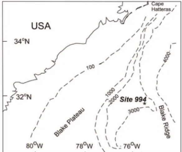
The inability to detect glacial-interglacial contrasts at all sites appears to arise because not all sites show marked changes in community composition at the species level at glacial-interglacial boundaries. Rather, the proportional abundances of species vary between glacials and interglacials to differing degrees. This paper presents a simple quantitative measure, the assemblage turnover index (ATI), which uses changes in species’ proportional abundances to identify intervals of marked community change. Whittaker [25] distinguished two categories of diversity: inventory diversity, which calculates the diversity of associations within samples (point diversity) or habitats (adiversity); and differentia-tion diversity, which examines the change in diversity between samples (pattern diversity) or habitats (bdiversity). The assemblage turnover index presented here is a form of differentiation diversity. A conditioned-on-boundary index (CoBI), developed as a function of the ATI, identifies species that contribute most to maxima and minima in sets of values of the ATI. The section used in this demonstration is from Ocean Drilling Program (OPD) Hole 994C, drilled on the Blake Ridge, offshore SE USA (Figure 1). Although Bhaumik and Gupta [26,27] and Mohan et al. [28] have examined Neogene benthonic foraminifera from this and nearby ODP Holes, glacial-interglacial contrasts have not been recorded at the Blake Ridge before this study.
Site Description
ODP Site 994 (31u47.1399N, 75u32.7539W; water depth 2799 m) is situated on the sediment drift deposit that forms Blake Ridge [29,30], a drift deposit consisting of current-lain sediment east of the Blake Plateau. The Blake Ridge was deposited by the Western Boundary Undercurrent, this being a thermohaline-induced contour current (a current that flows parallel to bathymetric contours), which flows southward along the U.S. continental margin [31]. The Western Boundary Undercurrent transported clays eroded from eastern North America north of 40uN, at least as far south as Puerto Rico [32]. ODP Hole 994C cored a 700 m-thick succession of clays with calcareous nannofossils within which there are no obvious depositional hiatuses [30]. In this paper we examine the topmost
,14 m of sediment in ODP Hole 994C. Mass sediment
transport complexes are absent. The studied section, which is a distinct lithostratigraphic unit termed Unit 1 [30], consists of light gray to gray and greenish gray nannofossil-rich clays in beds up to 1.20 m thick. The presence of the trace fossil Zoophycos indicates that some bioturbation has taken place, but mostly at bedding planes. Biostratigraphic correlation within the Quater-nary of ODP Hole 994C is limited. Okada [33] found the first occurrence of Emiliania huxleyi (Lohmann) at 8.05–9.05 meters below the seafloor (mbsf), between OPD Hole 994C Core 2H-3, 65 cm and 2H-4, 15 cm, for which he suggested an age of 0.26 mya. This indicates a depositional rate of 3.5 cm/ka in the uppermost part of the Hole. The first appearance of E. huxleyi has subsequently been placed between 0.262–0.264 Myr [34].
Bhaumik and Gupta [27] studied the benthonic foraminifera in nearby ODP Hole 997A, and foundBrizalina paula(Cushman and Cahill),Cibicidoides kullenbergi(Parker),Uvigerina hispidocostata Cush-man and Todd andUvigerina peregrinaCushman to be abundant in that part of the section within the gas hydrate zone. Bhaumik and Gupta [26] examined benthic foraminiferal assemblages (.125 mm size fraction), the information function H and total organic carbon in Hole 997A during the late Neogene (last 5.4 Ma). They concluded thatB. paula, Cassidulina carinataSilvestri, Chilostomella oolina, Fursekoina fusiformis (Cushman), Globobulimina pacifica Cushman,Nonionella auris (d’Orbigny) andTrifarina bradyi are potential methane seep-related foraminifera, while U. hispidocostata, U. peregrina, U. proboscidea (Schwager) and Melonis barleeanus (Williamson) indicate a high organic carbon flux independent of deep-sea oxygenation.
Materials and Methods
Sixty seven samples of 20 cm3 were taken at 20 cm intervals from ODP Hole 994C, Cores 1 and 2, between 0.08–13.25 mbsf. They were provided by the Ocean Drilling Program (ODP) that is sponsored by the U.S. National Science Foundation (NSF) and participating countries. The cored site being in international waters, no specific permissions were required for these locations/ activities. The material comprising fossils, sampling did not involve endangered or protected species. Each sample was
,2 cm thick and represents,600 years. Samples were soaked in
water until disaggregated, washed over a 63mm mesh to remove silt and clay, and dried over a gentle heat. An attempt was made to pick N = 250–300 specimens of benthonic foraminifera from the .63mm fraction from each sample. However, only 42 samples yielded .250 specimens (mean, 251 specimens per sample, minimum 104). The methods on assemblages used here have been reported by Wilson [35]. The foraminifera were sorted into species and identified using Cushman [36,37,38,39,40,41,42], Cushman and Henbest [43], Phleger and Parker [44], Phleger et al. [11], Parker [45], Pflum and Frericks [46] and Mohan et al. [28]. The number of specimens (ni) was recorded for each species or species group (i.e., rare
species in the same genus that were left in open nomenclature and grouped together).
Elphidium excavatum (Terquem), Epistominella takayanagii Iwasa, Quinqueloculina poeyana d’Orbigny and Quinqueloculina ex gr. lamarckiana d’Orbigny, which are typical of neritic water, were regarded as allochthonous and excluded from this analysis. Elphidiumis typically regarded as a shallow-water genus [47] that has to be removed from data sets of studies of bathyal foraminifera [48]. Sen Gupta and others [49] recorded abundantE. excavatum on the Louisiana continental shelf. In the southern North Sea, it dominates the foraminiferal fauna at depths between 25–30 m [50].Epistominella takayanagiihas been recorded from Chaleur Bay eastern Canada, mostly in waters ,100 m deep [51], and may have been transported southwards to ODP Site 994C. The proportional abundance of both E. excavatum and E. takayanagii peaked in MIS 10, glacial cycle E, as did the percentage of overall allochthonous, shallow-water species. A single specimen of Stilostomella lepidula (Schwager) recovered from 5.45 mbsf was presumed to be reworked, this species having gone extinct during middle Pleistocene times [52], and was excluded from further analysis. This left a presumed predominantly in situ abyssal assemblage, within which there may have been some slight downslope transport ofAngulogerina occidentalis(Cushman),Bulimina aculeatad’Orbigny,B. alazanensisCushman,Cibicidessp.,Fursenkoina fusiformis (Williamson), Globocassidulina obtusa (Williamson) and Nuttallides rugosa(Phleger and Parker) [35]. This presumed in situ assemblage forms the subject of the remainder of this paper. To examine turnover of an entire assemblage quantitatively across a delineated boundary we developed the ATI index. For a set of samples from a given site, the Assemblage Turnover Index for each pair of adjacent samples is defined as
ATI~jpi2{pi1j ð1Þ
in which pi1and pi2are the proportional abundances of theith
species, i = 1,…, s, in the lower and upper samples (see Appendix S1 for a glossary of terms). This assemblage turnover index between samples will be denoted as ATIs. Note that although for
each samplePpi~1, the measure ATIscan be.1. Thus, ATIs
gives the proportion or percent of turnover or change specifically
across a defined or particular boundary. We calculated the mean
x
x, and standard deviation,s, of values of ATIs over all samples
within the core. To develop our control chart we determined all points with ATIswðxxzsÞ, which were then deemed to be positions of major turnover. Oba et al. [53] presented a d18O curve for ODP Hole 994C (see Figure 2). Their samples were taken at irregular intervals (sample spacing 7–49 cm; mean 22.6 cm, sd 10.9 cm). The values ofd18O for the samples used here were interpolated from Oba et al. ’s [53] curve and correlation between ATIsand interpolated d18O was calculated.
Because Oba et al. ’s [53] uppermost sample was taken at 0.14 mbsf, it was not possible to estimate the d18O value for the uppermost sample picked for this study. Point (sample) values of species richness S and the information function H were calculated. Dominance was determined using max(pi), the proportional
abundance of the most abundant species in each sample [54]. We chose to calculate correlations between ATIs, S, H and max(pi)
using the upper (younger) sample in each sample pair.
Peaks in ATIs, those values larger than our designated control
value of ðxxzsÞ, were used to divide the succession into peak-bounded ATIs(PATI-) intervals. These intervals were numbered,
commencing from PATI-1 for the most recent. PATI-1 and the oldest PATI are incomplete, their upper and lower boundaries respectively not being bounded by ATIspeaks.
To assess which species contributed most to the ATI at the PATI boundaries, a conditioned –on-boundary index CoBI was derived. CoBI provides the proportion that each species within an assemblage contributed to the change or turnover specifically across the PATI boundary. For each species at any PATI boundary
CoBI~jpi2{pi1j=ATI ð2Þ
where pij, j = 1,2 are theith species proportions on either side of
the selected boundary of interest and at which the ATI is calculated.
There are two forms of CoBI:
1. Partial conditioned-on-boundary index, CoBIp, in which the
assemblage turnover index ATIs was calculated between the
entire set of samples within the PATI below the ATI peak and the first sample immediately above the peak. In this case, the ATI is designated as ATIp. The value of ATI ( = ATIp) was
substituted into equation (2), as were pi1, the proportional
abundance of theith species in the entire PATI below the peak in ATIp, and pi2, the proportional abundance of thatith species
in the first sample above the peak in ATIs.The proportional
contribution of each species to ATIp was assessed from the
vector of CoBIpvalues at each ATIspeak.
2. Thorough conditioned-on-boundary index CoBIt, in which the
ATI is denoted as ATIt, was calculated between the values in
two complete PATIs separated by the peak in ATIs (see
Figure 2). The value of ATItwas substituted into equation (2),
as were pi1 and pi2, the proportional abundance of the ith
species in the two PATIs separated by the peak in ATIt. The
proportional contribution of each species to the value of ATIt
was assessed from the vector of partial CoBI for each ATIs
peak.
used to detect assemblage change exactly at the boundary between a single PATI and the next contiguous sample.
Results
Assemblage Turnover Index (ATI = ATIs) Between
Samples
Our presumed in situ, abyssal fauna comprised 16,184 specimens in 157 species (see File S1), and was dominated by Brizalina lowmani (Phleger and Parker) (42.1% of total recovery; range 6.9–70.0% per sample) with subdominant Globocassidulina obtusa (Williamson) (8.9% of total recovery; range 0–21.9% per sample). Thirteen other species formed .1% of total recovery: Bulimina aculeata d’Orbigny, Cassidulina laevigata d’Orbigny, Cibicides wuellerstorfi, Cibicidoides robertsonianus (Brady), Epistominella exigua, Gyroidina lamarckiana (d’Orbigny),Hoeglundina elegans (d’Or-bigny),Melonis baarleeanus(Williamson),M. pompilioides(Fichtel and Moll), Oridorsalis umbonatus (Reuss), Pullenia bulloides (d’Orbigny), Pyrgo lucernula(Schwager) andUvigerina hispidocostataCushman and Todd. The distributions of selected species are shown in Figure 3. The assemblage turnover index between adjacent samples ranged from ATIs = 0.263–1.421(x¯ = 0.710,s= 0.233) (Figure 2),
indicating total assemblage change from 26% to 142%. The value of ATIsexceeded x¯+s= 0.943 across nine pairs of samples. We
chose to include the borderline value of ATIsat 9.85 mbsf, where
it nevertheless formed a pronounced peak. We computed correlations of ATI with the indices H and max (pi) and with d18O. Although the formulae for these measures utilize the relative abundances, there is no linear functional relationship among them that necessitates a significant correlation. The ATIs
was positively correlated with the information function H for the younger sample in the pair (r = 0.62, p,0.0001). ATIs was
negatively correlated with max(pi) (r = –0.65, p,0.0001), which
indicates a change in dominance across peaks in ATIs, and
negatively correlated withd18O (r = –0.32, p,0.01). H andd18O
were in turn significantly negatively correlated (r = –0.53, p,0.0001).
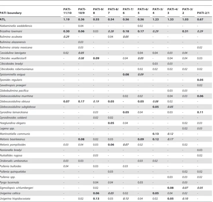
Partial Conditioned-on-Boundary Index (CoBIp)
The accepted peaks in the ATIsdelimited eleven peak-bounded
ATI intervals (PATI-). These intervals contained between one (PATI-3 and PATI-4) and fifteen (PATI-5 and PATI-10) samples. The ATIpused for CoBIpranged between 0.83–1.33 (PATI-6/5
and PATI-4/3 boundaries respectively; Table 1), which indicates assemblage turnover between 83% and 133% at the boundaries. Only 31 species showed CoBIp.0.02 (i.e., accounted for.2% of
ATIp) at any one PATI boundary (Table 1) and these species
differed over the PATI boundaries.
Thirteen species had a CoBIp of 0.02–0.05 at any one
boundary, while 18 (,11.5% of all species recorded) had a CoBIp .0.05 across any one PATI boundary. Seven species (Cassidulina laevigata, Epistominella exigua, Eponides regularis Phleger and Parker, Globocassidulina obtusa,Hoeglundina elegans,Pyrgo murrhina(Schwager), Uvigerina celticaScho¨nfeld) had a CoBIp .0.05 across one PATI
boundary only. Two species (Melonis baarleeanus, Uvigerina hispido-costata) had a CoBIp.0.05 across four PATI boundaries.Brizalina lowmanifluctuated most markedly, having the CoBIp.0.05 across
eight PATI boundaries. The maximum CoBIp was 0.47,
indicating 47% change in B. lowmani abundance across the PATI-7/6 boundary. Four other species (Bulimina aculeata,Gyroidina lamarckiana, Melonis baarleeanus, M. pompilioides) had a maximum CoBIp .0.20 across any one PATI boundary. Using CoBIp, Brizalina lowmanidecreased in proportional abundance across the boundaries between PATI-8/7 and 2/1,M. pompilioides between PATI-7/6 and 2/1, andU. hispidocostatabetween PATI-7/6 and 3/2.
Thorough Conditioned-on-Boundary Index (CoBIt)
The ATItused for CoBItranged between 0.36–1.33 (PATI-10/
9 and PATI-4/3 boundaries respectively; Table 2), or an observed
Figure 2.d18O from Obaet al.[53], the information function H, species richness S (graphed as lnS to facilitate comparison with H), max(pi) and between sample assemblage turnover index (ATIs) [from this paper] in the Upper Quaternary, ODP Hole 994C, Blake
total assemblage change ranging from 36% to 133% between the PATI pairs from PATI-1/2 through PATI-10/11. Thirty three species resulted in a value of CoBIt .0.02 (i.e., accounted for .2% of ATIt) at any one PATI boundary. Twenty eight species
contributed to.0.02 of both ATIpand ATIt. Seventeen species
had a CoBItof 0.02–0.05 at any one boundary. Thus, only sixteen
species (,10% of all species recorded) had a CoBIt.0.05 across
any one PATI boundary. The highest CoBItwas 0.31 forBrizalina lowmani, indicating pronounced change in dominance across the PATI-3/2 boundary, while Bulimina aculeatapresented a compa-rable CoBItof 0.29 across the PATI-11/10 boundary. All other
species contributed a maximum CoBIt ,0.20, although the
maxima forGlobocassidulina obtusaandMelonis baarleeanuswere 0.19 and 0.17 respectively. The CoBItforB. lowmaniwas.0.02 across
eight PATI boundaries, while those forG. obtusawere.0.02 across six boundaries and forM. baarleeanusand Cibicidoides robertsonianus across five.
Discussion
The assemblage turnover index is a form of differentiation diversity sensu Whittaker [25]. It is here presented at two scales, of which the end members are (a) ATIs, which corresponds to
Whittaker’s (1972) pattern or between-sample diversity, and (b) ATIt, which is here taken as corresponding to his between-habitat
or b-diversity. ATIs was strongly positively correlated with the
information function H and negatively correlated with max(pi) for
the younger of the samples in the sample pairs used in its calculation. This indicates that assemblage turnover – the sum of the changes in proportional abundances of species – increases with increasing diversity and with decreasing dominance (i.e. increasing equitability).
The correlation between ATIs,and interpolated values ofd18O
was significant and negative (Figure 2). Oxygen isotopes have been used to erect a paleotemperature record of marine isotope stages (MISs) that is reliable back to MIS 16, 650 ka [17], within which odd numbered MISs are interglacials [55] and against which
faunal changes can be compared. Much of the time between MIS 1–12 (the interval examined in this study) consists of 100 ka MIS couplets [56,57]. Broecker and Van Donk [58] grouped the MISs into glacial cycles (segments of two to four MISs) that were separated by terminations (i.e., pronounced boundaries between isotopic maxima and minima). Because warming during deglaci-ation occurs more rapidly than does cooling during the development of glaciation [59], each termination separates a preceding glacial from a succeeding interglacial. MIS 3 being a subdued glaciation, there is no termination between MIS 4 and 3, but Termination T-I occurs between MIS 2 and 1, and T-II between MIS 6 and 5. The interval examined during this study encompasses terminations T-V to T-I, which separated Glacial Cycles F to A (Figure 3). Cheng et al. [60] positioned terminations at the mid-point between the peaks and troughs in the graph of
d18O. However, because the d18O curve for ODP Hole 994C presented by Oba et al. [53] was based on irregularly spaced samples their technique cannot be used here. It does appear, however, that the boundaries between PATI-11/10, 10/9, 7/6 and 6/5 and 2/1 approximate to terminations T-V through T-I, respectively. Thus, the slower onsets of glacials are marked by low levels of turnover, ATIs, while the more rapid transitions to
interglacials are marked by peaks in ATIs. Because the peaks in
ATIsoccurred within terminations, the correlation between ATIs
andd18O is low.
Not all peaks in ATIs detected across our samples coincide
with terminations. The boundary between PATI-9/8 and 8/7 occurred within MIS 8 and indicates an increase in the flux of organic carbon through that glacial MIS. This may reflect increasing efficiency of the plankton multiplier of Woods and Barkmann (1993).
The close grouping of the boundaries between PATI-5 through PATI-1, all of which occurred during the transition from MIS 2 to MIS 1, show this to have been an interval of protracted environmental change at ODP Site 994. Sea level rose by
,120 m during termination T-1 [61], but did so in several
decimeter steps [62]. It is possible that the closely spaced
Figure 3. Percentage abundances of selected species in the Upper Quaternary of ODP Hole 994C, species presented in alphabetical order.A.Bulimina aculeata. B.Brizalina lowmani. C.Cibicides wuellerstorfi. D.Epistominella exigua. E.Melonis baarleeanus. F.Uvigerina hispidocostata. Dashed lines in A indicate positions of Terminations I – V, with ages in ka BP. Dashed lines in B – F indicate boundaries between PATIs 1 to 11. Terminations are indicated by Roman numerals in order of increasing age.
boundaries from PATI-5 through PATI-1 reflect these steps. Brizalina lowmani did not decrease in proportional abundance across all boundaries between PATI-5 through PATI-1, but increased across the PATI-3/2 boundary.
Some data suggest that the changes in the fauna across the peaks in values of ATIs reflect changes in either (a) dissolved
oxygen levels, (b) the organic carbon flux and (c) bottom current strength, although the first two of these factors are frequently correlated [63]. For a paleoenvironmental summary, see Table 3. den Dulk et al. [64] studied benthonic foraminifera under an upwelling system in the northern Arabian Sea. They recognised two groups of foraminifera:
1. Species that prefer high dissolved oxygen and low organic carbon levels: (Bulimina striata, Gavelinopsis lobatula, Chilostomella oolina, Sphaeroidina bulloides, Cibicides ungerianus, Hyalina balthica,
Hoeglundina elegans, Melonis barleeanus, Quinqueloculina spp., Globocassidulina subglobosa and Cassidulina carinata;
2. Species preferring low dissolved oxygen and high organic carbon:Bulimina exilis, Rotaliatinopsis semiinvoluta, Brizalina alata, B. pygmaea, Globobulimina spp., and Buliminasp.1.
The species ofBrizalinaandBulimina, which dominate in ODP Hole 994C, are limited to group 2. de Rijk et al. [65] found that Bulimina aculeata, which dominated in PATI-11 (Figure 3B), lives primarily where the flux of organic carbon exceeds 3 g m22yr21. Melonis baarleeanus(Figure 3E), although placed in group 1 by den Dulk et al. [64], was shown by Qvale and Van Weering [66] to prefer a fine-grained substrate with a relatively high organic carbon content [67]. Mackensen et al. [68] suggested that in the South Atlantic Ocean it prefers seasonally varying productivity. Taldenkova et al. [69] found this species to be more abundant in
Table 1.Partial conditioned-on-boundary index (CoBIp) for peak-bounded ATIs(PATI-) intervals in the Upper Quaternary in ODP
Hole 994C, Blake Ridge.
Boundary
PATI-11/10
PATI-10/9
PATI-9/ 8
PATI-8/ 7
PATI-7/ 6
PATI-6/ 5
PATI-5/ 4
PATI-4/ 3
PATI-3/
2 PATI-2/1
ATI 1.09 0.89 0.88 0.93 0.91 0.83 0.96 1.33 0.95 0.97
Alabaminella weddellensis - - - 0.02
Brizalina lowmani - 0.20 0.35 0.33 0.47 0.27 0.08 - 0.26 0.21
Bulimina aculeata 0.31 - - -
-Cassidulina laevigata - 0.02 - - 0.04 - 0.09 0.03 0.04
-Cibicides wuellerstorfi 0.03 0.05 0.09 0.03 - 0.09 - 0.04 0.02
-Cibicidoides bradyi - - - 0.04 0.03 - 0.03
Cibicidoides robertsonianus - - - 0.03 - 0.02 0.03
-Epistominella exigua - - - - 0.06 - - - -
-Eponides regularis - - - 0.10
Gavelinopsis praegeri - - - 0.03
Globobulimina pacifica - - - 0.03 0.03
-Globocassidulina murrhina - - - 0.04 - 0.02
Globocassidulina obtusa 0.03 0.03 0.02 - 0.09 - - - -
-Globocassidulina subglobosa - 0.04 - - - - 0.07 0.05 -
-Gyroidina lamarckiana - 0.13 - - - 0.05 - 0.03 - 0.22
Gyroidinoides soldanii - 0.03 - - -
-Hoeglundina elegans - - - 0.15 - - - 0.03
Martinottiella communis - - - 0.17 0.12 -
-Melonis baarleeanus 0.27 0.11 - 0.02 0.02 - 0.24 0.17 -
-Melonis pompilioides 0.04 - - 0.21 0.06 - - - 0.08 0.03
Nonionella bradyi - - - 0.02 - - -
-Oridorsalis umbonatus - 0.08 0.05 - - -
-Pullenia bulloides - 0.03 0.04 - - - 0.02 - -
-Pulleniaspp. - - - 0.03 0.03
-Pyrgo lucernula - - 0.05 0.03 - - 0.03 - 0.03
-Pyrgo murrhina - 0.03 - - - 0.06 - - -
-Robertinoides bradyi - - - 0.02 - - -
-Sigmoilopsis schlumbergeri 0.02 - - - 0.08 0.09
-Trifarina angulosa - - - 0.02 - - - 0.03
Uvigerina celtica - - 0.03 0.04 - - 0.07 0.04 -
-Uvigerina hispidocostata - - 0.18 0.09 0.04 0.02 0.04 0.05 0.11
the upper bathyal Holocene of the Arctic Ocean than the latest Pleistocene, and ascribed it to a distal-river group of relatively deep-water species that thrive on slightly altered organic matter and is therefore restricted to areas with periodic delivery of organic matter. Murray [70] noted that M.baarleeanushas been recorded live in all oceans except the Indian Ocean. In ODP Hole 994C this species accounted for.0.02 of the CoBItacross six of the ten
PATI boundaries, and was abundant in the early part of PATI-10 and in PATI-5 and PATI-4. It was rare to absent in PATI-3 through PATI-1. This suggests that seasonality varied through the Late Quaternary at Blake Ridge. Unlike in the Arctic Ocean [69], at Blake Ridge seasonality was much reduced in the Holocene, after termination T-1.
Globocassidulina subglobosa, which is found throughout the Atlantic, Pacific and Southern Oceans (Murray, 2013), has been suggested to be an oxic indicator [71] that prefers an elevated mean organic carbon flux of 15 g m22yr21[72]. This species was abundant in PATI-4 (which equates to a brief episode in the glacial MIS 2). Smart and Gooday [73] examined trends in benthonic foraminiferal abundances along an organic enrichment gradient on the continental slope off North Carolina, eastern Atlantic Ocean. They foundBulimina aculeata andGlobocassidulina subglobosato be equally abundant at all sites, suggesting that these cannot be used as proxies for the organic flux. It is unclear, however, ifGlobocassidulina obtusa and G. murrhinahave the same tolerances.
Table 2.Thorough conditioned-on-boundary index (CoBIt) for peak-bounded ATIs(PATI-) intervals in the Upper Quaternary in
ODP Hole 994C, Blake Ridge.
PATI boundary
PATI-11/10
PATI-10/9
PATI-9/ 8
PATI-8/ 7
PATI-7/ 6
PATI-6/ 5
PATI-5/ 4
PATI-4/ 3
PATI-3/
2 PATI-2/1
ATIt 1.19 0.36 0.55 0.54 0.56 0.56 1.23 1.33 1.03 0.67
Alabaminella weddellensis - 0.04 - - - 0.02 - - -
-Brizalina lowmani 0.30 0.06 0.03 0.28 0.18 0.17 0.29 - 0.31 0.29
Bulimina aculeata 0.29 - - 0.04 0.05 - - - -
-Bulimina alazanensis - 0.03 - - -
-Bulimina striata mexicana - 0.03 - - - 0.02
Cassidulina laevigata 0.02 0.05 - - - 0.04 0.04 0.03 0.04
-Cibicides wuellerstorfi - 0.08 0.09 - 0.04 0.05 - 0.04 0.04 0.03
Cibicidoides bradyi - - - 0.03 0.03 -
-Cibicidoides robertsonianus - - - 0.02 0.02 0.02 0.02 0.02
Epistominella exigua - - - - 0.08 0.09 - - -
-Eponides regularis - - - 0.05
Gavelinopsis praegeri - - - 0.02
Globobulimina pacifica - - - 0.03 0.03
-Globocassidulina murrhina - - - - 0.02 0.02 - 0.04 0.03 0.06
Globocassidulina obtusa 0.07 0.17 0.19 0.05 - 0.05 0.08 0.02 -
-Globocassidulina subglobosa - - - 0.05 0.05 -
-Gyroidina lamarckiana - - 0.03 - 0.05 0.04 - 0.03 - 0.11
Gyroidinoides soldanii - - 0.02 0.02 - - -
-Hoeglundina elegans - - - 0.05 0.04 - - - 0.02 0.03
Lagena spp. - - - 0.02 0.03
Martinottiella communis - - - 0.13 0.12 -
-Melonis baarleeanus - 0.08 0.02 0.03 - 0.09 0.12 0.17 -
-Melonis pompilioides 0.03 0.04 0.03 0.06 0.07 0.02 - - 0.02
-Nonionella bradyi - - - 0.03
Nuttallides rugosa - - 0.03 - - - 0.02
Oridorsalis umbonatus 0.03 0.03 - - - 0.03 0.02 - -
-Pullenia bulloides 0.04 - 0.03 - 0.03 - - - -
-Pullenia quinqueloba - - - 0.03 - - - - 0.02 0.02
Pullenia spp. - - - 0.03 0.03 0.02
Pyrgo lucernula - - 0.04 0.04 - 0.03 - - 0.03
-Sigmoilopsis schlumbergeri - - 0.02 - - - - 0.08 0.07 0.05
Uvigerina celtica - - 0.06 0.05 0.02 - 0.05 0.04 0.02
-Uvigerina hispidocostata - 0.02 0.13 0.03 0.13 0.04 0.02 0.05 0.10
Kaiho [74] suggested that many of the species recovered from ODP Hole 994C are indicative of suboxic bottom waters, although he also suggested that Cibicides wuellerstorfi (figure 3C) andCibicidoides robertsonianusare indicative of oxic water [75]. The abundance of C. wuellerstorfi was relatively high during PATI-6. Altenbach et al. [72] recorded the annual organic carbon flux levels best tolerated by some live benthonic foraminifera. Most species recorded by Altenbach et al. [72] that were also recovered from ODP Hole 994C lived under a flux rate of,2–6 g m22yr21
(Bulimina striata mexicana, C. robertsonianus, Pullenia bulloides, P. quinqueloba). Scho¨nfeld [71] recorded these four species as living infaunally within the sediment at a variety of depths down to 4.5 cm. However, Altenbach et al. [72] recorded liveC. wuellerstorfi primarily at low organic carbon flux rates of 1.5–3 g m22yr21and Oridorsalis umbonatusat 2–3.5 g m22yr21.Cibicides wuellerstorfiis an epiphytal species living on raised substrate particles that prefers active bottom currents [76,77]. CoBItshowed in ODP Hole 994C
thatC. wuellerstorfiwas recovered primarily from PATI-9, 6, 3 and 1, during which the organic carbon flux may have been low, the strength of the Western Boundary Undercurrent enhanced, or both. Altenbach et al. [72] recovered Hoeglundina elegans mainly from areas with a flux rate of 4.5–15 g m22 yr21, although Scho¨nfeld [71] suggested it to be an oxic indicator. The costate speciesUvigerina mediterraneaandU. peregina, which have morphol-ogies comparable toU. hispidocostata, primarily under a carbon flux of 3–9 g m22yr22. Scho¨nfeld [71] recordedU. peregrinaas living mostly at depths of 0–1 cm below the sediment water interface, butU. mediterraneaas occurring down to 6 cm below the interface. Uvigerina hispidocostata in ODP Hole 994C was recovered mainly from PATI-8 and PATI-7, which coincide with MIS 8, for which it could indicate an interval of enhanced organic carbon flux but might also highlight an interlude in which uvigerinids penetrated deeper into the sediment. Schoenfeld and Altenbach [78] found thatUvigerinaspp. in the north-eastern Atlantic Ocean were more abundant during glacial MIS 2 than interglacial MIS 1, and ascribed this to a widespread change from glacial to modern productivity characteristics across termination T-I. MIS 8 is similarly a glacial stage. Seiglie [79] noted B. lowmani to be indicative of high organic carbon levels and Sen Gupta and Strickert [80] found it to be dominant on the continental slope off Florida at depths.100 m, below the Gulf Stream. In ODP Hole
994CB. lowmani, Cassidulina laevigata, Cibicides wuellerstorfi, Melonis baarleeanus,M. pompilioidesandUvigerina hispidocostatahad the highest number of PATI boundaries across which CoBIp.0.02, whileB. lowmani,Cibicidoides robertsonianus,Globocassidulina obtusa,M. baarleea-nus, M. pompilioides, U. celticaand U. hispidocostatahad the highest number PATI boundaries across which CoBIt .0.02. These
indicate that the organic carbon flux, dissolved oxygen levels and bottom current strength varied between PATIs, rather than between glacials and interglacials.
Gooday et al. [81] found Epistominella exigua (Figure 3D to be abundant in well-oxygenated, abyssal water below the oxygen minimum zone of the Arabian Sea. Smart et al. [82] showed that E. exiguacolonises aggregates of phytodetritus and they speculat-ed that this opportunistic, epifaunal species may represent a proxy for seasonal phytodetritus pulses originating from surface primary productivity in open ocean eutrophic areas. They suggested that inputs added over a geologically prolonged period of time would be reflected in peaks ofE. exigua. This species was at its most abundant in PATI-6, having a ATIp.0.05 across the
PATI-7/6 boundary and a ATIt.0.05 across both the PATI-7/
6 and PATI-6/5 boundaries. This implies a brief interlude of enhanced seasonality in MIS 7 and 6, and may be related to a change in surface circulation and the position of the Gulf Stream at that time.
Sequence stratigraphy is the correlation of sedimentary rock successions using key events produced by worldwide changes in sea level [1]. These events are used to divide the succession into packages (systems tracts) that are bounded by characteristic surfaces [83,84]. Benthonic foraminifera have long been used in sequence stratigraphy at neritic paleodepths [85]. However, the use of benthonic foraminiferal assemblage characteristics for sequence stratigraphic purposes at abyssal depths has thus far been problematic. For example, at neritic depths the planktonic/ benthonic foraminiferal ratio has been used to determine changes in sea level [86,87]. However, this index cannot be readily applied at depths of more than,500 m, at which planktonic foraminifera
typically form .99% of the assemblage. At neritic depths, maximum flooding surfaces are reflected by peaks in uvigerinid abundance that have been ascribed to sluggish circulation at times of maximum transgression [88]. This is contrary, however, to the enhanced abundance of bathyal and abyssal Uvigerina during
Table 3.Environmental interpretation of peak-bounded ATIs(PATI-) intervals in the Upper Quaternary in ODP Hole 994C, Blake
Ridge.
ATI interval Isotope stage Notable species presence/absence Paleoenvironmental interpretation
PATI-1 MIS 1 FewMelonis baarleeanus, abundantCibicides wuellerstorfi
decreased seasonality, low organic carbon flux, enhanced current action
PATI-2 ? MIS 2/1 FewMelonis baarleeanus decreased seasonality
PATI-3 ? MIS 2/1 FewMelonis baarleeanus, abundantCibicides wuellerstorfi
decreased seasonality, low organic carbon flux, enhanced current action
PATI-4 ? MIS 2/1 AbundantMelonis baarleeanus enhanced seasonality
PATI-5 MIS 4/3/2 AbundantMelonis baarleeanus enhanced seasonality
PATI-6 MIS 6/5 AbundantCibicides wuellerstorfi,Epistominella exigua low organic carbon flux, enhanced current action and seasonality
PATI-7 MIS 8 AbundantUvigerina hispidocostata enhanced carbon flux
PATI-8 MIS 8 AbundantUvigerina hispidocostata enhanced carbon flux
PATI-9 MIS 9 AbundantCibicides wuellerstorfi low organic carbon flux, enhanced current action
PATI-10 MIS 11/10 AbundantMelonis baarleeanus enhanced seasonality
PATI-11 MIS 12 DominantBulimina aculeata organic flux.3 g C m22yr21
glacial lowstands. Nagy et al. [89] suggested that at neritic depths the information function H is low on interglacial maximum flooding surfaces. In ODP Hole 994C, however, H is negatively correlated withd18O and the index is lower during glacial, even numbered MIS than it is during interglacial MIS.
Therefore, we propose that ATIspeaks show strong potential as
a sequence stratigraphic tool for abyssal deposits, some peaks at the PATI boundaries coinciding with terminations that are marked by transgressive systems tracts. However, the apparent coincidence between peaks in ATIs and terminations must be
applied with caution, since not all peaks coincide with termina-tions; two peaks occurred within glacial MIS 8. However, this can be avoided by judicious use of the control limits.
Conclusions
Assemblages are not constant entities, but change over time as the proportional abundance of each species within a community changes. As one species acquires a higher proportional abundance, one or more others must decrease in abundance. Peaks in ATIs,
the ATI between successive samples, delimit peak-bounded intervals (PATIs-) within which the community is relatively stable. The current inability to detect glacial-interglacial contrasts in general appears to arise because not all sites show marked changes in community composition at the species level at glacial-interglacial boundaries. Both ATI and CoBI can be applied to successions for which there is no immediately obvious differenti-ation of glacial and interglacial assemblages. Peaks in ATIsin the
Upper Quaternary of ODP Hole 994C, Blake Ridge, define eleven PATIs. Eight of the PATI boundaries approximate to terminations, although, as shown by termination T-I, a termina-tion can be marked by more than one PATI boundary if, like termination T-I, it consists of a series of events marked by decimeter changes in sea level. While it appears that for our data set all terminations were marked by at least one PATI boundary, not all PATI boundaries coincided with terminations; two PATI boundaries were recorded within MIS 8. Nevertheless, this suggests that PATIs and peaks in assemblage turnover as measured by our index, ATIs, have potential as a sequence
stratigraphic tool. Our quantitative approach allows some sequence stratigraphic concepts to be extended into the abyssal environment.
Both CoBIp and CoBIt suggest that species that changed
markedly across PATI boundaries were responding to changes in paleo-oxygenation, the organic matter flux, or bottom current strength. A transitory peak in Epistominella exigua within PATI-6 implies a brief interlude of enhanced seasonality in MIS 7 and 6, and may be related to a change in surface circulation and the position of the Gulf Stream at that time.
The assemblage turnover (ATI) and conditioned-on-boundary (CoBI) indices have here been applied to the ecostratigraphy of abyssal benthonic foraminifera. However, these measures can also be used to detect and characterise boundaries for any taxon and applied in both paleoecological and ecological studies.
Supporting Information
Appendix S1 Terms introduced in this paper and their
definitions. (DOCX)
File S1 Data repository.Benthonic foraminifera in the Upper Quaternary of ODP Hole 994C.
(XLSX)
Acknowledgments
This research used samples provided by the Ocean Drilling Program (ODP) that is sponsored by the U.S. National Science Foundation (NSF) and participating countries under management of Joint Oceanographic Institutions (JOI), Inc. Thanks are due to two anonymous reviewers, whose suggestions improved this paper markedly.
Author Contributions
Performed the experiments: BW L-ACH. Analyzed the data: BW L-ACH. Contributed reagents/materials/analysis tools: BW L-ACH. Wrote the paper: BW L-ACH. Collected data used in this analysis: BW. Developed the statistical measures: L-ACH.
References
1. Torrens HS (2002) Some personal thoughts on stratigraphic precision in the twentieth century. In: Oldroyd DR, editor. The earth Inside and Out: Some Major Contributions to Geology in the Twentieth Century: Geological Society of London Special Publication. pp. 251–272.
2. Gibbard PL, Head MJ, Walker MJC (2009) Formal ratification of the Quaternary System/Period and the Pleistocene Series/Epoch with a base at 2.58 Ma. Journal of Quaternary Science 25: 96–102.
3. Bolli HM, Saunders JB (1985) Oligocene to Holocene low latitude planktic foraminifera. In: Bolli HM, Saunders JB, Perch-Nielsen K, editors. Plankton Stratigraphy. Cambridge, England: Cambridge University Press. pp. 155–262. 4. Wade BS, Pearson PN, Berggren WA, Pa¨like H (2011) Review and revision of Cenozoic tropical planktonic foraminiferal biostratigraphy and calibration to the geomagnetic polarity and astronomical time scale. Earth Science Reviews 104: 111–142.
5. Geikie J (1874) The Great Ice Age and its Relation to the Antiquity of Man. London: W. Isbister and Co. 575 p.
6. Lewis FJ (1906) The history of the Scottish peat mosses and their relation to the glacial period. Scottish Geographical Magazine 22: 241–252.
7. Baden-Powell DFW (1956) The correlation of the Pliocene and Pleistocene marine beds of Britain and the Mediterranean. Proceedings of the Geologists’ Association 66: 271–292.
8. Astorga G, Pino M (2011) Fossil leaves from the last interglacial in Central-Southern Chile: Inferences regarding the vegetation and paleoclimate. Geological Acta 9: 45–54.
9. Bo¨cher J (2012) Interglacial insects and their possible survival in Greenland during the last glacial stage. Boreas 41: 644–659.
10. Schott W (1935) Deep-sea sediments of the Indian Ocean. In: Trask PD, editor. Recent Marine Sediments. Tulsa, Oklahoma: Society of Economic Paleontol-ogists and MineralPaleontol-ogists. pp. 396–408.
11. Phleger FB, Parker FL, Peirson JF (1953) North Atlantic Foraminifera Reports of the Swedish Deep-Sea Expedition 7: 1–122.
12. Bandy OL (1960) The geologic significance of coiling ratios in the foraminifer
Globigerina pachyderma(Ehrenberg). Journal of Paleontology 34: 671–681. 13. Streeter SS (1973) Bottom water and benthonic foraminifera in the North
Atlantic – Glacial-interglacial contrasts. Quaternary Research 3: 141–141. 14. Schnitker D (1974) West Atlantic abyssal circulation during the past 120,000
years. Nature 248: 385–387.
15. Streeter SS, Lavery SA (1982) Holocene and latest glacial benthic foraminifera from the slope and rise off eastern North America. Geological Society of America Bulletin 93: 190–199.
16. Thomas E, Booth L, Maslin M, Shackleton NJ (1995) Northeastern Atlantic benthic foraminifera during the last 45,000 years: Changes in productivity seen from the bottom up. Paleoceanography 10: 545–562.
17. Berger WH (2012) Miklankovitch theory – hits and misses. Scripps Institution of Oceanography Technical report. 1–36.
18. Woods J, Barkmann W (1993) The plankton multiplier – positive feedback in the greenhouse. Journal of Plankton Research 15: 1053–1074.
19. Gaby ML, Sen Gupta BK (1985) Late Quaternary benthic foraminifera of the Venezuela Basin. Marine Geology 68: 125–144.
20. Sen Gupta BK, Temples TJ, Dallmeyer MDG (1982) Late Quaternary benthic foraminifera of the Grenada Basin: Stratigraphy and Paleoceanography. Marine Micropaleontology 7: 297–309.
21. Hayek LC, Buzas MA (2013) On the proper and efficient use of diversity measures for individual field samples. Journal of Foraminiferal Research 43: 305–313.
23. Wilson B (2011) Alpha and beta diversities of Late Quaternary bathyal benthonic foraminiferal communities in the NE Caribbean Sea. Journal of Foraminiferal Research 41: 40–47.
24. Wilson B (2013) Ecostratigraphic regime shift during Late quaternary Marine Isotope Stages 8–9 in Santaren Channel, western tropical Atlantic Ocean: benthonic foraminiferal evidence from ODP Hole 1006A. Journal of Foraminiferal Research 43: 143–153.
25. Whittaker RH (1972) Evolution and measurement of species diversity. Taxon 21: 213–251.
26. Bhaumik AK, Gupta AK (2007) Evidence of methane release from Blake Ridge ODP Hole 997A during the Plio-Pleistocene: Benthic foraminifer fauna and total organic carbon. Current Science 92: 192–199.
27. Bhaumik AK, Gupta AK (2005) Deep-sea benthic foraminifera from gas hydrate-rich zone, Blake Ridge, Northwest Atlantic (ODP Hole 997A). Current Science 88: 1969–1973.
28. Mohan K, Gupta AK, Bhaumik AK (2011) Distribution of deep-sea benthic foraminifera in the Neogene of Blake Ridge, NW Atlantic Ocean. Journal of Micropalaeontology 30: 22–74.
29. Dillon WP, Hutchinson DR, Drury RM (1996) Seismic reflection profiles on the Blake Ridge near Sites 994, 995, and 997. In: Paull CK, Matsumoto R, Wallace PJ, editors. Proceedings of the Ocean Drilling Program, Initial Reports. pp. 47– 56.
30. Shipboard Scientific Party (1996) Site 994. In: Paull CK, Matsumoto R, Wallace P, editors. Proceedings of the Ocean Drilling Program, Initial Reports. pp. 99– 174.
31. Heezen BC, Hollister CD, Ruddiman WF (1966) Shaping of the continental rise by deep geostrophic contour currents. Science 152: 502–508.
32. Tucholke BE (2002) The Greater Antilles Outer Ridge: development of a distal sedimentary drift by deposition of fine-grained contourites. In: Stow DAV, Pudsey CJ, Howe JA, Faugeres J-C, Viana AR, editors. Deep-Water Contourite Systems: Modern Drifts and Ancient Series, Seismic and Sedimentary Characteristics: Geologicical Society of London, Memoir. pp. 39–55. 33. Okada H (2000) Neogene and Quaternary calcareous nannofossils from the
Blake Ridge, Sites 994, 995 and 997. In: Paull CK, Matsumoto R, Wallace PJ, Dillon WP, editors. Proceedings of the Ocean Drilling Program, Scientific Results. pp. 331–341.
34. Sun H, Li T, Sun R, Yu X, Chang F, et al. (2011) Calcareous nannofossil bioevents and microtektite stratigraphy in the Western Philippine Sea during the Quaternary Chinese Science Bulletin 56: 2732–2738.
35. Wilson B (in press) Abundance Biozones and Community Structures in the Upper Quaternary of ODP Hole 994C (Blake Ridge, western Atlantic Ocean) compared with Marine Isotope Stages, Glacial Cycles and Terminations. Journal of Foraminiferal Research.
36. Cushman JA (1920) The Foraminifera of the Atlantic Ocean. Part 2: Lituolidae. United States National Museum Bulletin 104: 1–89.
37. Cushman JA (1922) The Foraminifera of the Atlantic Ocean. Part 3: Textulariidae. United States National Museum Bulletin 104: 1–149. 38. Cushman JA (1923) The Foraminifera of the Atlantic Ocean, Part 4: Lagenidae.
United States National Museum Bulletin 104: 1–228.
39. Cushman JA (1924) The Foraminifera of the Atlantic Ocean, Part 5: Chilostomellidae and Globigerinidae. United States National Museum Bulletin 104: 1–55.
40. Cushman JA (1929) The Foraminfiera of the Atlantic Ocean, Part 6: Miliolidae. United States National Museum Bulletin 104: 1–129.
41. Cushman JA (1930) The Foraminfiera of the Atlantic Ocean, Part 7: Nonionidae, Camerinidae, Peneroplidae and Alveolinellidae. United States National Museum Bulletin 104: 1–179.
42. Cushman JA (1931) The Foraminifera of the Atlantic Ocean, Part 8: Rotaliidae, Amphisteginidae, Calcarinidae, Cymbalopoerttidae, Globorotaliidae, Anomali-nidae, PlanorbuliAnomali-nidae, Rupertiidae, and Homotremidae. United States National Museum Bulletin 104: 1–179.
43. Cushman JA, Henbest LG (1940) Geology and Biology of North Atlantic Deep-Sea Cores, Part 2: Foraminifera. United States Geolgical Survey Professional Paper 196-A: 35–56.
44. Phleger FB, Parker FL (1951) Foraminifera Species. Ecology of Foraminifera, Northwest Gulf of Mexico Geological Society of America Memoir. 1–64. 45. Parker FL (1954) Distribution of foraminifera in the northeastern Gulf of
Mexico. Bulletin of the Museum of Comparative Zoology 111: 454–588. 46. Pflum CE, Frerichs WE (1976) Gulf of Mexico deep-water foraminifers.
Cushman Foundation for Foraminiferal Research, Special Publication 14: 1– 125.
47. Murray JW (2006) Ecology and Applications of Benthic Foraminifera. CambridgeUK: Cambridge University Press. 438 p.
48. Wright R (1978) Neogene paleobathymetry of the Mediterranean based on benthic foraminifers from DSDP Leg 42A. Initial Reports Deep Sea Drilling Project 48: 837–846.
49. Sen Gupta BK, Turner RE, Rabalais NN (1996) Seasonal oxygen depletion in continental-shelf waters of Louisiana: Historical record of benthic foraminifers. Geology 24: 227–230.
50. Murray JW (1992) Distribution and population dynamics of benthic foraminifera from the southern North Sea. Journal of Foraminiferal Research 22: 114–128. 51. Schafer CT, Cole FE (1978) Distribution of foraminifera in Chaleur Bay, Gulf of
St. Lawrence. Geological Survey of Canada Paper 77–30: 1–55.
52. Gupta AK (1993) Biostratigraphic vs. paleoceanographic importance of Stilostomella lepidula (Schwager) in the Indian Ocean. Micropaleontology 39: 47–51.
53. Oba T, Shikama A, Okada H (2000) Data report: Oxygen Isotopic record of the last 0.8 m.y. at the Blake Ridge, Site 994C. In: Paull CK, Matsumoto R, Wallace PJ, Dillon WP, editors. Proceedings of the Ocean Drilling Program, Scientific Results.
54. Berger WH, Parker FL (1970) Diversity of planktonic foraminifera in deep-sea sediments. Science 168: 1345–1347.
55. Emiliani C (1955) Pleistocene temperatures. Journal of Geology 63: 538–578. 56. Hays JD, Imbrie J, Shackleton NJ (1976) Variations in the Earth’s orbit:
Pacemaker of the ice ages. Science 194: 1121–1132.
57. Huybers PJ, Wunsch C (2005) Obliquity pacing of the late Pleistocene glacial terminations. Nature 434: 491–494.
58. Broecker WS, van Donk J (1970) Insolation changes, ice volumes and the O18 record in deep-sea cores. Reviews of Geophysics 8: 169–198.
59. Waelbroeck CT, Labeyrie L, Michel E, Duplessy JC, McManus JF, et al. (2002) Sea-level and deep water temperature changes derived from benthic foraminifera isotopic records. Quaternary Science Reviews 21: 295–305. 60. Cheng H, Edwards RL, Broecker WS, Denton GH, Kong X, et al. (2009) Ice
Age Terminations. Science 326: 248–252.
61. Poag CW, Valentine PC (1976) Biostratigraphy and ecostratigraphy of the Pleistocene basin Texas-Louisiana continental shelf. Gulf Coast Association of Geological Societies Transactions 26: 185–256.
62. Blanchon P, Shaw J (1995) Reef drowning during the last deglaciation: Evidence for catastrophic sea-level rise and ice-sheet collapse. Geology 23: 4–8. 63. Smart CW (2002) Environmental applications of deep-sea benthic foraminifera.
In: Haslett SK, editor. Quaternary Environmental Micropalaeontology. London, UK: Arnold. pp. 14–58.
64. den Dulk M, Reichart CJ, Memon GM, Roelofs EMP, Zachariasse WJ, et al. (1998) Benthic foraminiferal response to variations in surface water productivity and oxygenation in the northern Arabian Sea. Marine Micropaleontology 35: 43–66.
65. de Rijk S, Jorissen FJ, Rohling EJ, Troelstra SR (2000) Organic flux control on bathymetric zonation of Mediterranean benthic foraminifera. Marine Micropa-leontology 40: 151–166.
66. Qvale G, Van Weering TCE (1985) Relationship of surface sediments and benthic foraminiferal distribution patterns in the Norwegian Channel (northern North Sea). Marine Micropaleontology 9: 469–488.
67. Bornmalm L (1997) Taxonomy and paleoecology of late Neogene benthic foraminifera from the Caribbean Sea and eastern equatorial Pacific Ocean. Fossils and Strata 41: 1–96.
68. Mackensen A, Schmid ME, Harloff J, Giese M (1995) Deep-sea foraminifera in the South Atlantic Ocean: Ecology and assemblage generation. Micropaleon-tology 41: 342–358.
69. Taldenkova E, Bauch HA, Stepanova A, Ovsepyan Y, Pogodina I, et al. (2012) Benthic and planktic community changes at the North Siberian margin in response to Atlantic water mass variability since last deglacial times. Marine Micropaleontology 96–97: 13–28.
70. Murray JW (2013) Living benthic foraminifera: biogeographical distributions and the significance of rare morphospecies. Journal of Micropalaeontology 32: 1–26.
71. Schonfeld J (2001) Benthic foraminifera and powater oxygen profiles: A re-assessment of species boundary conditions at the Western Iberian Margin. Journal of Foraminiferal Research 31: 86–107.
72. Altenbach AV, Pflaumann U, Schiebel R, Thies A, Timm S, et al. (1999) Scaling percentages and distributional patterns of benthic foraminifera with flux rates of organic carbon. Journal of Foraminiferal Research 29: 173–185.
73. Smart CW, Gooday AJ (2006) Benthic foraminiferal trends in an relation to an organic enrichment gradient on the continental slope (850 m water depth) Off North Carolina (USA). Journal of Foraminiferal Research 36: 34–43. 74. Kaiho K (1994) Benthic foraminiferal oxygen index and
dissolved-oxygen levels in the modern ocean. Geology 22: 719–722.
75. Schoenfeld J (2001) Benthic foraminifera and powater oxygen profiles: a re-assessment of species boundary conditions at the western Iberian margin. Journal of Foraminiferal Research 31: 86–107.
76. Linke P, Lutze GF (1993) Microhabitat preferences of benthic foraminifera – a static concept or a dynamic adaptation to optimize food acquisition. Marine Micropaleontology 20: 215–234.
77. Rai AK, Singh VB (2012) Response of eastern Indian Ocean (ODP Site 762B) benthic foraminiferal assemblages to the closure of the Indonesian seaway. Oceanologia 54: 449–472.
78. Scho¨nfeld J, Altenbach AV (2005) Late Glacial to Recent distribution pattern of deep-waterUvigerinaspecies in the north-eastern Atlantic. Marine Micropale-ontology 57: 1–24.
79. Seiglie GA (1968) Foraminiferal Assemblages as Indicators of High Organic Carbon Content in Sediments and of Polluted Waters. AAPG Bulletin 52: 2231– 2241.
80. Sen Gupta BK, Strickert DP (1982) Living benthic foraminifera of the Florida-Hatteras slope: distribution trends and anomalies Geological Society of America Bulletin 93: 218–224.
composition, diversity, and relation to metazoan faunas Deep-Sea Research II 47: 25–54.
82. Smart CW, King SC, Gooday AJ, Murray JW, Thomas E (1994) A benthic foraminiferal proxy of pulsed organic matter paleofluxes. Marine Micropaleon-tology 23: 89–99.
83. Catuneanu O (2006) Principles of Sequence Stratigraphy Amsterdam, The Netherlands: Elsevier Science. 386 p.
84. Catuneanu O, Galloway WE, Kendall CGSC, Miall AD, Posamentier HW, et al. (2011) Sequence stratigraphy: methodology and nomenclature. Newsletters on Stratigaphy 44/3: 173–245.
85. Armentrout JM (1996) High resolution sequence biostratigrpahy: examples from the Gulf of Mexico Plio-Pleistocene. In: Hwell JA, Aitken JF, editors. High Resolution Sequence Stratigraphy: Innovations and Applications:: Geological Society of London: Special Publications 104. pp. 65–86.
86. Lu¨ning S, Marzouk AM, Kuss J (1998) The Paleocene of central East Sinai, Egypt: ’sequence stratigraphy’ in monotonous hemipelagites. Journal of Foraminferal Research 28: 19–39.
87. Wilson B (2003) Foraminifera and Paleodepths in a Section of the Early to Middle Miocene Brasso Formation, Central Trinidad. Caribbean Journal of Science 39: 209–214.
88. Pekar SF, Kominz MA (2001) Two-Dimensional Paleoslope Modeling: A New Method for Estimating Water Depths of Benthic Foraminiferal Biofacies and Paleoshelf Margins. Journal of Sedimentary Research 71: 608–620.