Survival prediction based on compound covariate under Cox proportional hazard models.

Cox Proportional Hazard Models

Takeshi Emura, Yi-Hau Chen*, Hsuan-Yu Chen

Institute of Statistical Science, Academia Sinica, Nankang, Taipei, Taiwan

Abstract

Survival prediction from a large number of covariates is a current focus of statistical and medical research. In this paper, we study a methodology known as the compound covariate prediction performed under univariate Cox proportional hazard models. We demonstrate via simulations and real data analysis that the compound covariate method generally competes well with ridge regression and Lasso methods, both already well-studied methods for predicting survival outcomes with a large number of covariates. Furthermore, we develop a refinement of the compound covariate method by incorporating likelihood information from multivariate Cox models. The new proposal is an adaptive method that borrows information contained in both the univariate and multivariate Cox regression estimators. We show that the new proposal has a theoretical justification from a statistical large sample theory and is naturally interpreted as a shrinkage-type estimator, a popular class of estimators in statistical literature. Two datasets, the primary biliary cirrhosis of the liver data and the non-small-cell lung cancer data, are used for illustration. The proposed method is implemented in R package ‘‘compound.Cox’’ available in CRAN at http://cran.r-project.org/.

Citation:Emura T, Chen Y-H, Chen H-Y (2012) Survival Prediction Based on Compound Covariate under Cox Proportional Hazard Models. PLoS ONE 7(10): e47627. doi:10.1371/journal.pone.0047627

Editor:Aedı´n C. Culhane, Harvard School of Public Health, United States of America ReceivedJanuary 18, 2012;AcceptedSeptember 19, 2012;PublishedOctober 24, 2012

Copyright:ß2012 Emura et al. This is an open-access article distributed under the terms of the Creative Commons Attribution License, which permits unrestricted use, distribution, and reproduction in any medium, provided the original author and source are credited.

Funding:This research is partially supported by the National Science Council of ROC (NSC 98-2118-M-001-016-MY3; http://www.nsc.gov.tw) and the Integrated Core Facility for Functional Genomics. The funders had no role in study design, data collection and analysis, decision to publish, or preparation of the manuscript. No additional external funding was received for this study.

Competing Interests:The authors have declared that no competing interests exist. * E-mail: [email protected]

Introduction

Predicting survival outcomes in the presence of a large number of covariates has received much attention in the recent decade. The prominent motivation for this comes from predictions of patient survival based on gene expression profiles. For example, gene expression profiles have been used to improve the prediction power of the clinical outcomes for breast cancer patients [1,2,3,4] and lung cancer patients [5,6,7]. Utilizing gene profiles, van’t Veer et al. [3] provided a criterion for selecting patients who would benefit from adjuvant therapy, which reduces patients’ risks over traditional guidelines based on histological and clinical character-istics. Chen et al. [6] examined 672 gene profiles for non-small-cell lung cancer patients to identify a gene signature closely related to survival. Even without gene expression profiles, patients data often include a large number of clinical, serologic and histologic characteristics. Hence, it is of interest to efficiently utilize a large number of covariates to predict clinical outcomes.

A statistical challenge arises if the number of covariatespis large relative to the number of individuals n. The problem becomes further involved with the presence of censoring. The standard regression techniques in the presence of censoring, including the Cox regression analysis [8], fail to provide a satisfactory result.

Two types of strategies have been commonly used to perform survival prediction with a panel of covariate data. The first strategy is to select subsets of covariates by univariate survival analyses [1,6] or various clustering algorithms [9]. Then, one can apply standard methods for prediction. The second strategy for resolving high-dimensionality utilizes some penalizing schemes on the Cox

regression analysis. In particular, the Lasso [10,11,12] and ridge regression [13,14] are obtained by penalizing the Cox’s partial likelihood function withL1andL2penalties, respectively. The two types of penalization yieldpregression coefficients that are shrunk toward zero.

In this paper, we study a methodology known as the compound covariate prediction. The compound covariate prediction method is based on a linear combination of the univariate Cox regression estimates and has been previously used in medical studies with microarrays [5,6,15,16]. However, few papers have investigated its statistical properties and comparative performance with other methods. For instance, recent comparative studies of Bovelstad et al. [17], van Wieringen et al. [18], and Bovelstad and Borgan [19] have all demonstrated that ridge regression has the overall best predictive performance among many well-known survival prediction methods, including univariate selection, forward selection, Lasso, principal components, supervised principal components, partial least squares, random forests, etc., but excluding the compound covariate method. Additionally, the compound covariate prediction can be a powerful method even for more traditional survival data that may not involve microarrays, as we will see in the analysis of the primary biliary cirrhosis of the liver data. Hence, the first objective of this paper is to study the statistical properties and comparative performance of the com-pound covariate method, in order to fill a gap in the current literature and highlight the competitive performance of the compound covariate method with other methods.

methodology aims to incorporate the combined predictive information of covariates into a compound covariate predictor by forming a mixture of multivariate and univariate Cox partial likelihoods. Such a method is shown to have a theoretical justification under a statistical large sample theory, and is naturally interpreted as a shrinkage-type estimator, a popular class of estimators in statistical literature.

We also compare the compound covariate and the newly proposed methods with the benchmark methods of ridge regression and Lasso analyses via Monte Carlo simulations and real data analysis. The primary biliary cirrhosis of the liver data and the non-small-cell lung cancer data are used for illustration. All the numerical performances of the methods are evaluated via cross-validated schemes.

Methods Existing Methods

To facilitate the subsequent discussions, we shall introduce existing methods for predicting survival outcomes. Let xi~(xi1,:::,xip)’be ap-dimensional vector of covariates from

individuali. We observe(ti,di,xi), wheretiis either survival or

censoring time, anddisatisfiesdi~1iftiis survival time anddi~0

otherwise. In the Cox regression [8], the hazard function for individualiis modeled as

h(tDxi)~h0(t) exp (b’xi), ð1Þ

whereb~₍b₁,:::,b_p)’are unknown coefficients andh0is an unknown baseline hazard function. LetRi~f‘: t‘§tigbe the

risk set that contains individuals who still survive at timeti. The

regression estimate is obtained by maximizing the partial likelihood given as

L1n(b)~P n i~1

exp (b’xi) P

‘[_Riexp (b’x‘)

!d_i

: ð2Þ

When the dimensionpis large relative to the sample sizen, the maximum ofL1

n(b)is not uniquely determined.

An intuitive and widely used approach to resolve high-dimensionality is based on the univariate selection. As the initial step, a Cox regression based on the univariate model

h(tDxij)~h0j(t) exp (bjxij), or a log-rank test between the high

and low covariate groups, is performed for eachj~1,:::,p, one-by-one. Then one picks out a subset of covariates that have low P-values from the univariate analysis (e.g., Jenssen et al. [1]). The top t covariates with lowest P-values are then included in a multivariate Cox regression, where the number t can be determined by cross-validation and/or biological consideration. Although the univariate selection is easy to implement, the process of selecting covariates is solely based on the marginal significance, and hence there is no guarantee that the resultant multivariate model achieves an accurate prediction.

A more sophisticated approach to resolve high-dimensionality is to utilize theL1penalized partial likelihood

logL1

n(b){l

Xp

j~1

Db_jD, ð3Þ

or theL2penalized partial likelihood

logL1

n(b){(l=2)

Xp

j~1

b2_j, ð4Þ

where lw0 is the tuning (shrinkage) parameter. The two methods shrink the coefficients to zero. The estimator resulting from equation (3) is called the Lasso [10,11,12]. An important feature of the Lasso is that many coefficients will be estimated exactly as zero. This implies that the Lasso can be used as a variable selection tool for a parsimonious prediction model. On the other hand, the estimation based on equation (4) is called ridge regression [13,14], which results in p non-zero coefficient estimates. Therefore, unlike the Lasso, the prediction model from ridge regression uses all the covariates. The tuning parameter l can be obtained empirically by a cross-validation criterion proposed by Verweij and van Houwelingen [20]. Both the Lasso and ridge regression methods are implemented through the R package ‘‘penalized’’ [21].

There are a number of other methods available to handle high-dimensional covariates, including the forward stepwise selection, principal components, supervised principal components, Lasso principal components, partial least squares regression, and tree-based methods, etc.; refer to Witten and Tibshirani [22] for an excellent summary. Bovelstad et al. [17], van Wieringen et al. [18], and Bovelstad and Borgan [19] systematically compared these methods and concluded that ridge regression has the best overall performance for survival prediction. However, the compound covariate method has not been included in these comparative studies.

Compound Covariate Prediction

For a future subject with a covariate vectorx~(x1,. . .,xp)’,

the survival prediction can be made by the prognostic index (PI) defined asw’x, where w~(w1,:::,wp)’ is a vector of weights.

Typically, w is determined by the dataset f(ti,di,xi); i~1, . . .,ngand is chosen so thatw’xis associated

with the subject’s survival. When p is small relative to n, the multivariate Cox’s partial likelihood estimator maximizing equa-tion (2) can be used forw. Alternatively, one can setwjto be the

estimated regression coefficient forb_jby fitting the univariate Cox modelh(tDxij)~h0j(t) exp (bjxij), for eachj~1,:::,p, one-by-one.

This prediction method is calledthe compound covariate prediction[23] and it is applicable even whenp.n. The method has been shown to be useful in medical studies with microarrays as a convenient and powerful tool for survival prediction [5,6,15,16]. Note that even when p, n, where a multivariate Cox regression is applicable, the compound covariate prediction may further improve predictive power. We will demonstrate this aspect through the analysis of the primary biliary cirrhosis of the liver data.

Refinement of the Compound Covariate Method

The construction of the compound covariate predictor is purely based on the univariate (marginal) likelihood functions. This methodology may be further improved by incorporating the combined predictive information of covariates into the compound covariate predictor. Here we propose a mixture of the multivariate and univariate (marginal) likelihoods. For each covariate

L0_n,j(b_j)~ _P n i~1

exp (b_jxij) P

‘[_Riexp (bjx‘j) !d_i

: ð5Þ

We combine the likelihoods in equation (5) over all

j(~_1,:::,p), namely,

L0n(b)~ P p j~1L

0

n,j(bj):

Note that the maximizer ofL0

n(b)is found as the set of thep

univariate Cox regression estimates even whenpw_n, and hence

L0

n(b) adapts easily to high-dimensionality. On the other hand, L1

n(b) does not have a unique solution when pwn, although it

potentially contains the combined predictive information of covariates. To gain an adequate compromise betweenL1n(b)and L0

n(b), we consider a mixture log-likelihood

‘a

n(b)~alogL1n(b)z(1{a) logL0n(b), ð6Þ

wherea[½0, 1is the tuning (shrinkage) parameter. For a fixed

a[½0, 1), the maximizer of equation (6) is denoted by^bb(a). We will call^bb(a)the compound shrinkage estimator, and^bb(0)the compound covariate estimator, which is a special case of^bb(a) ata~0. The compound shrinkage predictor^bb(a)’xcan thus be viewed as a generalization of the compound covariate predictor ^bb(0)’x, with a larger a

leading to a larger degree of multivariate likelihood information (Figure 1). It will be seen that the value ofacan be empirically estimated by cross-validation.

The idea of the compound shrinkage as a mixture of the multivariate and univariate likelihoods is closely related to a ‘‘shrinkage’’ scheme in statistical literature. This has the effect of reducing (shrinking) the infinite dimensional solution space of the multivariate likelihood equations toward the unique nearest point of ^bb(0)as demonstrated in Figure 1. Here, a= 0 stands for the maximal shrinkage anda= 1 for no shrinkage.

Choosing the Shrinkage Parameter by Cross Validation

The shrinkage parameterain equation (6) should be chosen so that the predictive power of^bb(a)’xis maximized. For this purpose, we adopt a cross-validation criterion based on partial likelihood [20]. To perform a K-fold cross validation, we first divide n

individuals intoK groups of about equal sample sizes, and label them as=kfork~1,:::,K. The maximizer of equation (6) based

on all individuals not in=kis calculated and denoted by^bb({k)(a). Repeat this process for k~1,:::,K, and the cross-validation criterion is

CV(a)~X K

k~1 f‘1

n(^bb({k)(a)){‘1n, ({k)(^bb({k)(a))g, ð7Þ

where ‘1

n, ({k)(b) is the log-partial likelihood based on all individuals not in=k. Finally, we find^aathat maximizes equation

(7). The numbersK~5orK~10are used commonly whennorp is large [16,17,24]. Since the resultant estimators^aaand ^bb(^aa)are fairly robust against the choice of K in our simulations, we recommendK~5for computational simplicity.

Numerical Results Evaluation Criteria

We first revisit the three measures for prediction accuracy proposed by Bovelstad et al. [17]. Letf(ti,di,xi);i~1, . . .,ng

be a training dataset and^bban estimator obtained from the training dataset, and letf(t

i,di,xi); i~1, . . .,ngbe a test dataset.

1)Log-rank test (LR-test):Subjectiin the test dataset is categorized in the good (poor) prognosis group if ^bb’x

i is below (above) the

median off^_bb’x

i; i~1, . . .,ng. The P-value for a log-rank test

performed in the test dataset for comparing survival times in the two groups represents prediction performance. Smaller P-value corresponds to better prediction ability.

2)Cox regression test (Cox-test):By treatingg_i~^bb’x_i as a covariate, the Cox model h(tDg

i)~h0(t) exp (agi) is fitted to

f(ti,di,gi); i~1, . . .,ng. The P-value for testing the

hypoth-esisH0: a~0represents a measure of prediction ability. Smaller P-value corresponds to better prediction ability.

3)Deviance (Devi): Let‘

n(b)be the log-partial likelihood function

calculated from the test dataset. The deviance{2f‘

n(^bb){‘n(0)g

measures how the model withb~^bbimproves the null model with

b~0 in terms of goodness-of-fit in the test dataset. Smaller deviance corresponds to better prediction ability.

We further consider the c-index proposed by Harrell et al. [25,26], which is a widely used measure for predictive accuracy for censored survival data:

c{index~

P

ivjf I(t

ivtj )I(^bb0x

iw^bb0x

j )dizI(tjvti )I(^bb0x

jw^bb0x

i )djg P

ivjf

I(tivtj )dizI(tjvti )djg

,

Larger c-index corresponds to better prediction and c -index = 0.5 means no prediction ability. The c-index is a less subjective measure than the LR-test and Cox-test; it requires no choice of a cut-off point for categorizing PI as in the LR-test, and requires no model-fitting as in the Cox-test. The c-index is

Figure 1. The proposed shrinkage scheme applied for the compound covariate method.

implemented in R (survConcordance routine in ‘‘survival’’ package) and other software [26].

Simulation Set-up

The objective is to compare the prediction ability of the compound covariate method, the compound shrinkage method, and other existing methods. Comparative studies of Bovelstad et al. [17], van Wieringen et al. [18] and Bovelstad and Borgan [19] all demonstrated that ridge regression has the overall best predictive performance among many well-known survival predic-tion methods, including the univariate selecpredic-tion, forward selecpredic-tion, Lasso, principal components, supervised principal components, partial least squares, random forests, etc. On the other hand, Gui and Li [11], Segal [12] and Bovelstad and Borgan [19] still report some cases in which the Lasso-type methods perform better. Hence, we focus on the two benchmark methods of ridge regression and Lasso as representatives of existing methods.

We set the p-dimensional regression parameter

b’~₍b₁,:::,b_q,b_qz1,:::,bp)in the Cox model (1) withp =100.

Note that we also consideredp =50 and 200 but obtained similar results as reported in tables S1–1 , S1–4 in Supporting

Information S1. Consider a case, in which some of covariates are related to survival time; the coefficients of the firstqcovariates are nonzero and those of the remainingp - qcovariates are zero. We examined (I)sparsecases (q= 2, 4, 5 or 10) and (II)less sparse cases (q= 10, 15, 20 or 30). Note that both the sparse and non-sparse settings are plausible in biological problems [27]. For the covariatesx’~(x1,:::,xq,xqz1,:::,xp), we adopt the following

random effects models to introduce correlations among the covariates with a correlation coefficient equal to 0.5:

Scenario 1 (tag genes):Each of theqcovariates is positively correlated toscovariates that have zero coefficients. Specifically, we set

xj~

Ajzuj Akzuj Uj 8 > <

> :

if if if

jƒq;

j~qz(k{1)sz1,:::,qzks, k~1,:::,q;

j§qzqsz1

where Aj~U({0:75, 0:75), uj~U({0:75, 0:75), Uj~U({1:5, 1:5), and they are independent of one another. This

scenario represents the setting thatqindependent sets of genes are associated with survival; the (s+1) genes in each set are correlated, and after accounting for one ‘‘tag gene’’ in each set of genes, the other genes have no net effects on survival.

Scenario 2 (gene pathway): Theqsignificant covariates are positively correlated. We set

xj~

A1zuj Uj

if if

1ƒjƒq;

qvjƒp,

or

xj~

A1zuj A2zuj

Uj

if if if

1ƒjƒq=2;

q=2vjƒq;

qvjƒp,

8 > <

> :

where Aj~U({0:75, 0:75), uj~U({0:75, 0:75), Uj~U({1:5, 1:5), and they are independent of one another.

The former represents the setting that there exists a ‘‘gene pathway’’ ofqcorrelated genes that jointly affect survival, and the latter does for two gene pathways ofq/2 correlated genes. Hence, scenario 2 represents a setting where the genes informative for survival are correlated while scenario 1 represents a setting where the informative genes are independent of each other.

For both scenarios, the covariates are standardized so that they have standard deviation 1. The Cox model in (1) withh0(u)~1is chosen to generate survival times. Censoring times are generated from U(0, 1), which yields moderate censoring (54,63%). We

first generate a training dataset of n~₁₀₀ individuals, and calculate ^bb, where ^bb is the compound covariate, compound shrinkage, ridge regression or Lasso estimator. K~5 cross-validation is used to obtain the shrinkage parametersa for the compound shrinkage estimator and l for ridge regression and Lasso estimators. Ridge regression and Lasso analyses are implemented through the R package ‘‘penalized’’ [21]. Then, we generate the test dataset of sizen~100, independently of the training dataset, to calculate the prediction measures of LR-test, Cox-test, Devi, andc-index.

In the subsequent simulations, we follow Bovelstad et al. [17] to compare the values from the LR-test, Cox-test, Devi andc-index by their median among 50 replications of training/test datasets.

Simulation results

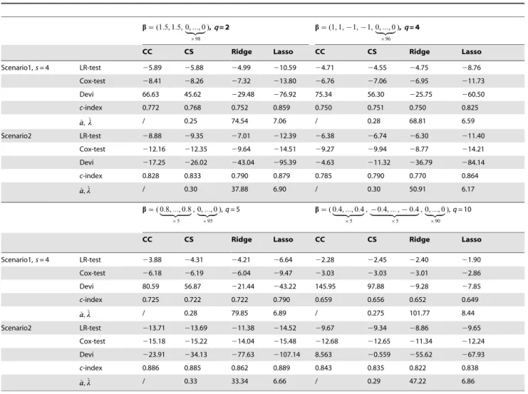
The results for the sparse cases (q= 2, 4, 5 or 10) are given in Table 1. The Lasso generally works best in all prediction measures. This pattern is only violated for the relatively large number of significant covariates (q= 10) where the compound covariate or compound shrinkage method achieves better perfor-mance in terms of the LR-test, Cox-test and c-index. Ridge regression usually performs worst in terms of the LR-test, Cox-test, and c-index. The compound shrinkage method is quite compa-rable in the LR-test, Cox-test, and c-index to the compound covariate method in all cases.

The four methods: CC = compound covariate, CS = compound shrinkage,Ridge = ridge regression, andLasso = Lasso analyses are compared. The median values among the 50 replications for the LR-test (log10P-value), Cox-test (log10P-value),

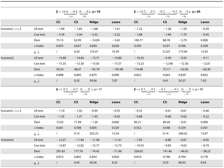
Devi,c-index, and tuning parameters ^aaor^llare reported. The results for the less sparse cases (q= 10, 15, 20 or 30) are given in Table 2. Unlike the sparse cases, the Lasso usually performs worst in terms of the LR-test, Cox-test, and c-index, especially in scenario 1 where the Lasso estimates often result in the null model that has no prediction power (Devi = 0.000, c-index = 0.501,0.538). Overall, the comparative performance of

the compound covariate, compound shrinkage, and ridge regres-sion methods are similar, but in scenario 2, the compound covariate and compound shrinkage methods perform better than the Lasso and ridge regression methods.

The four methods: CC = compound covariate, CS = compound shrinkage,Ridge = ridge regression, andLasso = Lasso analyses are compared. The median values among the 50 replications for the LR-test (log10P-value), Cox-test (log10P-value),

performance in the Devi is not carried over to other measures based on association between the prognostic index and the survival time, i.e., the LR-test, Cox-test, andc-index.

To see the robustness of the proposed method to the cross-validation scheme, we perform the same set of simulations using

K~10cross-validation in place ofK~5. The results (not shown) are virtually identical to these in Tables 1 and 2. Hence, the performance of the compound shrinkage method is less affected by the number of folds used in the cross-validation.

Although we found no single best method across all cases, the comparative performance of the compound covariate and compound shrinkage methods with other methods is remarkable. Unlike ridge and Lasso analyses that may exhibit poor perfor-mance in certain specific cases, the compound covariate and compound shrinkage methods provide more stable performance across different settings with sparse/non-sparse, independent/ correlated informative genes. This robustness property is desirable in practical applications.

We perform similar simulations by increasing the magnitude of non-zero coefficients. As reported in tables S1–5 and S1–6 in Supporting Information S1, prediction performance improved for all four methods, but the relative performances among them are similar to those seen in Tables 1 and 2.

The Primary Biliary Cirrhosis Data Analysis

The primary biliary cirrhosis (PBC) data used in Tibshirani [10] contains 276 patients with 17 covariates. Among them, 111 patients died while others were censored. The covariates consist of a treatment indicator, age, sex, 5 categorical variables (ascites, hepatomegaly, spider, edema, and stage of disease) and 9 continuous variables (bilirubin, cholesterol, albumin, urine copper, alkarine, SGOT, triglycerides, platelet count, and prothrombine). We use log-transformed continuous covariates to get stable results. We compare the prediction performance over 50 random 2:1 splits with 184 patients in the training set and 92 patients in the testing set.

Table 3 reports the results for comparing the compound covariate, compound shrinkage, multivariate Cox regression, ridge regression and Lasso analyses. Multivariate Cox regression analysis exhibits the worst performance, possibly due to a large number of covariates. The other four methods that adapt to high-dimensionality exhibit higher prediction power. Of these methods, the compound covariate method performs best in terms of the LR-test, Cox-test and c-index. This implies that the compound covariate has the highest ability to discriminate between the poor and good prognostic patients in the testing set. Notice that the

Table 1.Simulation results under sparse cases withp= 100 andn= 100 based on 50 replications.

b~(1:5, 1:5, 0,:::, 0

|fflfflffl{zfflfflffl}

|98

),q= 2 b~(1, 1,{1,{1, 0,:::, 0

|fflfflffl{zfflfflffl}

|96

),q= 4

CC CS Ridge Lasso CC CS Ridge Lasso

Scenario1,s= 4 LR-test 25.89 25.88 24.99 210.59 24.71 24.55 24.75 28.76

Cox-test 28.41 28.26 27.32 213.80 26.76 27.06 26.95 211.73

Devi 66.63 45.62 229.48 276.92 75.34 56.30 225.75 260.50

c-index 0.772 0.768 0.752 0.859 0.750 0.751 0.750 0.825

^ a

a,^_ll / 0.25 74.54 7.06 / 0.28 68.81 6.59

Scenario2 LR-test 28.88 29.35 27.01 212.39 26.38 26.74 26.30 211.40

Cox-test 212.16 212.35 29.64 214.51 29.27 29.94 28.77 214.21

Devi 217.25 226.02 243.04 295.39 24.63 211.32 236.79 284.14

c-index 0.828 0.833 0.790 0.879 0.785 0.790 0.770 0.864

^ a

a,^ll / 0.30 37.88 6.90 / 0.30 50.91 6.17

b~( 0:8,:::, 0:8

|fflfflfflfflfflffl{zfflfflfflfflfflffl}

|5

, 0,:::, 0

|fflfflffl{zfflfflffl}

|95

),q= 5 b~( 0:4,:::, 0:4

|fflfflfflfflfflffl{zfflfflfflfflfflffl}

|5

,{0:4,:::,{0:4

|fflfflfflfflfflfflfflfflfflfflfflffl{zfflfflfflfflfflfflfflfflfflfflfflffl}

|5

, 0,:::, 0

|fflfflffl{zfflfflffl}

|90

),q= 10

CC CS Ridge Lasso CC CS Ridge Lasso

Scenario1,s= 4 LR-test 23.88 24.31 24.21 26.64 22.28 22.45 22.40 21.90

Cox-test 26.18 26.19 26.04 29.47 23.03 23.03 23.01 22.86

Devi 80.59 56.87 221.44 243.22 145.95 97.88 29.28 27.85

c-index 0.725 0.722 0.722 0.790 0.659 0.656 0.652 0.649

^ a

a,^ll / 0.28 79.85 6.89 / 0.275 101.77 8.44

Scenario2 LR-test 213.71 213.69 211.38 214.52 29.67 29.34 28.86 29.65

Cox-test 215.18 215.22 214.04 215.48 212.68 212.65 211.34 212.24

Devi 223.91 234.13 277.63 2107.14 8.563 20.559 255.62 267.93

c-index 0.886 0.885 0.862 0.889 0.843 0.835 0.822 0.838

^ a

a,^_ll / 0.33 33.34 6.66 / 0.29 47.22 6.86

NOTE: For Scenario 1, each informative covariate is correlated withsnon-informative covariates. For Scenario 2, the covariates for the right panel have two gene

pathways and those for the left panel have one gene pathway. In each setting,qis the number of informative covariates (covariates with non-zero coefficients).

poor Devi value of the compound covariate method does not affect its prediction power for patients’ prognosis.

NOTE: The median among the 50 replications for the LR-test (log10 P-value), Cox-test (log10 P-value), Deviance, c-index, and

tuning parameters^aaor^llare reported. Smaller values of the LR-test, Cox-test and Deviance, and larger values of the c-index correspond to more accurate prediction performance.

The five methods: CC = compound covariate, CS = compound shrinkage,MultiCox = multivariate Cox regression,

Ridge = ridge regression, and Lasso = Lasso analyses are compared.

The Lung Cancer Data Analysis

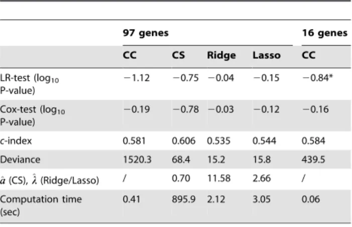
The non-small-cell lung cancer data of Chen et al. [6] is available from http://www.ncbi.nlm.nih.gov/projects/geo/, with accession number GSE4882. The data contains 672 gene profiles for 125 lung cancer patients. Among them, 38 patients died while others were censored. We use a subset consisting of 485 genes whose coefficient of variation in expression values is greater than 3%. We divide the patients into 63:62 training/test datasets as in Chen et al. [6]. Univariate Cox regression analysis based on the training set identifies 16 genes that are significantly related to survival (P-value,0.05). Chen et al. [6] used the 16 regression coefficients to classify the patients of the test dataset into good or poor status. This 16-gene method is a compound covariate analysis applied to the selected set of genes, though the compound covariate method is applicable for the full sets of 485 genes. To illustrate the compound covariate and the compound shrinkage methods with high-dimensional covariates, we selectp= 97 genes whose P-values of the univariate analysis are less than 0.20 in the training dataset of n= 63, and set the coefficients of remaining genes to zero.

Table 2.Simulation results under less sparse cases withp= 100 andn= 100 based on 50 replications.

b~( 0:4,:::, 0:4

|fflfflfflfflfflffl{zfflfflfflfflfflffl}

|10

, 0,:::, 0

|fflfflffl{zfflfflffl}

|90

),q= 10 b~( 0:2,:::, 0:2

|fflfflfflfflfflffl{zfflfflfflfflfflffl}

|10

,{0:2,:::,{0:2

|fflfflfflfflfflfflfflfflfflfflffl{zfflfflfflfflfflfflfflfflfflfflffl}

|10

, 0,:::, 0

|fflfflffl{zfflfflffl}

|80

),q= 20

CC CS Ridge Lasso CC CS Ridge Lasso

Scenario1,s= 2 LR-test 21.99 21.83 21.88 21.41 21.22 21.28 21.29 20.39

Cox-test 23.34 23.34 23.32 22.22 21.68 21.69 21.70 20.45

Devi 75.15 62.99 210.09 25.65 100.77 88.78 23.79 0.000

c-index 0.655 0.657 0.659 0.628 0.595 0.591 0.596 0.538

^ a

a,^_ll / 0.20 125.01 10.39 / 0.225 173.64 12.03

Scenario2 LR-test 215.80 214.84 213.71 214.80 210.35 29.49 29.33 29.11

Cox-test 215.35 215.30 215.05 215.57 213.23 212.98 212.30 212.01

Devi 59.54 48.07 292.79 2103.80 114.48 75.17 263.92 260.30

c-index 0.898 0.895 0.875 0.890 0.852 0.843 0.839 0.832

^ a

a,^ll / 0.35 39.56 7.07 / 0.41 53.37 7.42

b~( 0:2,:::, 0:2

|fflfflfflfflfflfflffl{zfflfflfflfflfflfflffl}

|15

, 0,:::, 0

|fflfflffl{zfflfflffl}

|85

),q= 15 b~( 0:1,:::, 0:1

|fflfflfflfflfflfflffl{zfflfflfflfflfflfflffl}

|15

,{0:1,:::,{0:1

|fflfflfflfflfflfflfflfflfflfflfflffl{zfflfflfflfflfflfflfflfflfflfflfflffl}

|15

, 0,:::, 0

|fflfflffl{zfflfflffl}

|70

),q= 30

CC CS Ridge Lasso CC CS Ridge Lasso

Scenario1,s= 2 LR-test 21.10 21.02 20.95 20.55 20.55 20.61 20.61 20.40

Cox-test 21.35 21.27 21.43 20.42 20.68 20.66 20.62 20.22

Devi 73.02 71.99 21.20 0.000 96.21 89.26 20.01 0.000

c-index 0.601 0.598 0.605 0.529 0.552 0.548 0.559 0.501

^ a

a,^ll / 0.15 263.23 12.54 / 0.14 346.62 13.07

Scenario2 LR-test 212.27 211.84 211.40 211.41 27.93 26.80 26.67 26.05

Cox-test 212.87 212.82 212.77 212.73 210.55 29.83 29.65 28.79

Devi 291.82 177.76 274.42 271.46 326.63 141.46 246.02 238.22

c-index 0.873 0.865 0.854 0.850 0.810 0.790 0.794 0.778

^ a

a,^_ll / 0.45 60.36 8.33 / 0.53 84.43 8.42

NOTE: For Scenario 1, each informative covariate is correlated withsnon-informative covariates. For Scenario 2, the covariates for the right panel have two gene

pathways and those for the left panel have one gene pathway. In each setting,qis the number of informative covariates (covariates with non-zero coefficients).

doi:10.1371/journal.pone.0047627.t002

Table 3.Performance of the five methods based on the primary biliary cirrhosis of the liver data.

CC CS MultiCox Ridge Lasso

LR-test (log10P-value) 27.95 27.00 26.35 26.98 27.11

Cox-test (log10P-value) 212.49211.18 210.71 210.89 210.71

c-index 0.846 0.829 0.825 0.843 0.834

Deviance 101.8 239.9 239.2 249.4 245.9

^ a

a(CS),^_{ll(Ridge/Lasso)} / 0.875 / 22.75 7.32

We compare the compound covariate, compound shrinkage, ridge regression, and Lasso methods as well as the 16-gene compound covariate method of Chen et al. [6]. The results are summarized in Table 4. In terms of the LR-test, the compound covariate method performs best, while, in terms of the Cox-test and c-index, the compound shrinkage method performs best. Figure 2 shows that the two survival curves for the good and poor prognosis groups are best separated by the compound covariate method. However, Figure 3 shows that the Kaplan-Meier curves for the good, medium and poor prognosis groups cross one another and are less distinguishable by the compound covariate method. Here the good, medium, and poor groups are determined by the tertiles of the PI’s in the test datasets. On the other hand, the three Kaplan-Meier curves are well-distinguished in the compound shrinkage method, as implied by its best performance in the Cox-test and c-index (Figure 3; Table 4). This analysis suggests that, compared to the compound covariate method, the compound shrinkage method may provide more accurate ranking of patients’ risks with respect to their survival status. Although ridge regression and Lasso has much smaller deviance, it has poorer performance in the LR-test, Cox-test andc-index.

To see the robustness of the conclusion, comparison of the methods is made under various different numbers of genes, includingp~124genes whose P-values of the univariate analysis are less than 0.25. As seen from the Supporting Information S2, the compound covariate method still performs best in terms of the LR-test. However, the compound shrinkage method still has the best performance in the Cox-test andc-index, and it provides the best separation among the survival curves for the good, medium, and poor prognosis groups. In fact, the compound shrinkage method almost always has the best c-index values under varying number of genes passing a univariate pre-filter for inclusion in the PI (Figure 4). Hence, the conclusion is unchanged.

We also compared the computation time of the four methods in Table 4. The compound covariate method achieves the fastest computation time since it merely repeats p= 97 univariate Cox

regressions using the R ‘‘coxph’’ routine. Ridge regression requires about 5 times and Lasso has about 7 times longer computation time than the compound covariate method. The compound shrinkage is decidedly the slowest, due to the cost of finding high-dimensional maximabb^(^aa)andb^b₍{k)(a).

Analytical Results

Large Sample Results for the Shrinkage Method

The first analytical result of the compound shrinkage method is the large sample consistency of the survival prediction. That is, as

n??with fixedp, the estimated shrinkage parameter^aatends to 1 and the compound shrinkage estimator ^bb(^aa) tends to the true parameter valueb₀. The second and more practically important result is a formula for the standard deviation of^bb(^aa)that may be useful for calculating P-values for each covariate.

To describe the analytical properties of^aaand ^bb(^aa), define, for

k~0, 1, 2,

S(k)(b; t)~X n

i~1

Yi(t)xkiexp (b’xi),s(k)(b; t)~EfS(k)(b; t)=ng,

where x0

i:1, x1i:xi, x2i:xix’i and Yi(t)~I(ti§t) withI(:)

being an indicator function, and forj~1,:::,p,

S(_jk)(b_j; t)~X n

i~1

Yi(t)xkijexp (bjxij),s(jk)(bj;t)~EfS

(k)

j (bj; t)=ng,

E(b; t)~S(1)(b; t)=S(0)(b; t),e(b; t)~s(1)(b;t)=s(0)(b; t),

Ej(bj;t)~S

(1)

j (bj;t)=S

(0)

j (bj;t), ej(bj; t)~s

(1)

j (bj;t)=s

(0)

j (bj; t),

V(b;t)~S(2)(b;t)=S(0)(b; t){E(b; t)E(b; t)’_,

Vj(bj; t)~S

(2)

j (bj;t)=S

(0)

j (bj; t){Ej(bj; t)2:

The score function defined as the derivative of‘a

n(b)with respect

tobis given by

Ua_n(b)~X n

i~1

difxi{aE(b; ti){(1{a)(E1(b1;ti),:::,Ep(bp; ti) )’g:

The observed Fisher information matrix, the negative of the Hessian of‘a

n(b), is

Va_n(b)~X n

i~1

difaV(b; ti)z(1{a)diag(V1(b1; ti),:::,Vp(bp; ti) )g,

where diag(V1(b1; ti),:::,Vp(bp; ti) ) is the diagonal matrix

with the diagonal element(V1(b1; ti),:::,Vp(bp; ti) ). It is easy

to verify that Va_n(b) is positive semi-definite and hence ‘a n(b) is

Table 4.Performance of the five methods based on the non-small-cell lung cancer data of Chen et al. [6].

97 genes 16 genes

CC CS Ridge Lasso CC

LR-test (log10

P-value)

21.12 20.75 20.04 20.15 20.84*

Cox-test (log10

P-value)

20.19 20.78 20.03 20.12 20.16

c-index 0.581 0.606 0.535 0.544 0.584

Deviance 1520.3 68.4 15.2 15.8 439.5

^ a

a(CS),^_{ll(Ridge/Lasso)} / 0.70 11.58 2.66 /

Computation time (sec)

0.41 895.9 2.12 3.05 0.06

NOTE: Smaller values of the LR-test (log10P-value), Cox-test (log10P-value) and

Deviance, and larger values of thec-index correspond to more accurate prediction performance.

*If good and poor groups are separated by the median PI in the training set, the LR-test has P-value = 0.034 (log10P-value =21.47) withn= 28 in the good and

n= 34 in the poor groups (the same result as Figure 1C of Chen et al. [6]).

The methods:CC= compound covariate (using 97 or 16 genes),CS = compound shrinkage,Ridge= ridge regression, andLasso= Lasso analyses are compared.

concave for a given a[½0, 1. For a[½0, 1), Va

n(b) is typically

positive definite and ‘a

n(b) is strictly concave, which implies that

^

b

b(a)is unique even whenpwn.

Now we state the large sample results asn??with fixedp; the proofs are given in Supporting Information S3. Assume that f(ti,di,xi); i~1, . . .,ng are independently and identically

distributed under the model (1) withb~b0, anda[½0, 1is a fixed constant. Applying martingale calculus and the concave property of‘a

n(b)under mild regularity conditions (e.g. p.497–498 of [28]),

we verify that^bb(a)converges in probability tob(a), a solution to a h(a,b)~0for a givena[½0, 1where

h(a,b)~ ð ?

0

s(1)(b₀;u)h0(u)du{

ð ?

0

ea(b;u)s(0)(b₀;u)h0(u)du, ð8Þ

whereea(b; u)~ae(b;u)z(1{a)(e1(b1;u),:::,ep(bp;u) )’:

Note that, fora~0, equation (8) is a multivariate generalization of equation (2–5) of Struthers and Kalbfleish [29] in the context of the misspecified Cox regression analysis. Fora~1, the solution to h(1,b)~0isb₀, and henceb(1)~b₀.

Proposition 1 (Consistency): Asn??,^aaconverges in probability to 1. Also,^bb(^aa)converges in probability tob0.

Proposition 2 (Asymptotic normality): As n??, pffiffiffin(^aa{1 ) converges weakly to a mean zero normal distribution with variance vCV(b0). Also,

ffiffiffi n

p

(^bb(^aa){b₀) converges weakly to a mean zero normal distribution with covariance matrix S(b0). Explicit formulas forvCV(b0)andS(b0)are derived in Supporting Information S3.

Remark I.We allow^aaw1whenCV(a)is maximized ataw1. Remark II.The asymptotic varianceS(b₀)can be consistently estimated byS^aa_n(^bb(^aa) ), where

Figure 2. Kaplan-Meier curves for the 62 patients in the lung cancer data of Chen et al.[6].Good (blue) and poor (red) groups are determined by the median of the PI’s in the test dataset.

Sa_n(b)~Aa_n(b) V

a n(b)

n

{1

Aa_n(b)’_,

Aa_n(b)~V a n(b)

{1_{_} h

hn(b)hh_n(b)’

{d2_CV(a)=da2 zIp,

_

h hn(b)~

LUa_n(b) La

~X

n

i~1

dif{E(b; ti)z(E1(b1;ti),:::,Ep(bp; ti) )0g,

whereIpis the unit matrix of sizep. The estimatorSana^(^bb(^aa) )

gives reasonable approximation to the variance of^bb(^aa)even when

pis large (see simulations forp= 100 andn= 100 in Supporting Information S3). The variance estimate facilitates the Wald-type test for significance of the regression coefficients.

Analytical Comparison with the Lasso and Ridge Regression

Unlike the Lasso and ridge regression in equations (3) and (4), which shrink the regression coefficients toward0~( 0,:::, 0 )’_{, the} compound shrinkage estimator is obtained by shrinking the coefficients toward the compound covariate estimator ^

b

b(0)~(^bb₁(0),:::,^bb_p(0) )’_.

We apply a statistical large sample theory on the misspecified Cox regression analysis [29,30] to demonstrate that shrinking the regression coefficients toward the compound covariate estimator may be more informative than shrinking toward0when covariates are independent. Whenngoes to infinity, the compound covariate estimator ^bb(0) converges in probability to a vector

b(0)~(b₁(0),:::,b_p(0) )’, a solution toh(0,b)~0that is defined in equation (8). In general,b(0)=b₀, whereb₀~(b₀₁,:::,b_0p)’_is the true parameter value in equation (1). Nevertheless, b(0) contains information aboutb₀. Without loss of generality, we will describe the properties of the first componentb₁(0)ofb(0), where

Figure 3. Kaplan-Meier curves for the 62 patients in the lung cancer data of Chen et al.[6].Good (blue), medium (black), and poor (red) groups are determined by the tertile of the PI’s in the test dataset.

the censoring is assumed independent of survival time and covariates.

(P1) Ifb₀₂~ ~b_0p~₀, thenb₁(0)~b₀₁.

(P2) Suppose thatxi1and(xi2,:::,xip) are independent for all i(~1, . . .,n). If b₀₁~0, then b₁(0)~0. If b₀₁=0, then 0vb₁(0)vb₀₁when0vb₀₁, orb₀₁vb₁(0)v0whenb₀₁v0.

The property (P1) is due to the fact that the univariate Cox estimate^bb₁(0)is obtained under the assumption that the hazard given xi1 is of the form h01(t) exp (b1xi1), which is true when b₀₂~ ~b_0p~0under equation (1). An important implication from the property (P1) is that, ifb₀~0, thenb(0)~0as well. The property (P2) is deduced from some known results of misspecified Cox regression analysis [29,30]. The property (P2) implies that, if all the covariates are independent, the sign of each component of

b(0)agrees with that ofb₀, andb(0)is closer tob₀than0. From the above properties, it is then expected that shrinking the regression coefficients towardb(0)may be more informative than shrinking them toward0. This gives an analytical reason justifying the proposed shrinkage method. The justification in the presence of correlations among covariates is analytically intractable, and hence is done by simulations and real data analysis as presented above.

The proposed shrinkage method has a natural interpretation under a setting of linear regression. Lety~(y1,:::,yn)’be the

response vector andX’~(x1,:::,xn)be the design matrix, where xi~(xi1,:::,xip)’is the covariate for individuali. In the ordinary

least square regression, we minimize the objective function

Pn

i~1(yi{b’xi)2. Ifpwn, it does not have a unique minimizer

since the design matrixX’Xis singular. The proposed shrinkage scheme leads to minimizing.

aX

n

i~1

(yi{b’xi)2z(1{a)

Xn

i~1

Xp

j~1

(yi{bjxij)2,

for some a[½0, 1). The minimizer of the above function is unique and written as

^

b

bShrink(a)~½aX’Xz(1{a)diag(X’X){1 X’y

wherediag(X’X) is a diagonal matrix with the same diagonal elements as in X’X. The singularity of X’X is thus resolved by reducing the off-diagonal values by amultiplicativefactora. This is in contrast to ridge regression [13] where the diagonal values are increased by anadditivefactorlw₀, that is,

^

b

bRidge(l)~½X’XzlIp {1

X’y:

Figure 4. Thec-index assessments of the four methods under varying number of top genes (p= 16,124 ) in the lung cancer data of

Chen et al.[6], where ‘‘top genes’’ refer to most strongly associated genes passing a univariate pre-filter for inclusion in the linear predictor (PI).

With complete shrinkage, the difference between the two estimators becomes evident since^bbShrink(0)~_fdiag(X’X)g{1

X’y while^bbRidge(?)~0.

Computing Algorithms

Numerical maximization of‘a

n(b) in equation (6) can be done

through quasi-Newton type algorithms. For instance, the R ‘‘nlm’’ is a reliable routine to find the minimum of{‘a

n(b)with a largep.

Numerical maximization of CV(a) in equation (7) can be obtained by a grid search on finely selected values of a as commonly done in cross-validation [17,24]. In our numerical studies we observe that the graph of CV(a) is always unimodal, and calculating CV(a)with smaller ais always faster than with larger a. Utilizing these properties, we suggest the following computation algorithm, which is more efficient in computation than the ‘‘exhaustive search’’ procedure:

Step 1:Seta~0and a positive numberDa (e.g., Da~0:025), and calculateCV(0).

Step 2: Set a~az_Da. If a§1, then go to Step 3. If

CV(a₎ƒCV(a), then go to Step 3. If CV(a₎wCV(a), then seta~a_{and return to Step 2.}

Step 3:Stop the algorithm and set^aa~a.

Conclusions

We have revisited a compound covariate prediction method for predicting survival outcomes with a large number of covariates. This method is popularly employed in medical studies, but its statistical performance has been less studied in the literature. We investigate the prediction power of the method by comparison with the well-known methods of ridge regression and Lasso, both of which adapt to a large number of covariates. The simulations demonstrate that the compound covariate method has better predictive power than ridge regression when only a few among a large number of covariates associate with the survival (i.e., sparse cases), and that it performs better than the Lasso when many of a large number of covariates simultaneously affect the survival (i.e., less sparse cases). The compound covariate method exhibits best predictive power among all the competitors in the primary biliary cirrhosis dataset, including the multivariate Cox regression, ridge regression and Lasso. In the even much higher dimensional lung cancer microarray data, where the multivariate Cox regression no longer applies, the compound covariate method similarly outper-forms ridge regression and Lasso. Hence, the compound covariate method is a computationally attractive and powerful technique for survival prediction with a moderate or large number of covariates. To further improve the prediction power of the compound covariate prediction, we propose a novel shrinkage type estimator for survival prediction with a large number of covariates. The new shrinkage scheme refines the compound covariate method by incorporating the multivariate likelihood information into the compound covariate predictor. Our simulation studies demon-strate that, in the sparse signal setting, the Lasso strongly outperforms the ‘‘non-sparse’’ methods, including ridge regression, compound covariate and compound shrinkage methods. On the other hand, in settings with less sparse signals, the compound covariate and compound shrinkage methods perform comparably to ridge regression, and all these methods outperform the Lasso method. Given that the non-sparse setting is not uncommon [27], and ridge regression shows best overall performance in several comparative prediction studies [17,18,19], the compound covar-iate and compound shrinkage methods have the potential to be useful alternatives. Our proposal also provides a novel framework

of shrinkage estimation that encompasses the simple but effective compound covariate method as a special case. In the lung cancer data analysis we find that, the major advantage of the proposed compound shrinkage method over the compound covariate method is in its more accurate prediction of patient’s survival status. We also establish statistical large sample theories, including consistency and standard error estimation of the parameter estimator, for the proposed shrinkage method. Given these numerical and theoretical evidences, the proposed prediction scheme seems to be a method that can be reliably applied for survival prediction. The method is implemented by an R package ‘‘compound.Cox’’ available in CRAN at http://cran.r-project. org/.

A potential extension of the proposed shrinkage method is the development of covariate selection. This is clearly an important issue in microarrays in which the focus is to select genes that achieve good predictive power. If the gene selection is the main focus, we find the Lasso method offers an elegant solution since it gives an automatic way of selecting genes. In fact, the Lasso shows excellent performance when the signal is sparse, as shown in our simulation studies (Table 1). However, in the presence of a large number of informative genes (less sparse cases), the performance of the Lasso is less reliable since it tends to select only a few genes among them and often results in the null model with no prediction power (Table 2). A large number of informative genes are also encountered in the lymphoma data reported in Matsui [16], where the number of genes in the optimal set ist= 75 or 85. Matusi [16] suggests agene filteringprocedure that chooses the top tgenes in terms of univariate Cox analyses, where tis the threshold that leads to the best predictive power in cross validation. Although this methodology is computationally simple, the toptgenes are based on univariate significance only. Hence, it is interesting to extend the gene filtering approach to take into account the combined, multivariate predictive information of genes using the proposed shrinkage method. We will leave this problem to a future research topic.

Supporting Information

Supporting Information S1 Simulation results forp= 50

and 200 (tables S1–1 , S1–4) and for the increased magnitudes of the regression coefficients (tables S1–5, S1–6).

(PDF)

Supporting Information S2 Comparison of the predic-tion methods for the lung cancer data withp= 124 genes. (PDF)

Supporting Information S3 Proofs of Propositions 1 and 2, variance estimation, and simulation results for variance estimation.

(PDF)

Acknowledgments

The authors would like to thank the academic editor and the two referees for their helpful comments that greatly improve the paper.

Author Contributions

References

1. Jenssen TK, Kuo WP, Stokke T, Hovig E (2002) Association between gene expressions in breast cancer and patient survival. Human Genetics 111: 411– 420.

2. van de Vijver MJ, He YD, van’t Veer LJ, Dai H, Hart AAM, et al. (2002) A gene-expression signature as a predictor of survival in breast cancer. N. Eng. J. Med 347: 1999–2009.

3. van’t Veer LJ, Dai H, van de Vijver MJ, He YD, Hart AA, et al. (2002) Gene expression profile predicts clinical outcome of breast cancer. Nature 415: 530– 536.

4. Zhao X, Rodland EA, Sorlie T, Naume B, Langerod A, et al. (2011) Combining gene signatures improves prediction of breast cancer survival. PloS ONE 6(3): e17845.

5. Beer DG, Kardia SLR, Huang CC, Giordano TJ, Levin AM, et al. (2002) Gene-expression profiles predict survival of patients with lung adenocarcinoma. Nature Medicine 8: 816–824.

6. Chen HY, Yu SL, Chen CH, Chang GC, Chen CY, et al. (2007) A five-gene signature and clinical outcome in non-small-cell lung cancer. N Engl J Med 356: 11–20.

7. Shedden K, Taylor JMG, Enkemann SA, Tsao MS, Yeatman TJ, et al. (2008) Gene expression-based survival prediction in lung adenocarcinoma: a multi-site, blinded validation study. Nature Medicine 14: 822–827.

8. Cox DR (1972) Regression models and life-tables (with discussion). Journal of the Royal Statistical Society, Series B 34: 187–220.

9. Brazma A, Culhane AC (2005) Algorithms for gene expression analysis. In: Dunn JM, Jorde LB, Little PFR, Subramaniam S, editors. Encyclopedia of Genetis, Genomics, Proteomics and Bioinformatics. London: John Wiley and Sons.

10. Tibshirani R (1997) The lasso method for variable selection in the Cox model. Stat. in Med. 16: 385–395.

11. Gui J, Li H (2005) Penalized Cox regression analysis in the high-dimensional and low-sample size settings, with applications to microarray gene expression data. Bioinformatics 21: 3001–3008.

12. Segal M (2006) Microarray gene expression data with linked survival phenotypes: diffuse large B-cell lymphoma revised. Biostatistics 7: 268–285. 13. Hoerl AE, Kennard RW (1970) Ridge regression: biased estimation for

nonorthogonal problems. Technometrics 12: 55–67.

14. Verveij PJM, van Houwelingen HC (1994) Penalized likelihood in Cox regression. Stat. in Med. 13: 2427–2436.

15. Radmacher MD, Mcshane LM, Simon R (2002) A paradigm for class prediction using gene expression profiles. Journal of Computational Biology 9: 505–511. 16. Matsui S (2006) Predicting survival outcomes using subsets of significant genes in

prognostic marker studies with microarrays. BMC Bioinformatics 7: 156. 17. Bovelstad HM, Nygard S, Storvold HL, Aldrin M., Borgan O, et al. (2007)

Predicting survival from microarray data – a comparative study. Bioinformatics 23: 2080–2087.

18. van Wieringen WN, Kun D, Hampel R, Boulesteix AL (2009) Survival prediction using gene expression data: A review and comparison. Comp. Stat. & Data Anal. 53, 1590–1603.

19. Bovelstad HM, Borgan O (2011) Assessment of evaluation criteria for survival prediction from genomic data. Biometrical Journal 53: 202–216.

20. Verveij PJM, van Houwelingen HC (1993) Crossvalidation in survival analysis. Stat. in Med. 12: 2305–2314.

21. Goeman JJ (2010) L1 penalized estimation in the Cox proportional hazards model. Biometrical Journal 52: 70–84.

22. Witten DM, Tibshirani R (2010) Survival analysis with high-dimensional covariates. Stat. Meth. in Med. Res. 19: 29–51.

23. Tukey JW (1993) Tightening the clinical trial. Controlled Clinical Trials 14: 266–285.

24. Tibshirani R (2009) Univariate shrinkage in the Cox model for high dimensional data. Statistical Applications in Genetics and Molecular Biology 8: 1–21. 25. Harrell FE, Califf RM, Pryor DB, Lee KL, Rosati RA (1982) Evaluating the

yield of medical tests. Journal of the American Medical Association 247: 2543– 2546.

26. Harrell FE, Lee KL, Mark DB (1996) Multivariate prognostic models: issues in developing models, evaluating assumptions and adequacy, and measuring and reducing errors. Stat. in Med. 15: 361–387.

27. Kraft P, Hunter DJ (2009) Genetic risk prediction–Are we there yet? N Engl J Med 360: 1701–1703.

28. Andersen PK, Borgan O, Gill RD, Keiding N (1993) Statistical Models Based on Counting Processes. New York: Springer-Verlag.

29. Struthers CA, Kalbfleish JD (1986) Misspecified proportional hazard models. Biometrika 73: 363–369.