doi: 10.1590/0101-7438.2016.036.01.0045
ANALYSIS OF SHIP ARRIVAL FUNCTIONS IN DISCRETE EVENT SIMULATION MODELS OF AN IRON ORE EXPORT TERMINAL
Romeu Rodrigues
1and Jo˜ao Jos´e de Assis Rangel
2*Received November 11, 2014 / Accepted February 29, 2016
ABSTRACT.This work evaluates the results of different distribution functions of ships arrivals in the sim-ulation of an iron ore export terminal under implementation. The system adopted for the analysis applied a real case designed for installation of a Brazilian company terminal. The analysis was carried out by a discrete event simulation model. Variations of up to 566% in predicting demurrage paid to ships are de-tected. A database with 2,518 arrivals of ships demonstrates that, unlike recommendations of the traditional literature, the Pearson 6 function is the one that better represents the distribution to a shipping terminal of iron ore than the Exponential, Erlang and Weibull functions.
Keywords: computer simulation, port, demurrage, ship-berth link, probability distributions.
1 INTRODUCTION
The motivation to explore the theme of iron ore shipments at port terminals comes from the fact that Brazilian exports have added nearly US$200 billion in 2008 (Fleury & Hijjar, 2008) and US$256 billion in 2011 (Webber, 2012), and the export of iron ore, a significant stake in the country’s trade balance in recent years: US$42 billion in 2011 and US$31 billion in 2012. That highlights the importance of further investigations, given that the literature has empha-sized the study of container ports. For researching articles related to Science Direct database (www.sciencedirect.com/science), in 2005-2014, using the keyword berth allocation, 33 refer-ences to container terminals were found among the topics outlined, and no one about iron ore terminals.
In general, the performance analysis in port terminals has been a theme of interest for several researchers as Dragovic et al. (2005). Yin et al. (2011) pointed out that studies on control oper-ations of ships arrivals are important to help reduce costs for shipping terminals and to motivate more detailed investigations on the subject. Those investigations highlighted the importance of the interconnection between the operations of receiving, storage and delivery of loads. Many of
*Corresponding author.
1R Rodrigues Consultoria, Linhares, ES, Brasil. E-mail: [email protected]
them indicated the use of computer simulation as a tool to maximize the use of facilities and minimize investments in operational improvements as in the works of Casaca (2005), Parola & Sciomachen (2005), and Canonaco et al. (2008).
For analysis applying computer simulations, it is necessary to select parameters for data input and choose the method by which the results will be evaluated. Camelo et al. (2010) simulated the operation of a new berth of a marine terminal in the northeastern of Brazil from input data of another similar berth of the same terminal. They adopted the Exponential function to generate the arrival times of ships. Wanke (2011) also adopted Exponential functions for the ships arrival. His study determined the parameters of these Exponential functions from real data of a container terminal in the Brazilian southeastern. In another work, Demirci (2003) mentioned that the func-tions generally recommended in the literature for arrival of ships are the Exponential, Weibull and Erlang.
However, when it comes to simulate a completely new terminal in project (“green field” project in business language), it increases the difficulty in carrying out the analysis of those relationships. Ignacio & Neves (2009) approached the problem by showing the importance of the parameters to be adopted in the model. They referred to the use of the Poisson function distribution for the arrival of ships but not making explicit their parameters. Incidentally, this is the great difficulty encountered by modelers to “green field” designs: the lack of clear explanation of the parameters of the functions adopted.
In assessing the results, the main variables for evaluating the operability of a port terminal con-sidered by their managers are the demurrage, the average queue, the occupancy rate of berth and the lead time – time between the beginning and the end of some activity (Kim et al., 2003). The demurrage is the amount paid by the port to the ship by waiting beyond an agreed term (Nishimura et al., 2001). The total cost of demurrage, besides measuring the operational effi-ciency of the port terminal, is used by managers to make decisions about purchasing equipment and investments in operational improvements (Legato & Mazza, 2001).
When returning to the issue about the input functions in the simulations, it could be seen that several studies have indicated that the ship arrivals in the terminals have been increasingly con-trolled and less random, even as a result of the adoption, by the terminals, of adherent policies to the results of the own simulations. According to Wanke (2011), the costs of demurrage can be reduced if rules of different priorities of the FIFO (first in first out) may be adopted. In accor-dance to the author, the best combination of pier allocation policy and of priority for mooring is the one that implies the lowest total cost of demurrage. The impact of the arrival processes of ships on the results of the simulations tends to be underestimated. He concluded that the waiting times of ships are significantly affected by the type of premise of their arrival, whether or not controlled. Among three distributions studied, the Poisson showed to be the worst result, while the distribution of arrival managed through the inventory control was the one that brought better results for a liquid bulk terminal that receives and distributes chemical products.
The aim is to demonstrate that the input functions recommended in the literature, especially the Exponential, Erlang and Weibull, used in simulations of shipment of iron ore in port terminals, design very different results, which may lead to bad decisions and oversizing of investments. The simulation explored a database with 2,518 consecutive ships arrivals at a terminal similar to the green field under study to demonstrate that a Pearson 6 function is the proper function to simulate a ship arrival related to the reality of this type of terminal. Moreover, the research draws attention to the need of simulation studies that define the parameters of the input functions.
This article is divided as follows: In the Introduction (Item 1), the motivation was made explicit, its general bases with brief literature review were exposed and presented the aim; in the next section (Item 2 – Objectives and Background), the main aspects are defined in more details, pre-senting major questions to be answered; Item 3 – Methodology, the physical system, simulation and conceptual models and configuration of the experiments as well as the evaluation method are described. Finally, after discussion of results (Item 4), the conclusions (Item 5) are presented.
2 OBJECTIVE AND BACKGROUND
This section exposes in detail the research questions and the objectives. Besides, it explains some concepts approached in this study and the main works found in the literature review.
2.1 Issues to be answered
1. How significant are the input functions in the simulation?
2. What level of impact does the choice of different functions have in the results?
3. To what kind of decision do the results lead?
4. In what can literature contribute for the calibration of simulations of “green field” projects?
2.2 Objectives
As discussed in the introduction, the aim of this study is to investigate the importance and the impact of the choice of input functions on the results of the simulated models. In this case, the function that should represent the arrival of ships to be attended at a port terminal is applied for this investigation. Three types of functions are compared with one taken from a database of a terminal similar in size and capacity. The intent is to demonstrate that the results can lead to different decisions in terms of investment. They may even unnecessarily raise the prices of a project at a conceptual stage.
2.3 Demurrage
as the amount paid by the port to the ship for waiting beyond a deadline agreed. When the port is contracted to receive and load a particular ship, a period called lay days, within which the ship shall be moored and loaded, is established. If the port, for its responsibility, is unable to load the ship within that time limit, it must pay the daily cost of the ship, once that deadline runs out. Unlike the demurrage, there is the dispatch that is the reward received by the port when it advances the operation of the ship, releasing it before the agreed time limit.
In the present work, the demurrage is calculated as follows: After the NOR-Notice of Readiness of the ship (notice of arrival in the queue), the port has 60 hours to moor it, ship the ore and deliver the documents. The cost of demurrage is estimated at US$18,000/day for Capesize and US$10,000/day for Panamax. According to Alizadeh & Talley (2011), the Panamax size ships are from 60,000 to 80,000 dwt, and the Capesize, more than 80,000 dwt, normally 120,000 to 180,000 dwt (where dwt: deadweight). The dispatch will have value of 50% of demurrage. Example: If a Capesize ship between the NOR and the release of berth takes 62 hours, there will be demurrage equal to US$1,500.00. It is showed in Equation 1:
Period of Time = 62−60=2h
Demurrage= 2h{Period of Time}
24h ∗US$18,000.00 = US$1,500.00
(1)
If, on the other hand, it takes 50 hours, there will be a dispatch equal to US$3,750.00, showed in Equation 2:
Period of Time = 60−50=10h
Demurrage=10h{Period of Time}
24h ∗US$18,000.00∗50% = US$3,750.00
(2)
2.4 Some probability distributions applied on simulation
A very brief look at probability distributions shows that the Exponential distribution is one of the most used in simulation models. However, it has a large variability. The main use is in the modeling of periods between two events such as time between arrivals entities in a system, time between failures or customer service time (Banks et al., 2010 and Law, 2007).
Erlang distribution is used in the simulation of certain types of processes, often in situations in which an entity enters a station to be serviced sequentially through a series of stations.
The Weibull distribution is extensively used in models that represent the equipment lifetime.
Beta distribution, due to its ability to adapt itself to various forms, is used as an approximation, when there is no data available.
The Pearson 6 distribution is used similar to those situations where it is used to Exponential and sometimes the Erlang.
Other statistic distributions as Triangular, Normal and Exponential were indicated by Chwif & Medina (2010) as more usual in these kind of processes.
2.5 Related Works
Casaca (2005) stated that a container terminal is an intermodal node to where different modes of transport converge. She also divided port operations into three systems: ship, internal processing and road. Those can be generalized to any port terminal because, at exporters and importers terminals, general cargo and liquid or solid bulk can be received and shipped by pipeline, trucks or ships and boats.
Tu & Chang (2006) considered that those transactions in container yards directly affect the op-erations of ships. This can also be extended to solid bulk terminals, since the recovery machines expend time to move from a pile to another and belt conveyors have lack of time to change lanes.
Parola & Sciomachen (2005) evaluated the effects of different percentages of road and rail modes in the terminal entrance due to the growth of ships demand.
Demirci (2003) examined the bottlenecks of a port system and proved that simulation is very useful to minimize investment to remove operational bottlenecks.
Dragovic et al. (2005) analyzed effects of efficiency and accuracy over ships attendance times when priorities are admitted to some classes of ships through simulation model in a container terminal.
Duinkerken et al. (2007) compared the impact of different containers transport systems at a ter-minal over costs of operations, in order to support investment management decisions.
Ottjes et al. (2007) proposed a generic structure simulation model for container handling and demonstrate the importance of transport flows, transfer and storage over the terminal infrastruc-ture.
Kim et al. (2003) propose a dynamic programming model for the sequencing problem of the truck arrival in container port terminals.
Legato & Mazza (2001) showed that simulation is a useful tool to suggest how to improve the capacity of resources and modify the policies of their application that directly affect the perfor-mance offered to shipping companies.
Ho & Ho (2006) indicate that, given that investments in port infrastructure are too high, it is very important that call times of ships in ports be minimized in order to maximize the facilities usage.
According to Nishimura et al. (2001), planning the allocation of ships at berths is a key factor for efficient use of public docks in ports.
Meisel & Bierwirth (2009) investigated the twin problems of allocating both ships at berths as cranes for their attendance in container terminals. Note that the productivity of quay cranes is very important to plan the choice of the berths for each ship.
Yin et al. (2011) proposed a port planning manager system able to generate successful programs as part of berths control module, a transport allocation module and a storage module in the yards for a container terminal.
Liu & Takakuwa (2011) analyzed the processing time and the operations flows bottlenecks using electronic tracking data in real time, concluding that the information obtained through simulation are suitable for performance analysis of the operation.
Simulations of port terminals have, as tips, on the one hand, the arrival of the ships to be loaded and, on the other hand, the possible payment of demurrage by the port due to the waiting time to dock. To perform them, it is generally recommended (Wanke, 2011), to the arrival of ships, exponential functions (Demirci, 2003) (Pachakis & Kiremidjian, 2003); negative exponential (Shabayek & Yeung, 2002); and Weibull (Tahar & Hussain, 2000). For iron ore, it is suggested to Erlang function (UNCTAD, 1985).
Camelo et al. (2010) simulated the operation of a marine terminal considering that arrivals follow Poisson and ships calls follow Erlang distribution.
According to Van Asperen et al. (2003), the impact of the arrival processes ships on the results of the simulations tend to be underestimated. They conclude that waiting times of ships are signifi-cantly affected by the type of premise of their arrival under control or not. Among three functions studied, the Poisson reveals the worst result, while the arrival managed through inventory control brings better results.
Psaraftis & Kontovas (2014) modeled combinations of routes and speed ships aiming to optimize their operating costs. They confirmed that the owners delay or advance their ships traveling in order to reduce the waiting time for mooring, which, again, decreases the randomness of the arrival process.
The brief review above shows few studies about bulk cargo terminals. The references about this kind of port terminal can be reached only in Camelo et al. (2010), Ignacio & Neves (2009) and Van Asperen et al. (2003). Bugaric & Petrovic (2007), Cassettari et al. (2011), van Vianen et al. (2012), Bugaric et al. (2012) and Cigolini et al. (2013) presented simulation works about terminals in order to optimize load, discharge and transshipment operations, always seeking the best way to reduce ships delays and investments.
Thus, we can conclude that simulation is the best method to treat the operating results of a fore-cast problem of a port terminal. The installation is inserted in the transport context and logistics, operations, procurement and, especially, in production processes. Most of these studies are refer-ent to container terminals, some about liquid bulk cargo and a few of them about dry bulk cargo terminals, especially few about iron ore terminals.
3 METHODOLOGY
This item presents the methodology applied for the design of the simulation model. For this, the physical system is previously described as well as general considerations about iron ore ports. It also shows the conceptual model of the referred system and the configuration for the implementation of the simulated experiments.
3.1 Description of the system
3.1.1 General considerations about iron ore ports
An iron ore terminal generally operates receiving iron ore via trains or ducts. This iron ore is usually transported by conveyor belts from the point of receipt to the storage yard. The product is stored in the yard by large stackers moving on rails. Large piles formed wait for the mooring of ships, when bucket wheel or cylinders recliners, also moving on rails, collect them, sending the material by belt conveyors to the ship loaders, which put them in the hold of the ships.
The rates of movement are, in general, of thousands of tons per hour. Those rates need to be consistent with the ship size so that its freight will be cheaper. Therefore, its cost to remain queued on the port is too high. Thus, one of the most important elements in the port is its ability to ship and, at the end, its ability to quick service to ships, keeping small queues. This creates an imbalance between the capacity of reception and dispatch, because, typically, the reception has a slower pace, but more solid, while the shipment needs to be faster, intermittent.
Sufficient yard areas are also needed to ensure inventory to meet the ships, since each of them, as a rule, takes one or more different types of products.
As for the arrival of ships in port, the central theme of this work, one should bear in mind that it is not completely random as it may seem at first. There are cases, in container terminals, in which shipowners “buy” from the port periodic “windows” (weekly, in general) for mooring of ships of their lines. Thus, these ships do not expect freight and always meet a fixed schedule. This is a case that typically deviates from queueing theory. The control that navigation agencies have on their ships is also great in the port terminals of iron ore. It is common, for example, that the agencies reduce the speed of a ship when it is too early to reach the port. Therefore, it saves fuel and spends less time waiting in line to moor. This brings us to ask what kind of distribution function of arrival of ships may be used in simulations of operational performance of ports.
3.1.2 Description of the physical system
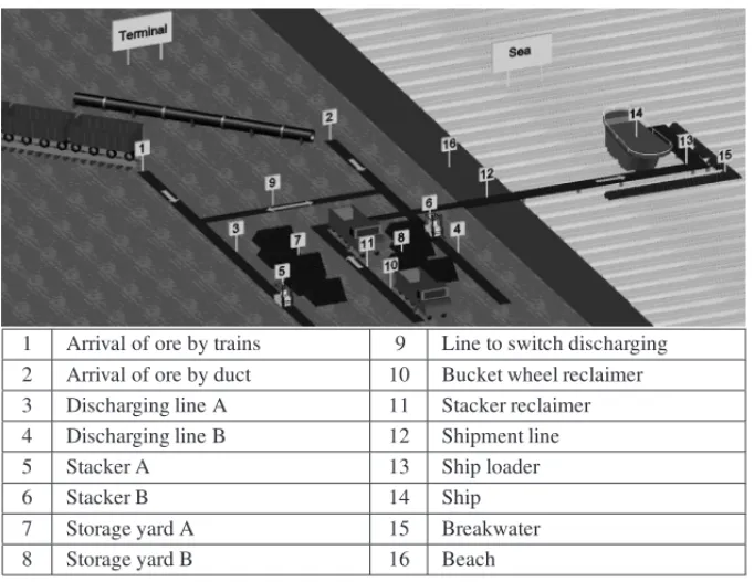
capacity of 2.5 million tons; recovery (operation yard) through a bucket wheel reclaimer and a stacker reclaimer; translation to the ship, again through conveyor belts; and shipment (process called outbound). The general scheme is illustrated in Figure 1.
1 Arrival of ore by trains 9 Line to switch discharging 2 Arrival of ore by duct 10 Bucket wheel reclaimer 3 Discharging line A 11 Stacker reclaimer 4 Discharging line B 12 Shipment line
5 Stacker A 13 Ship loader
6 Stacker B 14 Ship
7 Storage yard A 15 Breakwater
8 Storage yard B 16 Beach
Figure 1– Schematic model of port terminal for ore shipment.
Here, it is considered a port with capacity of total reception via ore pipeline of 6,800 ton/h and via train of 7,000 ton/h. It has been estimated that the trains can feed the system with four different types of products, while the ore pipeline can do it with two types.
In the shipment system, the port has only one entrance, a berth of mooring and a nominal ship-ment capacity of 8,000 ton/h for each of the two bucket wheels and of 16,000 ton/h for the ship loader. Times of operational shutdowns were estimated based on actual operations, such as exchange of train, displacement of stackers for repositioning in the yards and for preventive maintenance and breakage.
The operation time for each ship enter through the navigation channel depends on the extent of access channel and turning basin geometry. In this case, the time of navigation, mooring and release of documents has been estimated between 2.75 and 3.58 hours and dispatch, unmooring and exit, releasing the berth, between 2.33 and 3.33 hours.
Two types of ships were considered, PANAMAX and CAPESIZE, with cargo capacity of 80 and 180 thousand tons respectively.
the stackers (5) and (6), which pile it in the storage yard (7) and (8). There is a line to switch the discharging (9) between the yards so that the ore can go to any of the yard from any entrance.
Once the ship is moored, the ore is taken from the yards by bucket wheel reclaimer (10) or stacker reclaimer (11) and, then, via belt conveyors of the shipment line (12), goes to the ship loader (13), which deposits it in the ship’s hold (14). It stays moored in a berth protected by the breakwater (15).
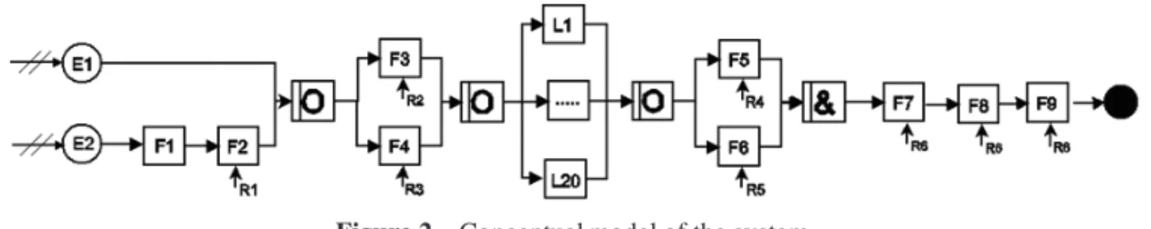
3.2 Simulation Model 3.2.1 Conceptual Model
The simulation model was constructed using the methodology proposed by Banks et al. (2010), with the following specific steps for this work: formulation and analysis of the problem; project planning; formulation of the conceptual model; macro information and data collection; transla-tion of the model; verificatransla-tion and validatransla-tion; experimental project; experimentatransla-tion; interpreta-tion and statistical analysis of the results; and documentainterpreta-tion and presentainterpreta-tion of the results.
The simulations were initiated after the model was completely verified and validated, following the methodology proposed by Sargent (2013). The simulated experiments were conducted based on the methodology proposed by Montgomery (2009). The conceptual model was developed using the IDEF-SIM language proposed by Montevechi et al. (2010). This kind of conceptual model allows the documentation of the parameters used in the simulation in a simple way. Be-sides, in Leal et al. (2011) it is presented a practical guide to operational validation of discrete simulation models that helps the elaboration of those models. In this work, the authors describe a diagram with the phases of the typical simulation research project.
The model is illustrated in Figure 2 below.
Figure 2– Conceptual model of the system.
In Table 1, it is reported the description of logical elements that feed the computational system from the conceptual model shown in Figure 2. With this type of model, the construction of the model in the chosen software is facilitated. In this work, only those elements essential to run the simulation in the model are adopted (processes, resources, etc.).
3.2.2 Characteristics, premises and equipment used
Table 1– Description of the elements of the conceptual model.
Symbol Description Parameter Unit
E1 Entity: iron ore arriving via duct Function: TRIA (2.2, 2.8, 3.4) kton/h E2 Entity: iron ore arriving by trains Function: NORM (14,21) kton/h F1 Process: Arrival of trains Function: TRIA (-20, 5, 100) time unit F2 Process: Discharge of trains Function: Const: 7 kton/h F3 Process: Stacking 1 Function: TRIA (6, 7, 8) kton/h F4 Process: Stacking 2 Function: TRIA (6, 7, 8) kton/h F5 Process: Recovery 1 Function: TRIA (6.4, 8, 9.6) kton/h F6 Process: Recovery 2 Function: TRIA (6.4, 8, 9.6) kton/h F7 Process: Arrival of ships Function: Variable hours F8 Process: Navigation through channel Function: UNIF (0.75, 0.92) hours F9 Process: Loading of ships Function: TRIA (6.4, 8, 9.6) kton/h F10 Process: Exit navigation Function: UNIF (0.75, 0.92) hour
L1 to L20 1 to 20 Stocks piles – –
R1 Resource: Car dumper – –
R2 Resource: Stacker EP1 – –
R3 Resource: Stacker EP2 – –
R4 Resource: Bucket wheel RP1 – –
R5 Resource: Bucket wheel RP2 – –
R6 Resource: Ship loader – –
specified. The operation runs 24 hours a day, 7 days a week. In order to run the model in reasonable time, without significant resolution losses, an entity of the model is equivalent to 1 K ton (1,000 tons). In this case, the discretization constant is of 1: 1.
The model takes into account the transfer rates (stacking/recovery) and the macro times of move-ment of equipmove-ment (bucket wheel) – the micro movemove-ments are not detailed. As macro movemove-ments, there are the displacements of stackers, bucket wheel and ship loader.
This model is developed in 2-D, with graphical animation level compatible with its objectives, and within the philosophy ”KISS” – Keep it Simple and Straight, which prevents the model becoming inoperative or invalid by excess of variables (Chwif & Medina, 2010).
Four types of products are considered: Pellet Feed Types A and B, Product C and Product D; the first two received by ore pipeline and the last, by railroad. Although there are differences in granulometry of products in terms of density and stacking/recovery rates, they have the same characteristics. The types of ships considered are: Type 1=Panamax of 80 K ton and Type 2=
The ships that reach the port go to the line with FIFO discipline (First In, First Out). After arriving, the ship accuses the NOR for subsequent count of demurrage. They are also attended by FIFO discipline (Law, 2007).
For the ore pipeline, it is considered that it is feeding the product at a rate that contains a varia-tion according to a triangular distribuvaria-tion (e.g.: min 2.2 K ton/h, most likely 2.8 K ton/h and a maximum 3.4 K ton/h).
The trains can be late or get ahead in relation to a planned time due to a variety of situations. This way, it was adopted a triangular distribution to model the delay or the advance of a train within hours. It can be checked in the following example: smallest value: 20 hours; most likely value: 5 hours; greatest value: 100 hours.
Each train is loaded to its maximum capacity with only one type of product. For all simulation runs, it is fixed the amount of trains and the amount that arrives by the ore pipeline, so the system is with its fixed capacity in approximately 35 million tons per year.
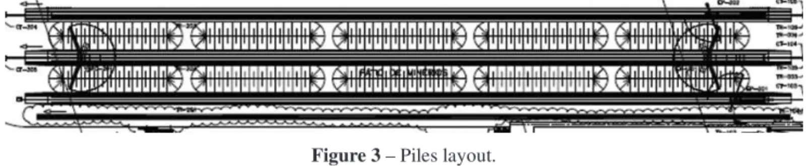
It is considered that the yard can contain 20 piles of ore with capacity for 90 Ktons each. The total static capacity of yard storage is, therefore, 1,800 Ktons. Each pile will only be able to contain one type of ore. Figure 3 illustrates the nomenclature of each pile. Odd-numbered piles are located in the top line while even-numbered piles, on the bottom line.
Figure 3– Piles layout.
The recovery rate for reclaimer is modeled with a triangular distribution of minimum values, most likely, and maximum (e.g. (6.4; 8; 9.6) Kton/h). For the Capesize, for each 10 Kton of cargo in a hold (weight of the passage of the hold), the ship loader of shipment must move to another hold to load in order to maintain the hydrostatic balance of the ship. Two bucket wheels cannot be positioned on the same pile, neither in front of the other nor next to.
The TBF (time between failures) is modeled by a negative exponential distribution with average equal to the MTBF (mean time between failure), while the TTR (time to repair), with a constant distribution, with minimum and maximum values. The same break structures for each equipment of the same type are considered.
Two types of operational unavailability are considered: unavailability for navigation caused by waves and winds and unavailability for full operation of yard (stacking and recovery) caused by winds. Both unavailabilities are modeled by a percentage, which corresponds to the number of days of operation interrupted by year. For example, if the unavailability is of 3%, then, this unavailability occurs around 11 days per year (3%×365). It is assumed that each unavailability occurs with duration of a fixed time (example 12 hours), and that the time between unavail-ability occurs according to exponential distribution. It is also considered that each unavailunavail-ability happens in specific periods of the year (for example from May to October), not occurring out of this established deadline.
The model was run in three replications in the Simul8 software, Version 20-Build 2992.
The hardware used has the following characteristics: operating system Windows 7 Professional-2009; 64-bit; Service Pack 1; Dell Manufacturer; Vostro 3450 model; IntelCoreTMi3-2310 M 2.10 GHZ CPU processor; 4 GB RAM memory; 500 GB hard disk; Intel HD Graphics Family; Number of processor cores 02; CD/DVD media drive; main monitor resolution 1366×
768; Version of DirectX 10; Network Realtek PCIe GBE Family Controller; IntelCentrino Wireless-N 1030; Bluetooth Device; Microsoft Virtual WiFi Mini.
The license is the SIMUL8 Professional 2013-Power Full-Single License-No. 1869-1338-5487-1545-4989; Elaboration of Templates; XML Simulations; Creating animated objects and sharing via website; Free Preview of models through the Simul8 Viewer; Variables manipulation of operation with significant production capacity tests.
A simulation run with 50 replications was tested, and it was clearly realized that the results showed insignificant differences when compared with three replications; that is why all the sim-ulation runs were made with only three replications.
3.3 Configuration of the simulated experiments and evaluation method
In order to determine the best distribution function of arrival of ships to be used in the simulation of a “green field” project, a database of a port terminal in Brazilian southeastern, specialized in iron ore, was used. This database contains the date and time of arrival of ships operated between December 1997 and January 2008. From this database, eight different periods of consecutive arrivals were taken. Seven periods taken had as starting dates the ones from Table 2, with 230 ships. The eighth, also from this Table, was taken from the whole database, with 2,518 records in sequence.
These eight sets were taken to the StatFit statistical module of the Simul8 software, and their results were compiled in Table 3, which shows the function that best adheres to each dataset. StatFit provides the value of p-value for each dataset analyzed. At this work, the significance level chosen wasα=0.05 and the following hypothesis was adopted:
Table 2– Periods of consecutive arrivals of ships.
Period Period of arrivals Number of ships 1 From December 21, 2003 to November 04, 2004 230 2 From May 25, 2004 to March 04, 2005 230 3 From February 15, 2005 to November 15, 2005 230 4 From February 18, 2006 to October 13, 2006 230 5 From October 05, 2006 to May 20, 2007 230 6 From December 31, 2006 to September 14, 2007 230 7 From May 12, 2007 to January 02, 2008 230 8 From December 31, 1997 to February 01, 2008 2,518
Table 3– Functions which best adjusted to each period of data.
Period Function more adjusted p-value Rank Anderson-Darling (0 to 100%) 1 Pearson 6 (0.429, 1.14, 14.2) 0.689 94.3 2 Pearson 6 (0.111, 1.37, 6.08) 0.990 100 3 All functions were rejected – – 4 Weibull (0, 0.93, 24.1) 0.996 100 5 Exponential (0, 23.8) 0.784 83.8 6 Beta (0.159, 1.04, 5.49) 0.809 100 7 Beta (0.135, 1.09, 4.98) 0.952 100 8 Pearson 6 (0.301, 1.09, 10.5) 0.438 85.5
According to Chwif & Medina (2010), the usual criteria for classifying the p-value admit to 0.10 < p-value, there is weak or no evidence against the hypothesis of adherence to the data set.
Therefore, there are no reasons to reject that adherence hypothesis to the eight dataset of Table 3, except to the Period 3, when all functions were rejected.
Additionally, for each dataset, StatFit order all adherent functions in rank and the one that gets the maximum percentage can be chosen.
The Pearson 6, among these functions, is the one that adheres better to the sets of data three times, that is, 38% of the total. Moreover, the Beta function, which appears twice (25%), is a function with ability to adapt to various forms, being used as approximation. By its parameters, it can be noticed that, in both cases, it assumes a profile close to Pearson 6 functions.
were considered adherent according to the accepted hypothesis. However, Pearson 6 of Period 8 was chosen because it fits all 2,518 records of whole dataset.
Table 4– Functions adopted for the arrival of ships.
Order Function adopted p-value Rank Anderson-Darling 1 Pearson 6 (0.301, 1.09, 10.5) 0.513 85.5 2 Weibull (0, 0.93, 24.1) 0.996 100 3 Exponential (0, 23.8) 0.784 83.8 4 Erlang (0, 1, 34.4) 0.513 50.3
This work used a very simple method to achieve its aim. It was taken a simplified and represen-tative model of a port terminal for shipment of iron ore and fixed all its operating parameters to achieve the simulated experiments. For all simulation run, the amount of ore that comes annually in the system is approximately the same, so that the amount that comes out is also nearly equal. Then, the performance of this terminal has been simulated in four ways, alternating in each one, the distribution function of arrival of ships. The functions used were those of Table 4.
The results were evaluated through the output variables of the simulation model: Demurrage, Berth Occupation, Average Queue of Ships and Lead Time. Special emphasis was given to the impact of the arrival function on the demurrage, since it is one of the most focused elements by the administrators of the port terminals, serving as a basis for making decisions about capac-ity sizing of equipment in new projects, or on investments in improvements or acquisitions in projects in operation.
4 RESULTS AND DISCUSSION
As proposed in the Introduction, different runs of the system were implemented, testing the re-sults arising from various distribution functions of arrival of ships in the simulation. The function of ships arrival, kept all the other conditions of the system, was modified in order: Pearson 6, Exponential, Erlang and Weibull.
From the simulation runs, spreadsheets with multiple items of control, important to the terminal performance, such as queues, equipment utilization rates, average inventory products, inventory turn, downtime, etc., were generated. These spreadsheets are attached after the references.
Table 5 summarized the values assumed by these dependent variables as a function of the in-put variables, that is, the functions ships arrival distribution assumed for this test: Pearson 6, Exponential, Erlang and Weibull.
Table 5– Summary of the main output variables in function of the input functions.
Variable Arrival distribution function
Pearson 6 Exponential Erlang Weibull Demurrage (US$×1.000) 62,232.86 68,216.06 90,931.06 413,585.81 Occupation of the berth (%) 47% 48% 50% 50% Average queue (No. of ships) 9.24 9.41 13.29 58.20 Average Lead Time (hours) 415.60 447.36 585.04 2,459.76
The Pearson 6 function will be referred from now on as basic function, for which all others will be compared in order to facilitate the analysis of the results. It was chosen for being the most adherent function to the database containing 2,518 consecutive ships arrivals. From Table 5, the graphs from Figures 4 to 7, which show the following comparative results, were generated.
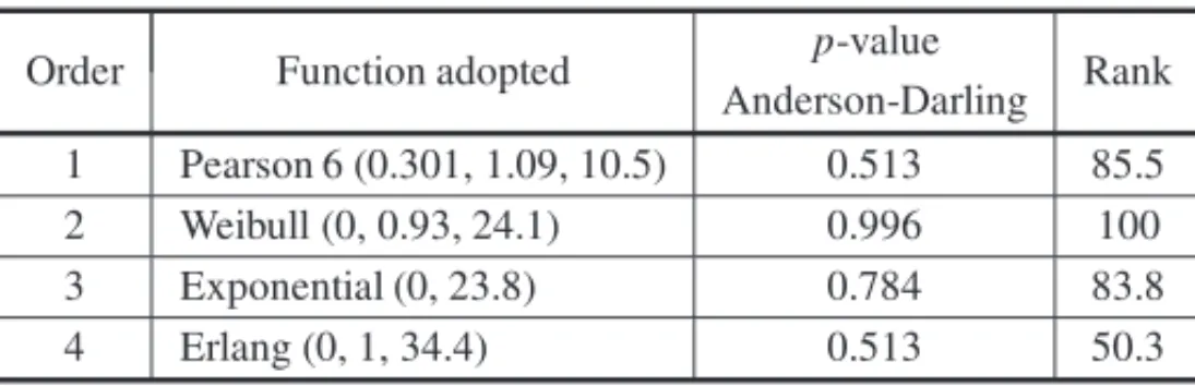
Figure 4– Graph of the absolute demurrage and percentage variation in relation to the base function (Pearson 6).
First, the average demurrage presented significant variations when compared to the base function, Pearson 6, with the others, as shown by the graph of Figure 4. Further, these differences will be analyzed in detail.
Figure 4 also showed the comparison of the percentage changes (% V) of a variable relative to the others for each of the input functions. The% V was calculated by Equation 1, where the reference variable was called old variable (OV) and the others, new variables (NV).
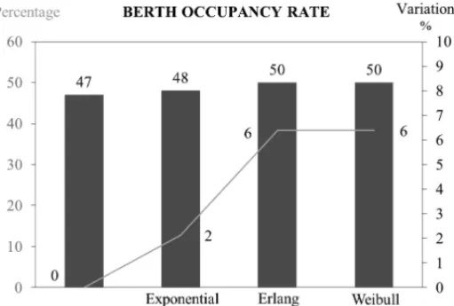
Figure 5– Graph of absolute average queue of ships and percentage variation in relation to the base function (Pearson 6).
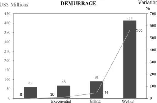
Figure 6– Graph of the occupancy rate of berth and its percentage of variation in relation to the base function.
In the graph of Figure 5, it can be observed that the average queue of the ships followed the same model of the demurrage, with percentage variation in relation to the base in the same level that the variations of the demurrage. That is quite consistent, since, as described, the demurrage was greatly affected by the waiting time for mooring.
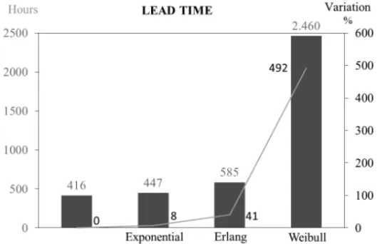
Figure 7– Average lead time graph and of the variation in relation to the base function.
also affected by the performance of the storage yard, because the product type for a given ship might not be completely available, causing impact on the service to the queue. Variations related to the base function were, respectively, of 8%, 41% and 492%, for the Exponential, Erlang and Weibull.
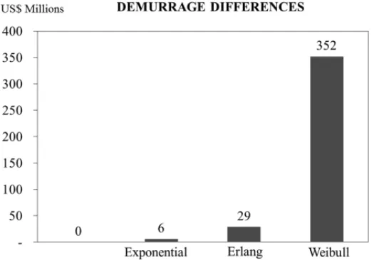
Returning to the analysis of demurrage, Table 6 showed its differences to the four functions of arrival of ships. Based on it, Figure 8 displayed the absolute difference in relation to the base function. The difference of demurrage between the Exponential function and the base (Pear-son 6) was, in absolute terms, of US$6.0 million (10% higher). Similarly, the Weibull function presented differences of US$28.7 million (46%), and the Erlang, US$352 million (565%).
Table 6– Differences of demurrage related to the base function.
Variable Distribution of arrival function
Pearson 6 Exponential Erlang Weibull Demurrage (US$×1.000) 62,232.86 68,216.39 90,931.06 413,585.81 Difference of demurrage to Pearson 6 0 5,983.53 28,698.19 352,113.81 Difference of demurrage to Pearson 6 (%) 0% 10% 46% 565%
There is a statistical issue to be considered: the confidence intervals of the results of the analyzed variables might have overlapping ranges. This led to the conclusion that, statistically, it cannot be said that a result is worse than other one. However, in practice, the managers who have to make decisions are obliged to consider the averages as the most probable values and decide by them.
Figure 8– Graph of the demurrage absolute difference among other functions and the base.
average demurrage using other functions, in relation to the Pearson 6, it could be purchased two or more machines of yard. These ones are essential to the operations and such acquisition could significantly increase production and terminal performance, reducing demurrage.
Therefore, the result of a simulation can induce a manager of projects to increase the capacity of the system equipment or introduce additional equipment in order to reduce the average value of annual demurrage at the terminal. After all, US$28 million or more of demurrage, if they can be saved with an investment that pay itself in one year, will certainly be transformed into increase of capacity. Even the US$6.0 million difference, in the case of the Exponential function, would pay a machine in three years.
Finally, all the questions presented in Item 2.3 can be, now, answered. Regarding the first of them, about the importance of the input functions in the simulation, we found that they clearly influence the results in a very significant way. Some software used for the elaboration of simulation models do not have the Pearson function. The need to use statistical software to determine these functions with greater precision becomes clear.
Concerning the level of impact that the choice of representative functions of arrivals has on the results, results can be obtained with variations of up to 566% in predicting demurrages paid to ships and of 530% in average queue, being these two the main parameters used in the evaluation of results of this type of simulation.
There is no doubt that the results may induce the executives of companies to take bad decisions because of the very large variation referred to above.
5 CONCLUSIONS
In modern simulations, in addition to the operational performance results, the focus has also turned to the financial results, when these are able to be evaluated in the model. Project managers have to take quick and high impact decisions based on their results. Therefore, the simulations must have a sufficiently high degree of accuracy to the decision-making process.
As already seen, studies on ports and port terminals have admitted that the statistical distribution of arrival of ships is strongly influenced by controls as rules of priority. Shipowners also delay or advance their ships travelling in order to reduce the waiting time for mooring. This makes distribution functions such as Exponential, Erlang and Weibull, although generally recommended to represent the arrival of ships in a port, to be used carefully.
As demonstrated, the statistical distribution functions used as input data in simulations of pro-cesses impact heavily on their results, and may lead to wrong decisions to business executives who may use them. In relation to simulations of ship operations in port terminals of iron ore shipment, it was proved that results with variations of up to 566% in prediction of demurrages paid to ships and 531% on average queue can be obtained. In relation to simulations of ship operations in port terminals for shipment of iron ore, it was shown that results with variations of up to 565% in predicting demurrage paid to ships, and of 531% in the middle queue can be obtained.
It was also demonstrated that, despite the recommendation of traditional literature, the Exponen-tial, Erlang and Weibull functions may not be the most appropriate to represent the arrival of ships in a shipping terminal of iron ore. Note that the majority of published works does not bring in detail the parameters of statistical functions used in simulation models. It would be very use-ful if this became a constant practice. Models such as the IDEF-SIM can help a lot in recording these parameters, allowing their replication, especially for using in green field projects.
Finally, it is recommended more databases of Brazilian port terminals of iron ore to be searched. As, in Brazil, there is difficulty in obtaining data from companies, it has been suggested, as an alternative, these data to be requested to associations like the ABTP – Brazilian Association of Port Terminals. These associations may compile enterprise data; they are reliable sources and can preserve confidentiality of their members. In addition, government agencies such as the ANTAQ – National Agency of Waterway Transportation – can take charge of maintaining such databases.
ACKNOWLEDGMENTS
REFERENCES
[1] ALIZADEHAH & TALLEYWK. 2011. Microeconomic determinants of dry bulk shipping freight rates and contract times.Transportation,38(3): 561–579.
[2] BANKSJ, CARSONJS, NELSONBL & NICOLDM. 2010. Discrete-event System Simulation, 5thed. Prentice-Hall: Englewood Cliffs, NJ.
[3] BUGARIC´ U & PETROVIC´ D. 2007. Increasing the capacity of terminal for bulk cargo unloading. Simulation Modeling Practice and Theory,15(10): 1366–1381.
[4] BUGARIC´U, PETROVIC´D, JELIZV & PETROVICDV. 2012. Optimal utilization of the terminal for bulk cargo unloading.Simulation,88(12): 1508–1521.
[5] CAMELOGR, COELHOAS, BORGESRM & SOUZARM. 2010. Teoria das filas e da simulac¸˜ao aplicada ao embarque de min´erio de ferro e manganˆes no terminal mar´ıtimo de Ponta da Madeira. Cadernos do IME: S´erie Estat´ıstica,29: 1–16.
[6] CANONACOP, LEGATOP, MAZZARM & MUSMANNOR. 2008. A queuing network model for the management of berth crane operations.Computers & Operations Research,35(8): 2432–2446. [7] CASACAACP. 2005. Simulation and the lean port environment.Maritime Economics & Logistics,
7(3): 262–280.
[8] CHWIFL & MEDINA AC. 2010. Modelagem e Simulac¸˜ao de Eventos Discretos – Teoria e Apli-cac¸˜oes, Terceira Edic¸˜ao, Ed. Bravarte.
[9] CASSETTARIL, MOSCAR, REVETRIAR & ROLANDOF. 2011. Sizing of a 3,000,000 t bulk cargo port through discrete and stochastic simulation integrated with response surface methodology tech-niques.Proceedings of the 11th WSEAS international conference on Signal processing, computational geometry and artificial vision, p. 211–216.
[10] CIGOLINIR, MARGHERITAP & TOMMASOR. 2013. Sizing off-shore transhipment systems: a case study in maritime dry-bulk transportation.Production planning & control,24(1): 15–27.
[11] DEMIRCI E. 2003. Simulation modelling and analysis of a port investment. Simulation, 79(2): 94–105.
[12] DRAGOVIC´B, PARKNK, RADMILOVIC´Z & MARASˇV. 2005. Simulation modelling of ship-berth link with priority service.Maritime Economics & Logistics,7(4): 316–335.
[13] DUINKERKENMB, DEKKERR, KURSTJENSJA, OTTJESNP & DELLAERTNP. 2007. Comparing transportation systems for inter-terminal transport at the Maasvlakte container terminals. New York: Springer Heidelberg.
[14] FLEURYPF & HIJJARMF. 2008. Logistics overview in Brazil 2008.Instituto ILOS. Available in:
<http://www.ilos.com.br/index2.php?option=com docman&task=doc view&gid=31&Itemid=44>
[15] HOMW & HOKHD. 2006. Risk management in large physical infrastructure investments: the con-text of seaport infrastructure development and investment.International Journal of Maritime Eco-nomics (IJME),8(2): 140–168.
[17] KIMKH, LEEKM & HWANGH. 2003. Sequencing delivery and receiving operations for yard cranes in port container terminals.International Journal of Production Economics,84(3): 283–292. [18] LAWAM. 2007. Simulation modeling and analysis. 4th ed. New York: McGraw-Hill.
[19] LEAL F, COSTA RFS, MONTEVECHIJAB, ALMEIDA DA & MARINSFAS. 2011. A practical guide for operational validation of discrete simulation models.Pesquisa Operacional(Impresso),31: 57–77.
[20] LEGATOP & MAZZARM. 2001. Berth planning and resources optimization at a container terminal via discrete event simulation.European Journal of Operational Research,133(3): 537–547. [21] LIUY & TAKAKUWAS. 2011. Modeling the materials handling in a container terminal using
elec-tronic real-time tracking data. In:Winter Simulation Conference.
[22] MEISELF & BIERWIRTHC. 2009. Heuristics for the integration of crane productivity in the berth allocation problem. Transportation Research Part E: Logistics and Transportation Review, 45(1): 196–209.
[23] MONTEVECHIJAB, LEALA, PINHOA, COSTARF, OLIVEIRAML & SILVAAL. 2010. Concep-tual Modeling in Simulation Projects by mean adapted IDEF: an Application in a Brazilian company. In:Proceedings of the Winter Simulation Conference.
[24] MONTGOMERY DC. 2009. Design and Analysis of Experiments, 6th ed, John Wiley and Sons, Arizona, USA.
[25] NISHIMURAE, IMAIA & PAPADIMITRIOUS. 2001. Berth allocation planning in the public berth system by genetic algorithms.European Journal of Operational Research,131(2): 282–292. [26] OTTJESJA, VEEKEHP, DUINKERKENMB, RIJSENBRIJJC & LODEWIJKSG. 2007. Simulation
of a multiterminal system for container handling. In: Container terminals and cargo systems. New York: Springer Heidelberg, p. 15–36.
[27] PACHAKISD & KIREMIDJIANAS. 2003. Ship traffic modeling methodology for ports.Journal of Waterway, Port, Coastal, and Ocean Engineering,129(5): 193–202.
[28] PSARAFTISHN & KONTOVASCA. 2014. Ship speed optimization: Concepts, models and combined speed-routing scenarios.Transportation Research Part C: Emerging Technologies,44: 52–69. [29] PAROLAF & SCIOMACHENA. 2005. Intermodal container flows in a port system network: Analysis
of possible growths via simulation models.International Journal of Production Economics,97(1): 75–88.
[30] SARGENTRG. 2013. Verifications and Validation of Simulations Models.Journal of Simulation,
7(1): 12–24.
[31] SCHOFIELDJ. 2011. Laytime and Demurrage. 6thed. Taylor and Francis Group.
[32] SHABAYEKAA & YEUNGWW. 2002. A simulation model for the Kwai Chung container terminals in Hong Kong.European Journal of Operational Research,140(1): 1–11.
[33] TAHARRM & HUSSAINK. 2000. Simulation and analysis for the Kelang container terminal opera-tions.Logistics Information Management,13(1): 14–20.
[35] UNITED NATIONSCONFERENCE ON TRADE AND DEVELOPMENT(UNCTAD). 1985. Port de-velopment: a handbook for planners in developing countries. New York: United Nations, p. 108– 128. Available in: <http://r0.unctad.org/ttl/docs-un/td-b-c4-175-rev-1/TD.B.C.4.175.REV.1.PDF>.
Accessed on: 20/03/2014.
[36] VANASPERENE, DEKKERR, POLMANMTH & SWAANAH. 2003. Allocation of ships in a port simulation. In: VERBRAECKA & HLUPICV. (Eds.), Simulation in industry – Proceedings of the 15th European Simulation Symposium, Delft, p. 26–29.
[37] VANVIANENT, MOOIJMAND, OTTJESJ, NEGENBORNR & LODEWIJKSG. 2012. Simulation-based operational control of a dry bulk terminal. Networking, Sensing and Control (ICNSC), 9th IEEE International Conference, p. 73–78.
[38] WANKEP. 2011. Ship-Berth Link and Demurrage Costs: Evaluating Different Allocation Policies and Queue Priorities via Simulation.Pesquisa Operacional,31(1): 113–134.
[39] WEBBER SL. 2012. O papel do BNDES nas exportac¸˜oes brasileiras no per´ıodo 2000-2011. Reposit´orio Digital UGRGS – LUME.