A WAVELETS-BASED ANALYSIS OF THE PHILLIPS
CURVE HYPOTHESIS FOR THE BRAZILIAN
ECONOMY, 1980-2011
Edgard Almeida Pimentel*
Published in Honour of Professor Raul Cristóvão dos Santos
Abstract
This paper implements a wavelets-based analysis of the Phillips curve hypothesis — as formulated by Friedman and Phelps — for the Brazilian economy, concerning the last thirty years. We provide an introductory dis-cussion on Phillips curve’s main arguments and an exploratory data anal-ysis for the variables under consideration: prices, unemployment and real wages. In the sequel, we estimate variances and correlation structures be-tween these aggregates through wavelets. Our findings reject the Phillips curve hypothesis for the Brazilian economy in the short run while sug-gest that it does hold in the long run. Finally, the correlation structure obtained in the paper captures particular aspects of Brazilian economic policy within the period.
Keywords:Phillips curve; Brazilian economy; Wavelets.
Resumo
Este artigo desenvolve uma análise da hipótese da curva de Phillips — de acordo com a formulação de Phelps-Friedman — para a economia brasileira dos últimos 30 anos através da metodologia de ondaletas. Uma introdução às ideias fundamentais do argumento de Phillips é seguida por uma breve exposição dos principais desenvolvimentos teóricos no tema e uma discussão acerca do recente panorama da pesquisa no Brasil. Em se-guida, uma análise exploratória das variáveis em questão é empreendida. Por fim, são apresentadas estruturas de correlação e variâncias estimadas através da metodologia de ondatelas, desagregando assim efeitos de curto e longo prazo. Nossos resultados rejeitam a hipótese da curva de Phillips para a economia brasileira no curto prazo enquanto sugere a sua validade no longo prazo. Ainda discutem-se aspectos da pol+itica econômica naci-onal evidenciados pela metodologia de análise empregada.
Palavras-chave:Curva de Phillips; Economia Brasileira; Ondaletas. JEL classification:C10, E30, E42
*Center for Mathematical Analysis, Geometry, and Dynamical Systems, Departamento de
Matemática, Instituto Superior Técnico, Lisboa, Portugal. E-mail: [email protected]
1
Introduction
Phillips curve reasoning is familiar to most undergraduate students in Eco-nomics: an allegedly negative correlation between unemployment and infla-tion which could not be empirically rejected until the 60’s. After that (as pointed by Gordon 2008) transformations in the macroeconomic scenario put Phillips curve under probation and, like other arguments, it sounded as one of the fairy tales from the very early beginning of Macroeconomics thought.1
Meanwhile, during the 70’s, Friedman and Phelps argued that Phillips for-mulation would not be completely disposable. In fact, the negative trade-off between inflation and unemployment should be expected to hold in the short-run — since, in the long run, monetary neutrality and adjustments in the labour market would prevent such relationship to be empirically verified. Unlike Phillips’ original argument, Friedman and Phelps derived their con-clusion deductively, and gave rise to a new sort of problem: how could one properly test Friedman-Phelps (FP) hypothesis? It would require an empir-ical method to separate long-term from short-term effects comprised by the same signal, or time series. Many attempts to pursue this methodology have been undertaken, e.g. vectorial auto-regressive models and forecast analysis and even causality tests, leading to unfortunate misunderstandings - simply because the answer did not fit the question.2
Fortunately, in which concerns isolating short-run from long-run compo-nents of a time series the Economics profession has at hand the wavelets ma-chinery. Decomposing a signal — 1D in the case of a time series — in wavelets coefficients may shed a light on distinct (low and high) frequencies, corre-sponding to long and short term effects.
In this paper, we test the hypothesis due to Friedman and Phelps — failure of Phillips curve in long-run and its validity in short-run — for the Brazilian economy in the period between 1980 and 2011, either for the entire period as well as for three distinct sub-periods. These sub-periods are chosen according to major events in Brazilian economic environment. The first one (January 1980 to June 1994) intends to specialize the analysis for the so-called lost-decade — as well as capture particular impacts of hyperinflation and debt crisis. The second period (July 1994 to December 2002) opens with the Plano Real and covers the following efforts in monitoring inflation. The final sub-period (January 2003 to February 2011) covers Lula da Silva’s government and, ultimately, captures the correlation structure for the most recent years.
Section two of the paper discusses some historical aspects of the Phillips curve and the FP hypothesis as well as presents a brief review of the Brazilian case. A third section approaches the wavelets methodology while a fourth one presents some exploratory data analysis. Finally, section five presents correlation results followed by some concluding remarks.
2
Once upon a time...
In this section we present a brief discussion on the Phillips curve. The first subsection discusses the very early beginning of this idea and some of its
em-1For instance the so-called Haavelmo theorem which is everything but a Theorem.
2Particularly unfortunate examples in this literature are due to Kitov (2009), Kitov (2006)
pirical spillovers in the international literature. A second subsection briefly discusses the Brazilian case.
2.1 The very early beginning
Economica, 1958: the New-Zealand born British economist Alban W. Phillips publishes an article entitledThe relation between unemployment and the rate of change of money wage rates in the United Kingdom. Concerning the dataset, the paper covers three sub-periods ranging from 1861 to 1957 (1861-1913, 1913-1948 and 1913-1948-1957). It is worthy of note how the author remarkably refined theoretical premises. Firstly, Phillips argues that, if any, the relation between unemployment and variations in wage rates should be of a non-linear nature. This would be implied by rigidity of wage levels — by worker reluctance or legal restrictions.
Formally, this assumption entails the following ODE:
˙
w(t) =f (u(t)) (1)
wheref is a non-linear function of the unemployment levelu(t) andw(t) is the wage level. Secondly, Phillips assumes the influence also of variations in unemployment rate — although he does not specify the nature of this rela-tionship. We may assume it to be given by
˙
w(t) =f (u(t),u˙(t)) (2)
or
˙
w(t) = f (u(t)) ˙
u(t) = g(w(t))
Under (2) inflation may be understood as a Lagrangian of position and velocity generating a functional to be minimized over some function space.
It shall be clear that such formulations incorporate demand components of wage rates variation. However it neglects the supply-side components. That is precisely Phillips’ third assumption: wages should represent most, but no all production cost. The consequence would be that in a capital-labour produc-tion model, in order to increase wages, an increase rate in capital cost should be higher than productivity growth by an amount that is precisely the labour intensity in production. Roughly speaking, suppose a Cobb-Douglas produc-tion funcproduc-tion given byΠ(L, K) =LαKβ.
Following Phillips then, an increase in capital cost in order to influence wage levels should be such that ˙cL·α6c˙K(t).
Phillips, assuming so, was foreseeing the supply relevance in (PC) claimed to be integrated 20 years later.
From an empirical point of view, Phillips’ article cannot reject the negative correlation between unemployment and inflation for the century-long period under analysis.
Samuelson & Solow (1960) named Phillips’ evidences after him asPhillips curveand entailed an anti-inflation analysis of his conclusions3. In this paper, 3Samuelson and Solow lamented the lack of analogous empirical studies for the American
two major developments take place. The first one is the menu that Economic policy may take advantage of: some amount of inflation in benefit of lower unemployment and, perhaps, even vice-versa. Furthermore, the authors also launched the basis for Friedman-Phelps hypothesis, arguing that high unem-ployment levels would either require huge increments in inflation to be re-versed or lead to a positive relationship between both variables, reversing then the nature of the correlation found by Phillips.
After the empirical failure of the Phillips curve, around mid 60’s, Fried-man and Phelps4suggested that adjustments in agents’ expectations, as well as distortions entailed by policy-makers attempts to reduce unemployment rate below the so called natural rate, would jeopardize in the long run the neg-ative relationship between unemployment and inflation. Lucas (1972) and the idea of rational expectations also reinforced the relevance of FP arguments.
Since late 70’s, many efforts have been taken in order to test and shed a light on the correlation structure between prices and unemployment or wages and unemployment. Most of these studies are focused, however on method-ologies unable to isolate short from long-run components and, hence natu-rally shall fail in provide robust empirical results.
From the theoretical perspective, many attempts to read beyond Phillips’ ideas address somehow the issue of the correlation between these variables. A new-Keynesian approach was suggested independently by Taylor (1980) and Calvo (1983) and further developed by Mankiw (2001) and Dew-Becker & Gordon (2005). For a detailed and involving survey on historical aspects of Phillips curve, we refer to Gordon (2008).
2.2 Phillips curve and the Brazilian economy
Concerning the investigation of the Phillips curve for the Brazilian economy, many efforts have been undertaken to enhance the understanding of the pro-fession on the topic. Meanwhile, to the best of our knowledge, there are no works that approach this issue through the framework of wavelets.
In its vast majority, these studies contribute to the literature by consider-ing the effects of additional explanatory variables or by deriving specifications from alternative theoretical frameworks. An example of the former class is Schwartzman (2006). In an ambitious — successful though — paper, the au-thor compiles the most significant formulations for the Phillips curve in the context of the Brazilian economy as well as implements a variety of empirical models. These are estimated through 3SLS — three stages least squares. Ei-ther Schwartzman (2006) as the references Ei-therein, provide the relevant argu-ments around which the debate concerning the Brazilian Phillips curve have evolved. Meanwhile, since the method of 3SLS is not able to disaggregate the various temporal components of the analysed time series, the study falls short in the evaluation of the dichotomy between short and long run that is inherent to the Phillips curve.
Examples of the latter class of studies are represented by the papers of Caetano & Moura (2012) and Mazali & Divino (2010). Both studies investi-gate the so-called New Keynesian Phillips Curve (NKPC). In Mazali & Divino (2010) the authors estimate an under-identified model through the General-ized Method of Moments. The authors claim to isolate the short-run trade-off
and investigate both real wage rigidity and the validity of restrictions imposed by the theoretical framework. However, the scope of the employed method-ology does not allow the authors to isolate the short-run trade-off. Indeed, it captures only marginal variations in time domain — not in frequency do-main. Moreover, the use of dummy variables to account for the presence of unit roots remove the time-location property of the estimators.
On the other hand, Caetano & Moura (2012) also proposes an estimation of the NKPC. The authors explicitly states the hypothesis that information diffuses slowly among the economic agents. In their formulation, a proxy variable for expected inflation in the future is required. To circumvent this problem, the median of the market projections of inflation is used — it im-proves the previous techniques which used out-of-sample forecasting from VAR models5. Although improving our understanding about the role played by rigidity information in the Philips curve, the paper also collapses all the different frequencies — running from short to long run — into a point.
The advantages of using the wavelets-based machinery are clear in this setting. Firstly, there is no need for further investigation concerning non-stationariness or asymmetric, non-normal distributions. Secondly, and more important, this framework allows us to decompose the information under analysis in frequency domain unravelling the distinct contribution of larger and smaller time horizons to the series.
3
Wavelets methodology and dataset
3.1 The wavelets machinery
Connecting wavelets-based methods with time-series has recently provided a powerful analytical framework. Important theoretical accomplishments as well as a systematic exposition on this subject are due to Percival (1995), Per-cival & Guttorp (1994), PerPer-cival & Mofjeld (1997), PerPer-cival & Walden (1993), Percival & Walden (2006) and Morettin (1999).
The use of wavelets-based techniques in Economics has been explored within the financial context. Among the numerous references one may sug-gest Rua & Nunes (2009), Dew-Becker & Gordon (2005), Gallegati (2008) and Gallegati & Gallegati (2007). The Brazilian case is approached by Pimentel & da Silva (2011). In many other branches of Science, such functions are also of huge relevance: image processing, stochastic calculus, measure theory and even harmonic analysis.6
Wavelets machinery provides a powerful analytical tool in dealing with time series for many reasons. Firstly, the eigenvalues of the lag operator are not required to be inside the unit circle in C; i.e., wavelets do not require unit root considerations. Moreover, in studying correlation and variance struc-tures, one may be interested in different components aggregated in the signal: short and long-run aspects which can be isolated through distinct frequen-cies of wavelets transform. In this concrete case, testing FP hypothesis means nothing but decompose unemployment and inflation in short and long term components.
Roughly speaking, a wavelet is a function satisfying specific properties. One of this property relates the function integral with its dilations — enabling us to construct wavelets families. On the other hand, these same properties characterizes certain wavelet families as orthonormal basis of the space of square integrable functions,L2(R). The natural procedure is then to embed a time series in an appropriateL2 and address it as its coefficients in wavelets. We give rigour to the previous comments in which follows.
Definition 1. A functionφ:R−→Rsuch that Z
R
φ(s)ds= 0
and
Z
R
φ(s)2ds= 1
is called a wavelet. If, furthermore, its Fourier transform
F(φ) (ξ) =
Z
R
φ(s)e−2πi(s·ξ)ds
is such that
Cφ= Z
R+
F(φ) (ζ)
ζ dζ∈(0,+∞) (3)
φis said to be admissible.
Notice that the set of wavelets is closed under dilations and translations. The first one is due to the change of variables formula while the second one is due to translation invariance of the Lebesgue measure. The starting point in dealing with wavelets is the Continuous Wavelet Transform (CWT). This procedure investigates the change of a particular function in a particular point of time at a certain scale. For instance, consider we have a signal x(t) and we want to understand the its behavior at timet∗ in scalej according to a particular wavelet functionφ. Firstly, we compose a dilation (corresponding to the scale) and a translation (corresponding to time) in the following way
Dilj◦τt∗(φ) (s) = (j)− 1 2φ s−t
∗
j !
and then obtain the (CWT) at those points
W(j, t∗) =
Z
R
x(s) (j)−12φ s−t ∗
j !
ds (4)
n
2j:j= 1, ...,log2Jo
where⌊·⌋ denotes the floor function, returning the largest integer below its argument, i.e.,
⌊x⌋=y∈N:y+ 1≥x
Moreover, the translations are also limited to point in time of the form
t∗=k 1
2j (5)
DWT relies basically on two finite families of wavelet functions — also called filters — with lengthL,a fixed positive integer. They are called mother and father wavelets, represented respectively by the collections
{hl:l= 0, ..., L−1}
and
{gl:l= 0, ..., L−1}
Additionally, they are supposed to satisfy
L−1 X
l=0 hl= 0
and
L−1 X
l=0 gl = 1
The class of mother wavelets also satisfies an additional condition related to shift-independence, given by
L−1 X
l=0
hlhl+2n= 0∀n∈N
Mother and father wavelets serve distinct purposes: the former one aims to capture deviation effects while the latter one’s goal is to capture low-frequency components of the signal.
Given these families of functions and a time series {x(t) :t= 1, ..., T}one can proceed the wavelet decomposition, which evokes the pyramid algorithm. Put simply, one starts by computing a first collection of high and low fre-quency coefficients, i.e.,
ω1(t) = L−1 X
l=0
(hlx) (s) (6)
and
υ1(t) = L−1 X
l=0
wheres˙= 2t+ 1−l; modT.
ω1contains high-frequency information aboutxwhereasυ1provides the
scaling coefficients regarding the first level of decomposition. Definition ofs suggests that both vectors obtained by (6) and (7) have half the length of the original time series. In particular, we could replicate (6) and (7) regardingυ1.
It would provide us with
ω2(t) = L−1 X
l=0
(hlυ1) (s)
and
υ2(t) = L−1 X
l=0
(glυ1) (s)
At this stage, ω2andυ2have the same interpretation as before, but now
with only a quarter of the original length. Proceeding inductively, one gets the matrix
Γ(x)h ω1 · · · ωJ υJ i
which returns the DWT of the signalx.
A natural question concerns the dyadic limitation entailed by DWT. There are several drawbacks: dyadic length, dyadic scaling and dyadic-dependent temporal translation. Clearly, if a dataset has length 2k+ 2 (andk is not 1, of course) it is not reasonable to discard 2 observations and lose information. Furthermore, if we are particularly interested in a time instant which does not satisfies (5) we may also lose important insights and decrease our analytical abilities.
To circumvent these dyadic impediments, we discuss the Maximal Over-lap Discrete Wavelet Transform (MODWT). Instead of consider only dyadic-dependent translations, MODWT allows for any integer translation within the time interval under consideration. The transition from DWT to MODWT is fairly simple; the MODWT matrix is given by
eΓ(x) =h ωe1 · · · ωeJ υeJ i (8)
where
e ω1(t) =
L−1 X
l=0
(hlx) (s)
and
e υ1(t) =
L−1 X
l=0
(glx) (s)
are computed fort= 1, ...T ands=t−l modT. As before, the pyramid algo-rithm is implemented to provide us with the rest of the decomposition, until theJ-th level. We observe that, in this case,Jmay be any integer from 1 to the signal length.
Definition 2. Letx(t)be a signal andωejitsj-th scale wavelet coefficients obtained
by MODWT decomposition. Then, if finite, the time-dependentj-th wavelets vari-ance ofx(t)is given by
ν(x, j, t) = varωej(t)
Ifνdoes not depend ont, it is called the time-independentj-th wavelets vari-ance ofx(t)and is denotedν(x, j)ν(x, j, t).
Definition (2) can be generalized in the natural way to the context of co-variances. In fact we have the
Definition 3. Letx(t)andy(t)be two, possibly identical, signals of same length. Then, thej-th wavelets covariance of(x(t), y(t))is given by
νx,y(j, t) = cov
e
ωx,j(t),ωey,j(t)
As usual, covariances may be normalized to thej-th wavelets correlation coef-ficient betweenx(t)andy(t), given by
ρx,y(j, t) =
covωex,j(t),ωey,j(t)
varωex,j(t)
varωey,j(t)
= νx,y(j, t)
ν(x, j, t)ν(y, j, t)
Both definitions (2) and (3) are based on Percival & Walden (2006), as well as the correlation and variance tests implemented in this paper.
3.2 The dataset
The dataset consists of three time series. At first, the Brazilian consumer price index, IPCA, constructed by the Brazilian Institute of Geography and Statis-tics (IBGE), from January 1980 to February 2011 on a monthly basis. Secondly, the unemployment rate computed for the Metropolitan Regions from January 1980 to February 2011 also by IBGE under the employment monthly survey (PME). Finally, the rate of change of the real minimum wage, which is com-puted based on the Brazilian Real Minimum Wage through
rwrc(t) = ln [RMW(t)]−ln [RMW(t−1)]
whererwrc(t) is the real minimun wage rate of change at instanttand RMW(t) is the real minimum wage ate instantt.
Each series has 374 observations. The dataset was obtained from the server maintained by the Institute of Applied Economic Research (IPEA), the IPEA-DATA.7
4
Exploratory data analysis
We present in this section the exploratory data analysis results. Firstly, we discuss the series for the entire period (1980-2011) and in the sequel we spe-cialize the analysis for three sub-periods, namely, 1980-1994, 1994-2003 and 2003-2011.
Figure 1 shows the graph of Brazilian CPI for the entire period of analysis, which covers the hyper-inflation of the 80’s with a peak around 80%. Un-employment rates, when considered the entire period, does not exhibit the same variation pattern as CPI. In fact, during he last thirty years, the unem-ployment rate varied within 0 and 14%. Figure 2 presents the unemunem-ployment series for the entire period. On its turn, the real wage monthly variation is the most erratic variable for the period 1980-2011, concentrating the largest discrepancies in the first half of the observations.
Figure 1: Brazilian CPI, 1980-2011
Figure 3: Monthly variations of real wage, 1980-2011
We now proceed to the wavelets-based exploratory analysis, namely, the investigation of MODWT coefficients for the three variables under considera-tion.
Figure 4: MODWT, Brazilian CPI, 1980-2011
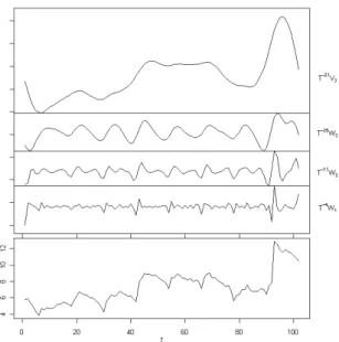
MODWT analysis for the Brazilian CPI indicates the relevance of both the short and the long-run contribution to inflation. Indeed, one could read this information as an evidence of demand and supply influence on CPI, the for-mer one acting in the short-run while the latter one would impact the long-run.
unemployment rates: both short and long-run components seems to be crucial for the signal total energy.
Figure 5: MODWT, Brazilian Unemployment rate, 1980-2011
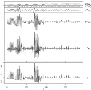
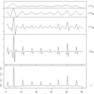
The interesting findings regard indeed the MODWT for real wage varia-tions in the entire period: only short-run coefficients seems to be effective to determine the total energy of this time-series. In other terms: MODWT provides us with strong evidences that adjustments in real wages are due to short-run components instead of long-run ones.
Figure 6: MODWT, Real wage variations, 1980-2011
sub-periods, we observe the same pattern.
Figure 7: MODWT, Brazilian CPI, 1980-1994
Figure 8: MODWT, Brazilian CPI, 1994-2003
Again one observes the influence of both short-run as well as long-run components on Brazilian price index. Now, however, one can notice that, for every period, the lower the frequency the higher the magnitude of the coeffi -cient, indicating an increasing influence of long-run components.
Figure 9: MODWT, Brazilian CPI, 2003-2011
Figure 11: MODWT, Unemployment rates, 1994-2003
As a general picture for these variables, the entire period analysis indicates both low and high frequency influences as not negligible. Meanwhile, taking into account three distinct sub-periods reveals the long-run predominance over the short-run in determining the signal.
Fortunately, it is not the scenario when dealing with real minimum wage variations.
Figure 13: MODWT, Real wage variations, 1980-1994
Figure 14: MODWT, Real wage variations, 1994-2003
Figure 15: MODWT, Real wage variations, 2003-2011
is that, when significantly distinct from zero, they do not deviate enough to at-tribute to long-run components any influence on real wage variations. These findings are consistent with those concerning the whole period and, further-more, consistent with a theory that in the short run, inflation does not see unemployment.
Next section presents variance and correlation analysis for this dataset.
5
Wavelets-based correlation structures
In this section we present the wavelets-based results concerning variances and cross-correlation regarding our dataset. The variance component of our anal-ysis reflects volatility within the data for the entire period as well as for the three sub-periods we took into consideration.
All reported values are statistically significant at 5% level. We firstly ex-amine wavelets variance for the entire period (Table 1).
Table 1: Wavelets variance, 1980-2011
Scale CPI Unemployment rate Real minimum wage variation
d1 3.684998 0.0583990 0.01079229
d2 7.752394 0.1021868 0.00532421
d3 14.79543 0.2194658 4.828657e-03
d4 20.63222 0.1633090 1.312806e-04
d5 38.02026 0.3843519 6.790213e-05
Scalesd6tod8were not statistically significant at 5%.
This is not the case for the real wage variation: indeed, in the long-run, real wage changes tend to present null volatility. It indicates that adjustments in real wage are due to short-term components instead of long-term ones, corrob-orating our findings of the previous section. We now examine the considered sub-periods.
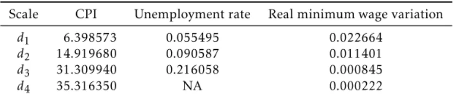
Table 2: Wavelets Variance, 1980-1994
Scale CPI Unemployment rate Real minimum wage variation
d1 6.398573 0.055495 0.022664
d2 14.919680 0.090587 0.011401
d3 31.309940 0.216058 0.000845
d4 35.316350 NA 0.000222
Scalesd5tod6were not statistically significant at 5%.
Again, CPI and unemployment present variances increasing as frequency decreases, providing evidences that long-run components of both variables present higher volatility. On the other hand, real wage variation presents sys-tematically monotone variance, indicating that volatility in real wage during this sub-period is mostly due to short-term components.
The second sub-period results are presented in Table 3.
Table 3: Wavelets Variance, 1994-2003
Scale CPI Unemployment rate Real minimum wage variation
d1 0.045928 0.088187 0.001093
d2 0.054641 0.105119 0.000324
d3 0.052034 0.216031 0.000104
Scalesd5tod6were not statistically significant at 5%.
Again, unemployment rate presents increasing volatility as we move to-wards long-run analysis. Meanwhile, CPI variance in this period remains fairly stable along the frequencies. This fact reflects the effectiveness of macro-economic policy towards monetary stability in Brazil during the years 1994-2003. Also as we should expect from previous results, real wage variations presents higher volatility concerning short-run components.
Table 4: Wavelets Variance, 2003-2011
Scale CPI Unemployment rate Real minimum wage variation
d1 0.009430510 0.039180130 0.000520659
d2 0.011051780 0.094052800 0.000281648
d3 0.013613010 0.136506200 0.000208061
Scalesd5tod6were not statistically significant at 5%.
these recent years, inflation monitoring failed to be as effective as it has been in the first eight years of Plano Real.
Furthermore, such (perhaps) careless monitoring of long-run components of Brazilian inflation may rely among the causes of the recent inflationary pressure felt by the agents in Brazilian economy since 2008. Real wage ad-justments possesses lower variances in lower frequencies, however, for this sub-period, such volatility is fairly null since the lower scale, i.e., since 2003, real wage adjustments variations are not far from zero, irrespective of short or long-run components.
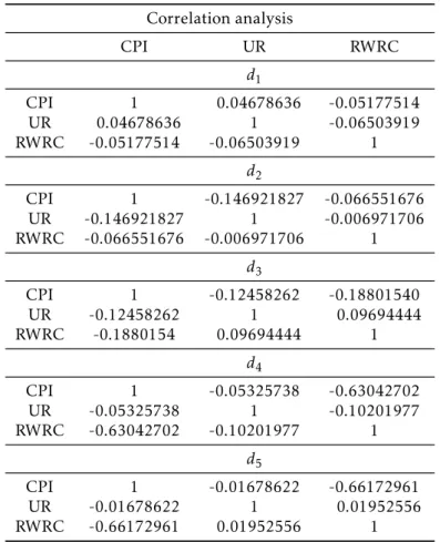
We are now in position to reach the core of our analysis: covariance and correlation results for real wage change rates, CPI and unemployment rates. Table 5 presents the results for the whole period.
Table 5: Wavelets correlation, 1980-2011
Correlation analysis
CPI UR RWRC
d1
CPI 1 0.04678636 -0.05177514
UR 0.04678636 1 -0.06503919
RWRC -0.05177514 -0.06503919 1
d2
CPI 1 -0.146921827 -0.066551676
UR -0.146921827 1 -0.006971706
RWRC -0.066551676 -0.006971706 1
d3
CPI 1 -0.12458262 -0.18801540
UR -0.12458262 1 0.09694444
RWRC -0.1880154 0.09694444 1
d4
CPI 1 -0.05325738 -0.63042702
UR -0.05325738 1 -0.10201977
RWRC -0.63042702 -0.10201977 1
d5
CPI 1 -0.01678622 -0.66172961
UR -0.01678622 1 0.01952556
RWRC -0.66172961 0.01952556 1
Scalesd6tod8were not statistically significant at 5%.
correlated with prices — which one should expect under any analytical frame-work — but such correlation gets stronger as we reduce the frequency and ad-dress long-run components. Roughly speaking, it indicates that adjustments in real wage do not see the distant future when looking at prices.
Specializing the analysis for the period between 1980 and 1994 the find-ings are quite consistent to those concerning the entire period: prices and unemployment are uncorrelated in the short-run, negatively correlated in the long-run and real wages adjustment unable to see the future. Meanwhile, the negative correlation between prices and unemployment increases as we move toward the long-run. Again FP’s favourite world may be rejected.
Table 6: Wavelets correlation, 1980-1994
Correlation analysis
CPI UR RWRC
d1
CPI 1 0.05055781 -0.04882768
UR 0.05055781 1 -0.13566915
RWRC -0.04882768 -0.13566915 1
d2
CPI 1 -0.1826161 -0.06149108
UR -0.1826161 1 -0.07835620
RWRC -0.06149108 -0.0783562 1
d3
CPI 1 -0.2688195 -0.2417262
UR -0.2688195 1 -0.1455956
RWRC -0.2417262 -0.1455956 1
d4
CPI 1 -0.3437268 -0.6148694
UR -0.3437268 1 0.2589103
RWRC -0.6148694 0.2589103 1
Scalesd5tod8were not statistically significant at 5%.
The second sub-period provides curious results: correlations are not signif-icant after the third scale of wavelet decomposition. Also for this sub-period, real wage adjustments were negatively uncorrelated with price index in the long run.
veri-Table 7: Wavelets correlation, 1994-2003
Correlation analysis
CPI UR RWRC
d1
CPI 1 0.1590222 0.1359297
UR 0.1590222 1 0.1380494
RWRC 0.1359297 0.1380494 1
d2
CPI 1 -0.2375613 -0.2243231
UR -0.2375613 1 0.2321620
RWRC -0.2243231 0.2321620 1
Scalesd5tod8were not statistically significant at 5%.
fied for the same period.
Table 8: Wavelets correlation, 2003-2011
Correlation analysis
CPI UR RWRC
d1
CPI 1 0.03504508 0.05610085
UR 0.03504508 1 0.14010562
RWRC 0.05610085 0.14010562 1
d2
CPI 1 -0.1151287 0.0864662
UR -0.1151287 1 0.4125649
RWRC 0.0864662 0.4125649 1
d3
CPI 1 -0.3106057 0.1538145
UR -0.3106057 1 0.3436817
RWRC 0.1538145 0.3436817 1
Scalesd5tod8were not statistically significant at 5%.
6
Concluding remarks
Concerning volatility analysis our findings for the entire period show an increasing volatility for CPI as we increase the wavelets scale. It suggests that during 1980-2011, the long-run components of CPI were more volatile than the short-run ones, and, since the exploratory data analysis evidenced that long-run components were predominant in the total energy of CPI signal, we may attribute to such components the variability of price index within the period. Put simply, variability of prices were due to long-run components, or economic aspects and aggregates with low degree of variation in the short-run. Perhaps, this (economic) fact could be relevant in understanding the (non-economic) idea of inertial inflation for the Brazilian economy: there is no place for inertia. Which happens is that Brazilian inflation seems to be predom-inantly determined in the last thirty years for long-run — or structural — components.
For the same period, unemployment rate also presents increasing variance with respect to wavelets scale. It suggests nothing but the higher vulnerabil-ity of employment levels to long-run components. In other terms, one could read this information as an evidence that long-term aspects of Brazilian econ-omy were predominant in determining unemployment variations. Finally, real wage variations presented decreasing variance with respect to wavelets scale. It indicates stronger dependence on short-run components in which concerns variability of real wages.
Meanwhile, specializing the analysis for each of three sub-periods, we find for the years between 1980 and 1994 — period in which Brazilian economy faced debt crisis and hyperinflation — a similar behaviour to that verified for the entire time interval: increasing variances for both CPI and unemployment rate and decreasing variances for real wage variation.
The second sub-period reveals an important evidence. Although unem-ployment rate and real wages variation behaviour is similar to that observed for the first period, CPI variance remains fairly stable along wavelets scales in the period. It suggests the effectiveness of Brazilian astringent monetary policy and inflation monitoring during the period.
For the third sub-period, 2003-2011, CPI again possesses increasing vari-ance with respect to wavelets scale, similar to those verified for the first sub-period. Unemployment and real wage variations present respectively increas-ing and decreasincreas-ing variance with respect to wavelets scale, as observed for the other periods.
The core of this paper is, indeed, the correlation structure between the variables under analysis. Either for the entire period or for each considered sub-period, Friedman-Phelps hypothesis that Phillips curve should not be verified in the long but only in the short-run is rejected. Particularly, tak-ing sub-periods’ results, we also verify that negative correlation increases in magnitude as we move toward the long-run, i.e., larger scales translates into stronger negative correlation between prices and unemployment.
one has evidences to characterize this sub-period as wage-driven instead of inflation-driven economic policy.
Acknowledments
The author would like to thank an anonymous referee for (truly) valuable comments and insightful ideas that led to a substantial improvement of this paper
Bibliography
Bachman, G., Narici, L. & Beckenstein, E. (2000),Fourier and wavelet analysis, Springer Verlag.
Caetano, S. & Moura, G. (2012), ‘The phillips curve and information rigidity in brazil’,Economia Aplicada16(1), 31–48.
Calvo, G. (1983), ‘Staggered prices in a utility-maximizing framework’, Jour-nal of monetary Economics12(3), 383–398.
Dew-Becker, I. & Gordon, R. (2005), Where did the productivity growth go? inflation dynamics and the distribution of income, Technical report, Na-tional Bureau of Economic Research.
Fisher, I. (1973), ‘I discovered the phillips curve:" a statistical relation be-tween unemployment and price changes"’,The Journal of Political Economy
pp. 496–502.
Friedman, M. (1968), ‘The role of monetary policy’,The American Economic Review58(1).
Gallegati, M. (2008), ‘Wavelet analysis of stock returns and aggregate eco-nomic activity’,Computational Statistics & Data Analysis52(6), 3061–3074.
Gallegati, M. & Gallegati, M. (2007), ‘Wavelet variance analysis of output in g-7 countries’,Studies in Nonlinear Dynamics & Econometrics11(3).
Gordon, R. (2008), The history of the phillips curve: An american perspec-tive,in‘Keynote Address, Australasian Meetings of the Econometric Society.” Mimeograph, Northwestern University, Evanston Illinois’.
Kitov, I. (2006), ‘Inflation, unemployment, labor force change in the usa’,
Available at SSRN 886662.
Kitov, I. (2007), ‘Inflation, unemployment, labor force change in european countries’.
Kitov, I. (2009), ‘The anti-phillips curve’,Available at SSRN 1349707.
Lucas, R. (1972), ‘Expectations and the neutrality of money’,Journal of eco-nomic theory4(2), 103–124.
Mazali, A. & Divino, J. (2010), ‘Real wage rigidity and the new phillips curve: the brazilian case’,Revista Brasileira de Economia64(3), 291–306.
Morettin, P. (1999),Ondas e ondaletas: da análise de Fourier à análise de ondale-tas, Edusp.
Percival, D. (1995), ‘On estimation of the wavelet variance’, Biometrika
82(3), 619–631.
Percival, D. & Guttorp, P. (1994), ‘Long-memory processes, the allan variance and wavelets’,Wavelets in geophysics4, 325–344.
Percival, D. & Mofjeld, H. (1997), ‘Analysis of subtidal coastal sea level fluctuations using wavelets’, Journal of the American Statistical Association
92(439), 868–880.
Percival, D. & Walden, A. (1993), Spectral analysis for physical applications, Cambridge University Press.
Percival, D. & Walden, A. (2006), Wavelet methods for time series analysis, Vol. 4, Cambridge University Press.
Phelps, E. (1967), ‘Phillips curves, expectations of inflation and optimal un-employment over time’,Economicapp. 254–281.
Phelps, E. (1968), ‘Money-wage dynamics and labor-market equilibrium’,
The Journal of Political Economypp. 678–711.
Pimentel, E. & da Silva, J. (2011), ‘Decomposição de ondaletas, análise de volatilidade e correlação para índices financeiros’, Estudos Econômicos (São Paulo)41(2), 441–462.
Rua, A. & Nunes, L. (2009), ‘International comovement of stock market re-turns: A wavelet analysis’,Journal of Empirical Finance16(4), 632–639.
Samuelson, P. & Solow, R. (1960), ‘Analytical aspects of anti-inflation policy’,
The American Economic Review50(2), 177–194.
Schwartzman, F. (2006), ‘Estimativa de curva de phillips para o brasil com preços desagregados’,Economia Aplicada10(1), 137–155.