Influence zones: a strategy to enhance reinforcement learning

(1)

Neurocomputing 70 (2006) 21–34

Inﬂuence zones: A strategy to enhance reinforcement learning

Arthur Plı´nio de S. Braga

a

, Aluı´zio F.R. Arau´jo

b,

a_{Departamento de Engenharia Ele´trica, Universidade Federal do Ceara´, Campus do Pici-Bl.705, Caixa Postal 6001, Fortaleza, CE, 60455-760, Brazil} b_{Departamento de Sistemas da Computac}

-a˜o, Universidade Federal de Pernambuco, Av. Prof. Luı´s Freire, s/n, Cidade Universita´ria, Recife,

PE 50740-540, Brazil

Available online 30 August 2006

Abstract

Reinforcement Learning (RL) aims to learn through direct experimentation how to solve decision-making problems. RL algorithms often have their practical applications restricted to small or medium size problems—mainly because of their strategies for value function estimation demanding very high number of interactions. To overcome this difficulty, we propose to enhance RL performance by updating several state (or state–action) values at each interaction. Therefore, the influence zone algorithm, an improvement over the topological RL agent (TRLA) strategy, allows to reduce the number of requested interactions. Such a reduction is based on the topological-preserving characteristic of the mapping between states (or state–action pairs) and value estimates. The comparison of the influence zone approach with seven other RL algorithms suggests that the proposed algorithm is among the fastest to estimate the value function and that it takes less value function updatings to perform such an estimation. The influence zone algorithm also presents a remarkable flexibility in adapting its policy to changes of the input space topology.

Keywords:Reinforcement learning; Self-organizing map; Instantaneous topological map; Learning acceleration

1. Introduction

Reinforcement learning (RL)[1,9,10,23,29] has become one of the most active research areas in artiﬁcial intelligence [29] in which the vast possibilities of RL applications for real world problems is one of the main motivations for the research. However, current RL algorithms often have their actual application restricted to toy or medium-size problems because of their standard strategies for value function estimation often characterized by computational requirements growing exponentially with the number of state variables[29]. Currently, nearly all RL algorithms are based on temporal-difference (TD) methods

[23,29] to estimate the value function by backward

propagation of the returns and value function estimates to associate each state, action–state pair, with a prediction of future consequences[23]. Nevertheless, TD methods also

involve high number of iterations to estimate the value function. Hence, this pitfall is an open research topic in which the main approaches to reduce the number of iterations and accelerate RL algorithms include eligibility traces [21,25,32], generalization strategies[18],[27,30] and model-based alternatives [20,28].

Some recent papers [3,7,18,27,30] employed combina-tions of the mentioned approaches to enhance RL performance through a strategy to accelerate the learning. The topological RL agent (TRLA)[3]is one of these works in which self-organizing map (SOM) network [13] proper-ties are used to estimate the value function improving the propagation of real returns and value function estimates not only in time, as typical TD methods, but also considering the topological connections between the states. The influence zone algorithm, defined in Section 5, is an improvement of the algorithm TRLA[3]. This new option has two main original characteristics in comparison with TRLA to be pointed out: first of all, the influence zone algorithm does not update all states, or action–state pairs, in a considered topological neighborhood. The new algorithm updates states or action–state pairs with their

www.elsevier.com/locate/neucom

_{Corresponding author. Tel.: +55 81 21268430}_X_4321;

fax: +55 81 21268438.

E-mail addresses:[email protected] (A.P.S Braga),

(2)

values effectively affected (the influence zone) by the change in the value of the current state (or action–state pair). This novelty reduces the number of updatings in comparison with TRLA, and it points out to a RL algorithm faster than TRLA. Secondly, the influence zone algorithm is an incremental version of TRLA in regard to its value function update strategy: depending on an error threshold, the new algorithm performs one-step or n-step value function updatings. These two new features permit the influence zone algorithm to reduce the number of updatings and to be employed to situations that the TRLA did not respond suitably, such as a changeable environ-ment (Section 6.3).

Simulation tests on a navigation task show that the inﬂuence zone algorithm often converges faster by demanding in average less value function updatings than six of the most important RL algorithms and the TRLA

[3].

This paper is organized as follows: Section 2 presents an overview on how to accelerate RL by spreading the TD error. The influence zone concept is presented in Section 3. The essential knowledge on the self-organizing algorithm used to generate a topological map in the implementation of the influence zone is provided in Section 4. Section 5 presents the algorithm to implement influence zone followed by simulations comparing it with other RL algorithms presented in Section 6. A general discussion on the obtained results and final conclusions are shown in Section 7.

2. Spreading the TD error

Several RL algorithms [18,20,21,25,27,28,30,32] adopt mechanisms to adjust not only the immediate state value estimate, but also the value estimate of a set of states per interaction. Eq. (1) exempliﬁes the general update rule of the value function in these algorithms1:

VðsÞ:¼VðsÞ þaHðsÞ½r_t_þ₁þgVðs_t_þ₁Þ Vðs_tÞ; 8s2Sn.

(1)

This general update rule is similar to its one-step ver-sion [29]. However, it spreads the TD error,

rtþ1þgVðstþ1Þ VðstÞ, calculated in the transition between

statesstandst+1, over all states within a subset of the state

space,SnDS. The spreading functionH(s) is used to adjust

value estimates of all states belonging toSninstead of only

the previous state value estimate. There are different views to the spreading function H(s). In the eligibility trace approach, H(s) is the eligibility trace of a state s

representing the degree to which each state has been visited in the recent past[9,29]. In[16], the functionH(s) is denoted as transitional proximity and it is calculated through a table that stores all learned state transitions. Touzet[30]approximatesH(s) using a SOM[13]in which each statesis represented by a node (ns) andSnis the set of

nodes connected tons, at each interaction. In this case, only

the value estimate of each node immediately connected to the current node is adjusted. In generalization approaches

[9,18,27,29], the spreading function is associated with the aggregation of similar states. The RL agent–environment model used in the Dyna approach [28] works like the spreading function. Ribeiro [22], in his QS-learning, computes H(s) as an Euclidean distance-dependent func-tion of statestand all other states inSn.

From the mentioned above, one can see that H(s) implementations somehow consider a distance measure between the current state and all states inSn. However, two

main limitations can be observed in the cited implementa-tions of H(s): (i) the necessary calculations generally demand a signiﬁcant computational effort (such as in eligibility trace approaches [21,25,32], and in transitional proximity[16]; and (ii) theH(s) function is only considered within an immediate neighborhood of the current states, restrictingSnto a small set of states at timet(as in[22,30]).

Regarding the mentioned points, the second option reduces the computational effort at expenses of a worse perfor-mance in the value function estimation in comparison with eligibility trace algorithms.

2.1. Applying SOM for spreading the TD error

Recent works report on the use of SOM to accelerate RL by spreading the TD error [3,7,18,27,30]. In RL, the capacity to preserve the topology of the input space [16]

allows learning over a compact representation of the input space, where the transitions between regions of this space can be preserved. In other words, solutions of a Markov decision process (MDP)[1]can be obtained from a smaller MDP in which the negative role of the curse of the dimensionality [1] and the curse of modeling [2] are attenuated.

Concerning capabilities and limitations of a number of models combining SOM and RL, two distinct features are considered to the algorithm proposed in this paper:

The construction of a topological map: models that use constructive topological maps[7,18]tend to learn more accurately in comparison with RL models based on ﬁxed maps [27,30], as the original Kohonen algorithm

[13,24], because such dynamic maps can construct better representations even in complex environments [4,8].

The way to use the topological map: topological relation-ships can be used to propagate the value update along the state or state–action pair space [27,30]; however, some works just consider the SOM as a tool to produce a compact representation [7,18].

Taking the previous discussion as a starting point, the following premises are considered for a new agent: (i) maps with variable structure are more precise to represent transitions of the input space states and (ii) neighborhood relations encoded in the topological map is an information 1

(3)

to facilitate value function updates of a signiﬁcant number of states. These two premises will be used in Section 5 to implement the concept to be introduced in the next section.

3. The influence zone

In an RL agent, state transitions, following a greedy policyp, are generated through reinforcements obtained by agent–environment interactions[9,29]as sketched inFig. 1. The considered past states have their values related with the current state value as follows:

VpðstnÞ ¼E r tnþ1þgrtnþ2þ þgn1rt

þgnVpðstÞ, ð2Þ

whereVp(s) is the state-value of statesfor a greedy policy

p, andE[] denotes the expected value. For the estimation

of the value function, Eq. (2) explicitly shows that a change in Vp(st) affects the expected values of stn, stn+1,

stn+2,y,st1. Thus, if such a set of affected states is

known for each st, the value function updatings can be

restricted to this set. This restriction accelerates the estimation of the value function.

However, it is not a simple task to deﬁne a set of states to be inﬂuenced by a change inVp(st). The close states inFig.

1 illustrate that more than one trajectory can reach st

through a given policy p. Ribeiro[23]argues that beyond temporal sequence dependence, Eq. (2), there is an structural dependence in which states spatially close to

stn, stn+1, stn+2,y,st1 can have also their values

affected by changes in Vp(st). The ﬁgure below illustrates

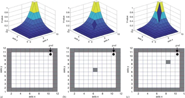
how a change in one state can structurally affect the value function shape.

Comparing the environment sketched in Fig. 2a with those described in Figs. 2b and c one can see that the differences consist only in one obstacle state. Even though, such a single change, from a free state to a state occupied by an obstacle, affected the value function of the states around the obstacle, evidencing the structural dependency of those states with the changed state. Thus, to discover this set of states, from now onwards denoted as the

influence zoneofst,T(st), which has their values computed

by Eq. (2), one can use topological neighborhood in the input space S constructed through a topological map. Topological maps can represent structural and temporal dependencies between states in SCR n_, _nX1, through its

connectivity information that encodes relationships of similarity in the input space.

policy

s_t

s_t-n s_t-n+₁ s_t-n+₂ s_t-n+₃

...

rt-n+1 rt-n+2 rt-n+3 rt-n+4 rt

Fig. 1. State transitions for an RL agent with policy p. White circles represent states in time sequence, and dark circles represent close states that are not visited in sequence (based on[23]).

1 0.8 0.6 0.4 V -v alue 0.2 0 10 axis y axis x 12 11 10 9 8 7 6 5 4 3 2 1

2 4 6 8 10 12

axis y axis x 12 11 10 9 8 7 6 5 4 3 2 1

2 4 6 8 10 12

axis y axis x 12 11 10 9 8 7 6 5 4 3 2 1

2 4 6 8 10 12

1 0.8 0.6 0.4 V -v alue 0.2 0 10 1 0.8 0.6 0.4 V -v alue 0.2 0 10 5 axis y 0 0 5 axis y 0 0 5 axis y 0 0 goal goal goal

(a) (b) (c)

5 axis x 10 5 axis x 10 5 axis x 10

(4)

The topological map capability of representing an input space in R n _{[4,5,11,13,14]} _{is particularly important to}

extend the application of inﬂuence zone concept to

n-dimensional RL problems (n4_{2). However, in order to}

label an algorithm derived from the influence zone concept as recommendable to improve RL efficiency, two targets must be reached: (i) this strategy should reach a performance, in the value function estimations, at least close to eligibility traces [21,25,32] and (ii) the influence zone should execute less updatings than the considered RL models, by restricting the updatings to subsets ofS (as in

[22,30]).

The determination of T(st) considers the following

points: (i) two adjacent spatial states have a tendency to be also adjacent in the value space, this was stated by McCallum [16], who argued that in some sense an RL algorithm basically learns a mapping (V: S-R or Q: S,

A-R) that preserves the topology; and (ii) Since states in

the inﬂuence zone of stare taken to the current state by a

greedy policy, their values should be smaller than the current state value,8s2TðstÞ;VðsÞoVðstÞ. The ﬁrst point

is common to other RL and SOM combinations

[3,7,18,27,30], whereas the second point reduces the number of updatings. As an example, the TRLA [3], an initial version of the algorithm described in Section 5, updates the value function estimate along all topological neighborhoods. However, given st, the inﬂuence zone

updates only those states that satisfy 8s2TðstÞ;

VðsÞoVðs_tÞ. An algorithm to use inﬂuence zone to estimate the value function is described in Section 5; however, the adopted map for the simulations performed is shown next.

4. The instantaneous topological map

Kohonen proposed the SOM consisting of an array ofM

neurons, in which each particular node n has a weight vector wn A S associated to it, and it is linked to other

nodes through established connections. For being pre-determined, the edges of SOM may impair learn of the topological structure of the stimuli space which is initially unknown. Moreover, pre-determined connections can distort the information of complex environments contain-ing obstacles of unknown shape and position.

Two very representative endeavors to construct more accurate topological maps include the works of Martinetz and Schulten [14] and the one proposed by Fritzke[4,5]. Martinetz and Schulten proposed a competitive Hebbian learning model in which learning considers the creation of connections between nodes. This kind of learning employs a winner-take-all method to create a new edge between the two nearest nodes that respond to a given stimulusnA_S_.

Fritzke improved the topology representing networks by proposing a mechanism to include and delete nodes in the topological map allowing the topological map to adapt itself to slow changing topologies.

The instantaneous topological map (ITM)[8]is a more recent model that preserves the ability to insert and exclude nodes, and builds an accurate description of an environment. Such ﬂexibility is obtained through a technique very used in graphics computing for object and environment description: the Delaunay triangulation [6]. Furthermore, the ITM is a fast-learning method, poten-tially suitable to on-line applications. As proposed in[8], the ITM employs Delaunay triangulations regarding the positions of nodes and edges. The ITM can be described as follows:

1.Determination of the first and second winner: considering a stimulusnprovided by the environment, determine the nearest and the second-nearest nodes, n and s, respec-tively,

n¼arg min

i

nwi

; s¼arg min

j;jan

nwj

, (3)

wherei,j, nandsAM.

2.Updating of the weight vectors: for the winner node n, update the components of the weight vector towards the stimulus nconsidering a learning step A:

D_w_n _{¼2 ð}_n_w_n_Þ_. ₍₄₎

3.Creations and deletions of connections and exclusion of disconnected nodes: considering the ﬁrst and the second winner, link them through an edge ns, provided that it does not exist. After such an edge creation, the presence of non-Delaunay edges must be avoided. Hence, for each node m A N(n), where N(n) is the set nodes

connected to n. Find any non-Delaunay edge nm

determined by the criterion (5), and removenm.

8m2NðnÞ:Ifðw_nw_sÞ ðw_mw_sÞo0, (5)

where ws, wn andwm are the weight vectors associated

with nodess,nandm. If any edge is deleted, exclude any remaining node with links.

4.Creation and deletion of nodes due to necessity of accuracy: If the stimulusnsatisﬁes the following criteria:

ðwnnÞ ðwsnÞ40 and wnn

4emax, (6)

whereemaxis a given distance, then insert a new nodey,

with wy¼n, and connected with n by a new valid

Delaunay edgeny. On the other hand, if

wnws

k ko0

:5emax, (7)

remove node s.

(5)

5. The influence zone algorithm

Despite similarities with some SOM-based RL agents like [3,25,29], the concept of influence zone proposed in Section 3 aims to select states, or action–state pairs, in a topological neighborhood to have their values updated.

Thus, similarly to the TRLA [3], some attributes are included in each node of the topological map to establish the topological neighborhoods, and to store the estimate of the value function (VandQ). All attributes are described in

Fig. 3. Two new attributes (Qandr) are added to the four original attributes used in TRLA (w, edges, V, and e), to implement the algorithm of Fig. 4. The attribute Q is a vector in which each element is associated with a neighbor node. The selection of which nodes will have theirQandV

attributes updated follows the satisfaction ofVðsÞoVðs_tÞ, where stis the current state. Differently from the TRLA

algorithm[3], where the value function is only updated in the occurrence of a feedback signal (reward) and all states in a topological neighborhood have their values updated, the inﬂuence zone algorithm is an incremental version of TRLA, characterized through:

(i) Depending on the Error_TD, rðstþ1Þ þgVðstþ1Þ

Qðs;ass_t_þ1Þ, the new algorithm performs an one-step or

an n-step updating in the value function (see Fig. 4). The current strategy starts the value function updating in less iterations since it depends on both the error and the goal occurrence.

(ii) When a n-step updating of the value function occurs, the new algorithm (Fig. 4) deﬁnes the inﬂuence zone of the current state st, T(st), and only the states in T(st)

have their values updated.

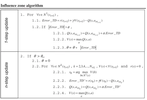
Fig. 4 describes theinfluence zone algorithmin two levels:

Level 1: Updating of a value function at each state transition whenever the Error_TD overcomes a thresh-oldfand such a change, similarly to[30], is limited to one transition (one-step update) of the topological neighborhood.

Level2: In order to reduce the number of updatings, it is triggered only when the error accumulator, y, is higher than a given thresholdy0. In this level occurs ann-step

updating in the computed influence zone followed by a reset operation for the error accumulator (Line 2.1), thus when the loop in Line 2.2 is concluded and the algorithm returns to Level1. Line 2.2 of the algorithm summarizes how the influence zone is considered: given a statest+1, the states belonged to influence zone ofst+1

Influence zone algorithm

1. For ∀s∈N1(st+1),

1.1. _ ( ) ( ) (, )

1 1

1 + − +

=rst+ V st+ Qsasst TD

Error γ

1.2. If Error_TD>φ,

1.2.1.Qsa Qsa Error TD

t

t ss

ss ) (, ) . _ ,

(

1 1 = + +α +

1.2.2.V(s) maxQ(s,a) a

=

1.2.3.θ = θ+ Error_TD

2. If θ > θo,

2.1.θ = 0

2.2. For ∀s∈Nk(st₊₁),k=2,3,4,...,Nviz,V(s)<V(st+1) and r(s)=0,

2.2.1. arg max ( )

) ( 1 Vb

s

s N b b

∈

=

2.2.2. _ '' ( ) ( ) (, )

b ss b b V s Qsa s

r TD

Error = +γ −

2.2.3. Q(s,a ) Q(s,a ) .Error_TD'' b

b ss

ss = +α

2.2.4. V(s) maxQ(s,a) a

=

n

-step update

1

-step update

Fig. 4. The two levels of inﬂuence zone algorithm.

Attributes Description of the attribute Type of data

W reference vector contents vector

edges list of neighbor nodes vector V max value function associated to state w scalar Q state-action value function associated to state wand each edge vector

r return signal when in statew scalar

e indicates if this node is in the current considered topological neighborhood binary

(6)

are found among the k topological neighborhoods of

st+1, Nkðstþ1Þ, and must satisfy the condition

VðsÞoVðs_t_þ₁Þ (Section 3). The ITM is used to learn

Nk_ð_s tþ1Þ.

Identically to the TRLA, for all states in a Voronoi cell2 ([13,14]) of the topological map, the action selection of the

influence zone algorithm aims to reach the neighbor node with the highest value function3(V attribute). There is a ﬁxed number of possible actions represented by vectors (n3, wheren is the input space dimension, and there are three possible values for each element of the vectors associated

with the actions:1, 0, 1) at each Voronoi cell/node and, since the topological map could be an irregular structure. The policypchooses the action that takes the agent to the closest position to the neighbor node with highest V

attribute. This is done by ﬁrst computing the vector vd

which comes from the current node,s, to the weight vector associated with the neighbor node with the highest value function,wgreedy, through the following expression:

vd ¼wgreedys; (8)

the action is selected computing which vector associated with an action is the closest one tovd. This is achieved by

ﬁnding the action-vector which has the max scalar product withvd:

pðsÞ ¼arg max

i2AðsÞ

vdvi

f g, (9)

goal

1

0 0.5

40

35

30

25

20

15

10

5

0 0

10

20

30

40 1

0 0.5

40

35

30

25

20

15

10

5

0 0

10

20

30

40

1

0 0.5

40

35

30

25

20

15

10

5

0 0

10

20

30

40 1

0 0.5

40

35

30

25

20

15

10

5

0 0

10

20

30

40

(E1)

goal goal

(E3) (E4)

goal

(E2)

Fig. 5. Different conﬁgurations used to test the inﬂuence zone algorithm.

2

All states in a Voronoi cell are represented by a node in the topological map.

3

(7)

where A(s) is the set of all possible actions from state s,

vectors vi are associated with each action i from A(s)

representing the expected state transition.

6. Experiments and results

The inﬂuence zone algorithm was tested to solve a complex kind of task: autonomous navigation problem in an initially unknown world [3,17]. This problem comprises an agent that has to move within its environment, avoiding obstacles, to reach an initially unknown goal state. The navigation problem is an instance of a goal-directed RL problem (GDRLP) [12] in which an agent aims to learn a path, between an initial state and a goal state, through RL strategies. Following the initial learning, such a path can be changed to improve the initial solution, to obtain an optimal, or sub-optimal, policy.

All following experiments were simulated, using routines developed by the authors in the MATLABs. For this 2-D navigation problem, eight possible actions for the RL agent were considered. They are represented by the following vectors: v1¼(1,1); v2¼(0,1); v3¼(1,1); v4¼(1,0);

v5¼(1,1);v6¼(0,1);v7¼(1,1); v8¼(0,1)

Four environment conﬁgurations were considered to simulate different levels of complexity for the navigation Q(0)-learning

Environment E1

trials trials

6000

5000

4000

3000

2000

1000

2000 4000 6000 8000 10000 12000 0

0 10 20 30 40 50 60 70 80 90 100 0 10 20 30 40 50 60 70 80 90 100 1000

2000 3000 4000 5000 6000 7000 8000 9000 10000

0

Environment E2

n

umber of steps

n

umber of steps

Environment E1

trials trials

0

0 10 20 30 40 50 60 70 80 90 100 0 10 20 30 40 50 60 70 80 90 100 1000

2000 3000 4000 5000 6000 7000 8000 9000 10000

0

Environment E2

n

umber of steps

n

umber of steps

SARSA(0) Q(λ)-learning SARSA(λ) fast Q(λ) Dyna-Q (N=100) TRLA Influence Zone

Fig. 6. Average number of steps, connecting initial and ﬁnal points, in each trial, in environments ofFig. 5for the eight RL algorithms.

Table 1

ANOVA tables for data presented inFig. 6(level of signiﬁcance 0.05)

Source SS Df MS F p-value

E1 Columns 198098.7 5 39619.7 42.19 0 Error 445077.8 474 939

Total 643176.5 479

E2 Columns 331312.8 5 66262.6 52.85 0 Error 594254.3 474 1253.7

Total 925567.1 479

E3 Columns 135521.2 5 27104.2 32.02 0 Error 401178.8 474 846.4

Total 536700 479

E4 Columns 110658.6 5 22131.7 30.9 0 Error 339457.8 474 716.2

(8)

tasks (Fig. 5). An environment may have three kinds of states: (i) free states are those the agent can visit; (ii)

obstacle statesare prohibited positions of the environment for the agent and (iii) the goal state is the state to be reached by the agent.

The performance of the inﬂuence zone algorithm for autonomous navigation is tested and the results are compared with those obtained with 7 RL algorithms (see Appendix A for the parameters of each algorithm): (i)Q -learning[31]; (ii) SARSA [25]; (iii)Q(l)-learning [21]; (iv) SARSA(l) [25]; (v) Dyna-Q [28]; (vi) fast Q(l)-learning

[32]; and (vii) TRLA [3]. The reward function [29] of the Environment E1

300

250

200

V

alues

V

alues

V

alues

150

100

50

V

alues

100 150 200 250 300 350 400

50

100 150 200 250 300

50

1 2 3 4 5 6 1 2 3 4 5 6

100 150 200 250 300 350 400

50

1 2 3 4 5 6 1 2 3 4 5 6

Group Numbers

Group Numbers Environment E3

Environment E2

Environment E4

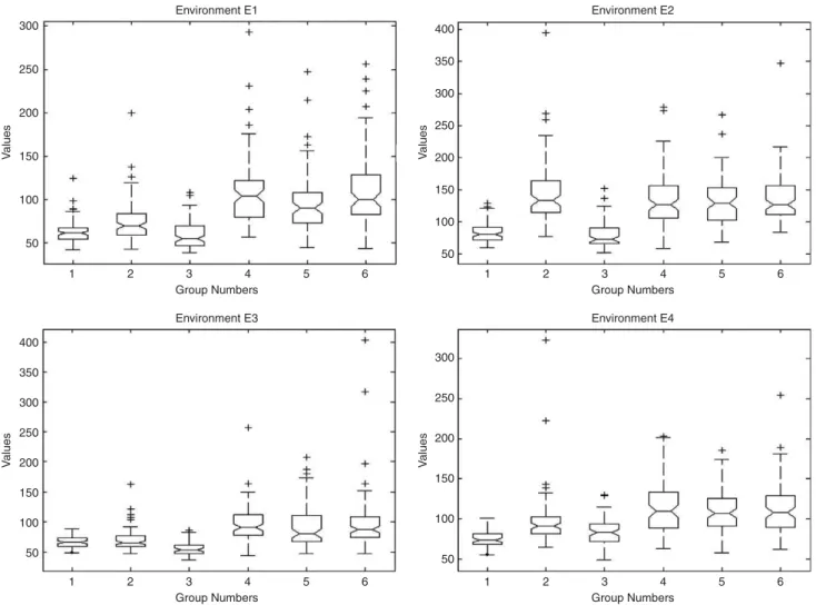
Fig. 7. Notched box plots of trajectory length generated by the six considered algorithms/groups for the four environments. The algorithms are identiﬁed as Group 1—inﬂuence zone algorithm; Group 2—TRLA; Group 3—Dyna-Q; Group 4—fast Q(l)-learning; Group 5—Q(l)-learning; Group 6— SARSA(l).

Table 2

Estimated difference in groups means with a 95% conﬁdence interval

Groups Environments

E1 E2 E3 E4

1 2 [24.9;11.2; 2.6] [77.7;61.7;45.8] [17.2;4.1; 9.0] [34.2;22.1;10.0]

1 3 [9.6; 4.2; 17.9] [12.1; 3.9; 19.9] [1.5; 11.6; 24.7] [19.7;7.6; 4.4]

Table 3

Average number of updatings for the last 50 trials of the results inFig. 6

Environments

E1 E2 E3 E4

Q-learning 3136.3 5055.8 4825.9 4987.2

SARSA 2304.2 4460.6 1143.4 2319.1

Q(l) 4619.8 6419.7 4347.5 4816.6

SARSA(l) 1907.0 2482.1 1768.2 2016.6

FastQ(l) 849.6 1207.2 787.5 883.6

Dyna-Q 5678.1 7282.3 5510.6 6215.4

TRLA 826.0 826.5 561.8 652.7

(9)

RL agents is

rtþ1¼

1 ifstþ1is the goal state;

0 otherwise:

(10)

Two performance criteria were used to compare the RL algorithms. The Criterion 1 (C1) considers the length (number of steps) of the trajectory from a given point to the goal in each trial. The Criterion 2 (C2) computes the total number of value function updatings in each trial.4

6.1. Criterion 1 (C1)

Fig. 6shows the learning performance of each RL agent as function of the trials by showing the number of steps of the generated trajectories.

The data sketched inFig. 6represents the average of 80 experiments for each environment. From such curves, there is a clear difference between the trajectories generated by

Q-learning and SARSA, and the trajectories generated by other RL algorithms. Hence, the performance of the inﬂuence zone algorithm is analyzed only in comparison with the TRLA, Dyna-Q, fast Q(l)-learning, Q(l) and SARSA(l). For a statistical analysis of such data, ANOVA and the extended Tukey test [15,19,26] were carried out. The purpose of one-way analysis of variance (ANOVA) is to verify whether data from several groups have a common mean. That is, in the current case, to determine whether the algorithms are actually different, according to the C1. The

null hypothesisin ANOVA is that all means are equal; this hypothesis is rejected if the p-value [15,19,26] has a very small value. Table 1 shows thep-values computed in the ANOVA table for each environment.

Allp-values inTable 1are null, then at least one of those algorithms generated trajectories with a different mean from the other ones.

The notched box plots (Fig. 7) allow to identify two clusters: (i) Groups 1-3 (Inﬂuence Zone, TRLA and

Dyna-Q), having shorter trajectories than (ii) Groups 4–6 (fast

Q(l)-learning, Q(l)-learning, SARSA(l)). However, to specify with a level of significance which algorithms are similar, and which ones have the smallest trajectories, a multiple comparison test is necessary. In this case, the Tukey’s significant-difference (TSD) test [15,19,26] was used. The Turkey test is the equivalent oft-test for multiple comparisons and consists in the computation of confidence intervals for the means of a pair of groups. If the value 0 (zero) is not within the computed interval then the means are different.Table 2presents the 95% confidence interval for the estimated difference in means of the Groups 1–3, the short-trajectory cluster inFig. 7.

The three values associated with each environment include the (i) lower limit; (ii) the estimated mean, and (iii) the upper limit of the difference between data from the groups being compared. Hence, if an interval contains 0 (zero), then the two groups under comparison are not considered different. Based on the interval contents, the means of trajectory lengths generated by inﬂuence zone algorithm and Dyna-Q are not statistically different (marked row in Table 2). Furthermore, these two algorithms produced the shortest trajectories.

6.2. Criterion 2 (C2)

The procedure adopted to analyze the performance of the considered RL algorithms for C1 is followed in this subsection for C2. Then, the data was collected in 80 experiments (100 trials each) for each algorithm in the four considered environments.

Table 3 summarizes the average number of value

function updatings performed by each algorithm, and these data is used to indicate the candidates to the best performance according to C2. Table 3shows Q-learning, SARSA, Dyna-Q, SARSA(l) andQ(l)-learning exhibit an undesirable behavior: they do execute a high number of updating in all four environments.

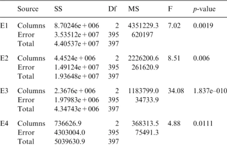
Hence, the performance of the influence zone algorithm is compared with the algorithms that presented lower number of updatings: TRLA and fast Q(l)-learning. ANOVA, used inTable 4, shows the existence of significant differences between the means of the number of updatings with very small values for p-value. As a hypothesis test, ANOVA adopted a level of significance (a-level), equal to 0.05 in the current case. Then (since p-valueo0.05) there is, at least, one of the RL algorithms (Influence Zone, TRLA or fastQ(l)-learning) statistically distinct. In order to find statistical differences among the tested algorithms, the notched box plots shown inFig. 8shows the medians of updatings for the three considered models. These graphs suggest that the TRLA and the fastQ(l)-learning have the Table 4

ANOVA tables for data summarized inTable 3(level of signiﬁcance 0.05)

E1 Columns 8.70246e+006 2 4351229.3 7.02 0.0019 Error 3.53512e+007 395 620197

Total 4.40537e+007 397

E2 Columns 4.4524e+006 2 2226200.6 8.51 0.006 Error 1.49124e+007 395 261620.9

Total 1.93648e+007 397

E3 Columns 2.3676e+006 2 1183799.0 34.08 1.837e–010 Error 1.97983e+006 395 34733.9

Total 4.34743e+006 397

E4 Columns 736626.9 2 368313.5 4.88 0.0111 Error 4303004.0 395 75491.3

Total 5039630.9 397

4

(10)

lowest number of updatings in environments E1 and E2, and that the inﬂuence zone algorithm has the lowest number of updatings in environments E3 and E4.

Tables 5 and 6show the conﬁdence intervals computed by the Tukey test to validate the above initial hypothesis about the performance of the inﬂuence zone algorithm in

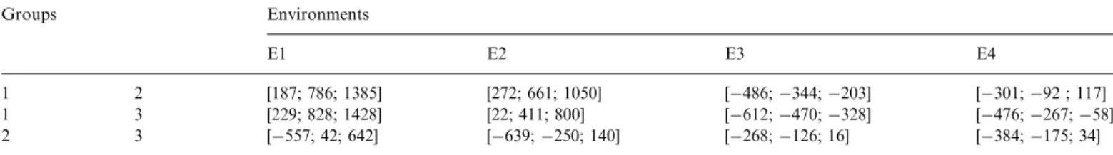
comparison with the TRLA and the fastQ(l)-learning in their number of value function updatings.Table 5 points out that the inﬂuence zone algorithm has different number of updating in all cases, except for the TRLA in E4, whereas the TRLA and the fast Q(l)-learning have the same performance. Table 5 together with Fig. 8 suggests Table 5

Estimated difference in groups means with a 95% conﬁdence interval

Groups Environments

E1 E2 E3 E4

1 2 [187; 786; 1385] [272; 661; 1050] [486;344;203] [301;92 ; 117]

1 3 [229; 828; 1428] [22; 411; 800] [612;470;328] [476;267;58]

2 3 [557; 42; 642] [639;250; 140] [268;126; 16] [384;175; 34]

Environment E1

Group Numbers 5000

4500

4000

3500

3000

2500

2000

1500

1000

500

0

1000

200 600 600 800

1000 1500 2000 2500 3000 3500

500

0

1000 1200 1400 1600

200 400 600 800

0

1 2 3 1 2 3

V

alues

V

a

lues

V

alues

V

alues

Environment E2

Group Numbers

Environment E3

Group Numbers

Environment E4

Group Numbers

(11)

that the inﬂuence zone algorithm has better performance in more complex environments (E3 and E4).

6.3. Change in environment structure

The four room conﬁguration ofFig. 9were used to test the RL agents performance in a changeable environment in which the reward function[29]is given as follows:

rtþ1¼

þ1 ifstþ1is the goal state; 1 ifstþ1is an obstacle;

0 otherwise: 8

> <

> :

(11)

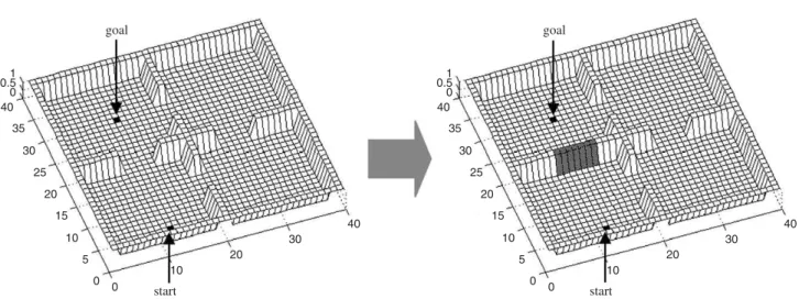
To verify the comparative behavior of the influence zone approach to respond to modifications in the four rooms, 30 experiments were executed for each algorithm in the environment of Fig. 9 where the rooms have all internal doors open during the first 99 trials, and a closed door from trial 100 to trial 200. This closed door blocks the shortest path between initial and goal states, then a new trajectory should be learned. In the first stage (trials 1–99): the influence zone algorithm, Dyna-Q, fastQ(l)-learning,

Q(l)-learning and SARSA(l) approaches generated a cluster of shortest trajectories (in average, 28.83; 37.53; 39.04; 43.60 and 41.74, respectively), whereas the one-step algorithms, Q-learning and SARSA, generated the worst results (in average, 89.71 and 83.78, respectively). In this experiment, the TRLA was not considered since its original work [3]does not consider a multi-reward function as in the expression (11).

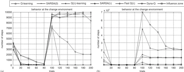
Fig. 10 shows the behavior of the simulated algorithms for the criteria C1 (Fig. 10a) and C2 (Fig. 10b). The comparative behaviors during trials 1–99 are very similar, for both criteria, to those reported in Sections 6.1 and 6.2. Hence, the behaviors after the change in environment topology are the focus of this subsection.

FromFig. 10a, it is clear the difficulty of most of the RL algorithms to learn new trajectories in the presence of the new obstacle. In this second stage, only the influence zone and the Dyna-Qeffectively adapt themselves reaching the target, not expressing a tendency to maintain the trajec-tories learned in first stage. Even though, the superiority of the influence zone algorithm against Dyna-Q is easily detectable, in terms of numbers of steps, the first one produced trajectories within the range [55.8976.71] at trial 200, while Dyna-Qgenerated trajectories within the range [2043.074046.6] at the same trial.

The Dyna-Q employed its model of the world, i.e., learning a new value function involves random selection of states in which the agent avoids the closed door in the environment, causing slow convergence to the new value function (in average, 339860.0 value function updatings, for the last 50 trials). The influence zone update strategy is more efficient because of the topological map: after closing the door, the influence zone restricts the updating of the value function to the set of states reaching the closed door. Thus, a lower number of states had their values updated: 525.39 value function updatings, in average, for the 50 last trials.

Fig. 10b also showsQ-learning and SARSA compute a small number of value function updatings.

Thep-value ofTable 5is evidence that the three means of the inﬂuence zone algorithm, Q-learning and SARSA are not the same. This is also shown inFig. 11, where it is easy to see such differences.

The average number of updatings with influence zone is 356.1, while Q-learning and SARSA performs 8381.0 and 10000.0, respectively. The presented results show a remarkable flexibility of the influence zone algorithm.

goal

1 0.5 0 40

35

30

25

20

15

10

5

0 0

10

20

30

40

1 0.5 0 40

35

30

25

20

15

10

5

0 0

10

20

30

40

start

goal

start

Fig. 9. Experimental sketch for analysis of the performance of RL models in the environment with change in the topology. Table 6

ANOVA tables for data presented inFig. 10b(level of signiﬁcance 0.05)

Columns 1.64385e+009 2 8.21927e+008 235.49 0 Error 3.03651e+008 87 3.49025e+006

(12)

7. Conclusions

The main contribution of this work is to propose an efficient strategy to accelerate RL by adopting the concept of influence zone to update the value function. Differently from the TRLA[3], that as influence zone algorithm uses a topological map to update the value function, the current algorithm is an improvement capable to work with more complex reward functions as the expression (11) since this strategy permits to restrict the updatings only to the set of states that have their value correlated with the value of the current state. Such a concept allows choosing a number of

states to have their values updated at each state transition. The learned value function is an estimation of the optimal value function (Section 6), at the explored area of the environment, where states in the same topological neighbor-hood are considered as having a similar value function. This hypothesis is consistent with the temporal credit assignment performed by standard RL algorithms since states in the same topological neighborhood of a goal state might have a similar number of state transitions to reach such a goal.

The obtained results assessed the efficiency of the proposed value function update strategy. This simple mechanism allows similar or better learning acceleration than that observed in RL algorithms as the Dyna-Qand the fast Q(l)-learning (Section 6). Such a performance suggests that the proposed algorithm is eligible to be applied in on-line problems since it reduced significantly the trajectory length since the first trial.

In order to label an algorithm as recommendable to improve RL efficiency, two performance criteria are considered: (i) the capacity to reach near optimal solution (in our case, the trajectories) in few trials, and (ii) the necessity of reduced number of updatings to diminish computing time. Section 6.1 shows the means of trajectory lengths generated by influence zone algorithm are not statistically different from the Dyna-Q, overcoming the other six RL-simulated algorithms. Furthermore, these results suggest an improvement of the influence zone algorithm in comparison with the TRLA. The influence zone algorithm is clustered with the TRLA and the fast

Q(l)-learning as those with less updatings. The results suggest that the proposed model tends to do better than the other two in more complex environments (Section 6.2).

Remarkable distinct performances were observed when the environment conﬁguration changed (Section 6.3). In RL agents, performance degradation can occur due to environ-ment changes when the policy can become unsuitable to such a Q-learning SARSA(0) Q(λ)-learning

behavior at the change environment 10000

n

umber of steps

n

umber of steps

9000

8000

7000

6000

5000

4000

3000

2000

1000 1

2 3 4 5 6 7

0

0 20 40 60 80 100 120 trials

(a) (b)

140 160 180 200 20 40 60 80 100 120 trials

140 160 180 200 behavior at the change environment

x 105

SARSA(λ) Fast Q(λ) Dyna-Q Influence zone

Fig. 10. (a) Number of steps, connecting initial and ﬁnal points, in each trial, in the four room environment, (b) Number of value function updates, in each trial, during the training.

Number of updatings in the Changable Environment

Group Numbers 1

10000

9000

8000

7000

6000

5000

4000

3000

2000

1000

0

V

alues

2 3

(13)

new condition. Sutton and Barto (Chapter 9 in[29]) see this general problem as a version of the exploration–exploitation conflict: the agent must explore the environment to learn its changes, without disrupting the invariant knowledge pre-viously acquired. The results plotted inFig. 10, and discussed in Section 6.3, suggest the influence zone as a possible heuristic to reduce this conflict with a practical strategy: the prior knowledge represented by the topological map is used to determine the states affected by the changes, and only their values are updated.

Despite its promising first results, the influence zone implementation is very dependent on how precise is the environment topological representation by the SOM, and the algorithm can be improved by adopting more efficient search strategies to determine the topological neighborhoods. Inadequate connections between nodes or inaccurate repre-sentation of the goal state can deteriorate its performance. The potential of the proposed algorithm suggests future works with problems in dimensions higher than two. A 3D problem as in[11]could be an interesting test for the influence zone algorithm. Besides, the authors hope to investigate the applications of the current algorithm and its future variations to partially observable problems[9], a very active field in RL.

Acknowledgments

The authors would like to thank Dr. Jeremy Wyatt, University of Birmingham, UK, for his help regarding the experiments in the changeable environment (Section 6.3). This work was supported by FAPESP Grant No. 98/ 12700-5.

Appendix A

Algorithms’ parameters used in simulations are shown in

Table A.1.

References

[1] R. Bellman, Dynamic Programming, Princeton University Press, Princeton, NJ, 1957.

[2] D.P. Bertsekas, J.N. Tsitsiklis, Neuro-Dynamic Programming, Athena Scientiﬁc, Belmont, MA, 1996.

[3] A.P.S. Braga, A.F.R. Arau´jo, A topological reinforcement learning agent for navigation, Neural Comput. Appl. 12 (3-4) (2003) 220–236. [4] B. Fritzke, A growing neural gas network learns topologies, Adv.

Neural Inform. Process. Syst. 7 (1995) 625–632.

[5] B. Fritzke, Unsupervised ontogenetic networks, in: E. Fiesler, R. Beale (Eds.), Handbook of Neural Computation, Institute of Physics Publishing and Oxford University Press, 1996.

[6] P.L. George, Automatic Mesh Generation—Application to Finite Element Methods, Wiley, New York, 1991.

[7] A. GroX_{mann, Continual learning for mobile robots, Ph.D. thesis,}

School of Computer Science, The University of Birmingham, Birmingham, UK, 2001.

[8] J. Jockusch, H. Ritter, An instantaneous topological mapping model for correlated stimuli. Proceedings of the IJCNN’99, 1999, pp. 445. [9] L.P. Kaelbling, M.L. Littman, A.W. Moore, Reinforcement learning:

a survey, J. Artif. Intell. Res. 4 (1996) 237–285.

[10] M.H. Kalos, P.A. Whhitlock, Monte Carlo Methods, Wiley, New York, 1986.

[11] M.Y. Kim, H. Cho, Three-dimensional map building for mobile robot navigation environments using a self-organizing neural net-work, J. Robot. Syst. 21 (6) (2004) 323–343.

[12] S. Koenig, R.G. Simmons, The effect of representation and knowl-edge on goal-directed exploration with reinforcement learning algorithms, Mach. Learn. 22 (1996) 227–250.

[13] T. Kohonen, Self-Organization and Associative Memory, Springer, Heidelberg, 1984.

[14] T. Martinetz, K. Schulten, Topology representing networks, Neural Networks 7 (3) (1994) 507–522.

[15] R.L. Mason, R.F. Gunst, J.L. Hess, Statistical Design and Analysis of Experiments, Wiley, New York, 1989.

[16] R.A. McCallum, Using transitional proximity for faster reinforce-ment learning, Proceedings of the Ninth International Conference on Machine Learning, 1992, pp. 316–321.

[17] J. Mila´n, R. del, Rapid, safe, and incremental learning of navigation strategies, IEEE Trans. Syst., Man, Cybernet. 26 (1996) 408–420. [18] J. Milla´n, R. del, D. Posenato, E. Dedieu, Continuous-action

Q-learning, Mach. Learn. 49 (2002) 247–265.

[19] D.C. Montgomery, Design and Analysis of Experiments, Wiley, New York, 1984.

[20] A.W. Moore, C.G. Atkeson, Prioritized sweeping: reinforcement learning with less data and less time, Mach. Learn. 13 (1993) 103–130. [21] J. Peng, R.J. Williams, Incremental multi-step Q-learning, Mach.

Learn. 22 (1996) 283–290.

[22] C.H.C. Ribeiro, Aspects of the behaviour of a learning agent in control tasks, Ph.D. thesis, Imperial College of Science, Technology and Medicine, University of London, 1998.

[23] C.H.C. Ribeiro, Reinforcement learning agents, Artif. Intell. Rev. 17 (2002) 223–250.

[24] H. Ritter, T. Martinetz, K. Schulten, Neural Computation and Self-Organizing Maps—An Introduction, Addison-Wesley Publishing Company, Reading, MA, 1992.

[25] G.A. Rummery, Problem solving with reinforcement learning, Ph.D. thesis, Cambridge University, 1995.

[26] W.C. Scheﬂer, Statistics—Concepts and Applications, The Benjamin/ Cummings Publishing Company, Inc., 1988.

[27] A.J. Smith, Applications of the self-organising map to reinforcement learning, Neural Networks 15 (8–9) (2002) 1107–1124.

[28] R.S. Sutton, Dyna, an integrated architecture for learning, planning, and reacting, SIGART Bull. 2 (1991) 160–163 ACM Press. [29] R.S. Sutton, A. Barto, Introduction to Reinforcement Learning, MIT

Press/Bradford Books, Cambridge, MA, 1998. Table A.1

Algorithms’ Parameters used in Simulations Algorithms Parameters

Q(0)-learning a¼0.5;g¼0.8;e¼0.3 SARSA(0) a¼0.5;g¼0.8;e¼0.3 Q(l)-learning a¼0.5;g¼0.8;e¼0.3;l¼0.7;

eH¼1016

SARSA(l) a¼0.5;g¼0.8;e¼0.3;l¼0.7;

eH¼10 16

FastQ(l) a¼0.5;g¼0.8;e¼0.3;l¼0.7;

em¼10 16

Dyna-Q a¼0.5;g¼0.8;e¼0.3;N¼100 TRLA g¼0.8;e¼0.3;emax¼0.5;A¼104 Inﬂuence zone a¼0.5;g¼0.8;e¼0.3;emax¼0.5;

A¼104;f¼1016;yo¼0.5

a¼reinforcement learning rate;g¼discount factor;e¼e-greedy policy parameter; l¼lambda; eH¼threshold to control the H list inclusion;

(14)

[30] C. Touzet, Neural reinforcement learning for behaviour synthesis, Robot. Autonom. Syst. 22 (3–4) (1997) 251–281.

[31] C.J.C.H. Watkins, Learning from delayed rewards, Ph.D. thesis, King’s College, Cambridge, 1989.

[32] M. Wiering, J. Schimidhuber, Fast online Q(l), Mach. Learn. 33 (1998) 105–115.

Arthur P.S. Braga received his B.S. degree in Electrical Engineering from Federal University of Ceara´ in 1995. The M.S. and Ph.D. degrees in Electrical Engineering from the University of Sa˜o Paulo in 1998 and 2004, respectively. His Ph.D. thesis concerned a methodology for the learning acceleration of reinforcement learning algo-rithms. His research interests include theory and applications in the areas of reinforcement learn-ing, neural networks and robotics. Currently, Dr. Braga is developing his post-doctorate in the automation of manufacturing processes through artiﬁcial intelligence techniques.