An Optimized Numerical Method for Solving the
Two-Dimensional Impedance Equation
C. M. A. Robles G.
IAENG, Member
, A. Bucio R. and M. P. Ramirez T.
IAENG, Member
.
Abstract—We study an optimized numerical method for solving the forward problem of the two-dimensional Impedance Equation. Based upon elements of the modern Pseudoanalytic Function Theory, its performance is tested employing sinusoidal conductivity functions within the unit circle. Then a collection of experimental data are displayed for illustrating its effectiveness. The work closes with a brief discussion of the contribution to the Electrical Impedance Tomography problem.
Index Terms—Computational method, Electrical Impedance Equation, Pseudoanalytic Function Theory.
I. INTRODUCTION
T
HE elements of the modern Pseudoanalytic Function Theory [7], have been successfully applied for sorting out the forward problem of the Impedance Equation in the planediv(σgradu) = 0, (1) where σ is the conductivity and u is the electric poten-tial. Specifically, when σ can be expressed as a separable-variables function, it is possible to approach the general solution of (1) in asymptotic form, harnessing Taylor series in formal powers [2].
Nevertheless, the application of this technique may have some restrictions when dealing with engineering problems, because the conductivity functions rising from experimental models, in general, do not posses a separable-variables structure. An alternative for overpassing this restriction was posed in [9], where it was shown that, under certain circum-stances, every physical-rising conductivity distribution, can be considered a limit case of a piecewise separable-variables function.
The relevance of efficiently solving the forward problem for (1), if we are to solve the Electrical Impedance Tomog-raphy problem (also called inverse problem), was widely exposed in a variety of works, among which [12] is one of the most important. In this sense, the results posed in [8], and subsequently rediscovered in [1], are indeed very significant, because they allowed to sift out the rink for approaching the general solution of the Impedance Equation in the plane.
After publishing these works, many interesting papers, dedicated to numerically solving the Dirichlet boundary value problem of (1) in the plain, have achieved to approach the solutions with considerable accuracy (see e.g. [6]).
The main contribution of this work is to propose an efficient numerical method, whose algorithm displays an ad-equate valance between the computational cost and accuracy.
C. M. A. Robles G.is with the National Polytechnique Institute, ESIME C. Mexico, cesar.robles@lasallistas.org.mx
A. Bucio R. is with the National Polytechnique Institute, UPIITA, Mexico, ari.bucio@gmail.com
M. P. Ramirez T. is with the Communications and Digital Signal Processing Group, Engineering Faculty of La Salle University, Mexico, marco.ramirez@lasallistas.org.mx.
We shall remark once more that many of the existing methods are highly accurate, but they engross the usage of computa-tional resources, and also impose mathematical restrictions that locate them far away from engineering applications. The method posed in the following paragraphs may avoid these problems, becoming appropriate for, e.g., analysing Electrical Impedance Tomography problems upcoming from clinical cases.
Hence, we first broach a simplified numerical method for solving (1) at the boundary of some domain in the plain [3]. This is done by approaching elements of a complete set of solutions for a Vekua equation [11], fully equivalent to (1). Then we examine a special class of examples, in order to illustrate the effectiveness of the method, lodging an expla-nation of its performance through a set of control parameters. The conclusions contain the arguments that might justify the viability of employing this new technique.
II. PRELIMINARIES
According to the Pseudoanalytic Function Theory posed in [2], let us consider a pair of complex-valued functions
(F, G)that fulfil the condition Im F G
>0, (2)
whereF denotes the complex conjugate ofF:
F=ReF−iImF.
Thus, any complex function W can be expressed by the linear combination ofF andG:
W =φF+ψG,
whereφ andψ are real-valued functions.
A pair (F, G) that heeds (2) is named a generating pair. This concept allowed L. Bers to introduce the(F, G) -derivative of a functionW:
∂(F,G)W = (∂zφ)F+ (∂zψ)G, (3) where ∂z = ∂x∂ −i∂y∂ , and i2 = −1. This derivative will only exist if
(∂zφ)F+ (∂zψ)G= 0, (4) where∂z= ∂x∂ +i∂y∂ .
Moreover, when introducing the notations
A(F,G)=
F ∂zG−G∂zF
F G−F G , B(F,G)=
F ∂zG−G∂zF
F G−F G ,
a(F,G)=
G∂zF−F ∂zG
F G−F G , b(F,G)=
F ∂zG−G∂zF
F G−F G ; (5)
the equation (3) can be written as
forasmuch (4) attains
∂zW −a(F,G)W −b(F,G)W = 0. (7) Concretely, the notations (5) are called thecharacteristic coefficientsof the generating pair(F, G). The expression (6) is referred as the(F, G)-derivative ofW, and (7) is the Vekua equation [11].
Remark 1: The functions
F =p, G= i
p, (8)
wherepis a non-vanishing real-valued function, within some domainΩ, makes up a Bers generating pair since they satisfy (2), and their characteristic coefficients are:
A(F,G)=a(F,G)= 0,
B(F,G)=−∂zpp, b(F,G)=−∂zpp.
(9)
Definition 1: Let us suppose that (F0, G0) and (F1, G1) are two generating pairs with the form (8), and let their characteristics coefficients (5) fulfil the relations
B(F0,G0)=−b(F1,G1).
Then (F1, G1) will be called a successor pair of(F0, G0), and(F0, G0)will be a predecessorof (F1, G1).
Definition 2: Let us consider a set of generating pairs {(Fn, Gn)}, n= 0,±1,±2, ... such that each (Fn, Gn) is a predecessor of(Fn+1, Gn+1). The set will be then called a generating sequence. If (F, G) = (F0, G0), we say that
(F, G) is embedded into {(Fn, Gn)}. Furthermore, if there exist a number k such that (Fn+k, Gn+k) = (Fn, Gn), we assert that the generating sequence isperiodic, with a period of magnitudek.
Remark 2: Let us consider a generating pair of the form (8). If pis a separable-variables function
p=p1(x)·p2(y), (10) the pair will be embedded into a periodic generating se-quence, with period k= 2, being
Fm=p1(x)p2(y), Gm=
i p1(x)p2(y)
,
when mis even, and
Fm=
p2(y)
p1(x)
, Gm=i
p1(x)
p2(y)
,
when mis odd.
The concept of the(F0, G0)-integral was also introduced by professor L. Bers [2].
Definition 3: The adjoint generating pair (F∗
0, G∗0) corre-sponding to(F0, G0)with the form (8), is defined as:
F0∗=−iF0, G∗0=−iG0. (11)
Definition 4: The (F0, G0)-integral of a complex valued functionW is defined as:
Z z
z0
W d(F0,G0)z=F0Re
Z z
z0
G∗
0W dz+G0Re
Z z
z0
F∗
0W dz. Specifically, since the (F0, G0)-integral of the (F0, G0) -derivative of W reaches
Z z
z0
∂(F0,G0)W d(F0,G0)z=W−φ(z0)F0−ψ(z0)G0, (12)
and considering that [2]
∂(F0,G0)F0=∂(F0,G0)G0= 0,
the integral expression (12) can be considered the(F0, G0)
-antiderivativeof the function∂(F0,G0)W.
We refer the reader to the specialized literature [2] and [7], for a detailed description about the existence of the(F0, G0) -antiderivative. Hereafter, when this concept is evoked, every complex-valued function will be(F0, G0)-integrable by def-inition.
A. Formal Powers
Professor L. Bers [2] generalized the classical result for expanding any analytic function in Taylor series, for the set of the so-called Pseudoanalytic Functions, by midst of what he introduced asformal powers.
Definition 5: The formal powerZm(0)(a0, z0;z)with com-plex constant coefficienta0, center atz0, depending uponz, formal exponent0, and corresponding to the generation pair
(Fm, Gm), is expressed as:
Zm(0)(a0, z0;z) =λmFm+µmGm,
whereλmandµmare real constants, fulfilling the condition
λmFm(z0) +µmGm(z0) =a0.
The higher exponents of the formal powers are defined according the recursive formulas
Zm(n+1+1)(an, z0;z) =
= (n+ 1)Rz
z0Z (n)
m (a0, z0;z)d(Fm,Gm)z.
(13)
Dwell that these integrals operators are indeed(Fm, Gm) -antiderivatives, and every formal power of the set
n
Zm(n)(an, z0;z)
o∞
n=0, is an(Fm, Gm)-pseudoanalytic function [2].
Employing the previous statements, L. Bers proved that any (Fm, Gm)-pseudoanalytic function can be expressed in
Taylor series in formal powers
W =
∞
X
n=0
Zm(n)(an, z0;z); (14)
where
an=
1 n!∂
(n)
(Fm,Gm)W(z0).
In this purport, this is an analytical representation of the general solution for the Vekua equation (7).
B. The two-dimensional Impedance Equation
Let us consider the two-dimensional case of the Impedance Equation (1), and let us suppose that the conductivityσcould be expressed in terms of a separable-variable function:
σ=σ1(x)·σ2(y). Introducing the notations
W =√σ
∂ ∂xu−i
∂ ∂yu
, p=
s σ2(y)
σ1(x)
the Impedance Equation can be written as a Vekua equation
∂zW −
∂zp
p W = 0. (16)
Furthermore, as it was elegantly stated in [5], the set
n
ReZm(n)(1,0;z)|Γ, ReZm(n)(i,0;z)|Γ
o∞
n=0, (17) conforms a complete system for approaching solutions of the Dirichlet forward problem for (1). HereΓrepresents the boundary of the domain Ω, where the formal powers are defined.
In other words, let
u(n)(1,0, z) =ReZm(n)(1,0;z)|Γ,
u(n)(i,0, z) =ReZm(n)(i,0;z)|Γ;
n= 0,1,2, ...
(18)
If a boundary condition u|Γ is provided, we can always approach it asymptotically
lim
N→∞
N
X
n=0
αnu(n)(1,0, z) +βnu(n)(i,0, z)
=u|Γ,
(19) whereαj andβj are real numbers.
This procedure proved its effectiveness in several works (see e.g. [5], [6] and [10]), where the numerical approaches achieved highly accurate results.
Referring the reader to [9], where it was proven that any physical-rising conductivity function, could be considered the limit case of a piece-wise separable-variables function, we will explain the method for numerically approaching a finite set of formal powers with the form (17), in order to solve the forward problem for (1).
III. FORMALPOWERAPPROACHING
Attaching the modern Pseudoanalytic Function Theory studied in [7], to the classical results of [2], we present an improved numerical method that, based onto a previous proposal [3], possesses a higher degree of accuracy and numerical stability. Our explanations will be perform consid-ering the formal powers with coefficients an = 1, because not any important methodological variation takes place when consideringan=i.
Thence, let us consider a collection ofK+ 1 points {r[k]}, k= 0,1, ..., K;
equidistantly located in a closed interval[0,1]. If the interval
[0,1] coincides with a radius R of the unit circle, whose center is z0 = 0, with some specific angle θ ∈[0,2π), we will immediately obtain a collection of points allocated in the plane:
{(x[k], y[k])}, k= 0,1, ...K;
constructed according to the rule
x[k] =r[k] cos(θ); y[k] =r[k] sin(θ).
Thus the formal powers over such radius R can be approached employing the recursive expressions:
Z(n+1)[k] =AF[k]· ·Re
k
X
q=0
G∗[q]Z(n)[q] +G∗[q+ 1]Z(n)[q+ 1]∆z[q]+ +AG[k]·
·Re k
X
q=0
F∗[q]Z(n)[q] +F∗[q+ 1]Z(n)[q+ 1]∆z[q], (20) where
∆z[q] =x[q+ 1]−x[q] +i(y[q+ 1]−y[q]),
andAis a factor that warrants the numerical stability of the method (see [4]). This is, it possesses a direct influence in the convergence and steadiness of the numerical calculations. More precisely, for the examples examined further, we will fix A = 8. The absence of the sub-index m in the formal powers shown above, indicates that they all belong to the same generating pair.
In order to display the mathematical operations in an algorithmic format, it will be convenient to denote the operations described in (20) as
Z(n+1)[k] =BhZ(n)[k]i.
It is clear that this procedure can be performed for a variety of radii {Rs}, s = 1,2, ..., S; each one associated to an angleθs belonging to the set
θ1= 0, θ2=
2π S , θ3=
4π
S , ..., θS =
2(S−1)π S
.
We shall also remark that the numerical method was fully developed inGNU C, employing an AMDR
CPU ATHLON 64-4800R
at 2.50 GHz.
The Algorithm 1 summarizes the programming details for numerically approaching N formal powers, over S number of radii, and consideringK+ 1points per radius.
Algorithm 1Boundary value problem solver
S←1000; (Number of radii)
N←40;(Maximum number of Formal Powers)
K+ 1←1001; (Number of points per radius) whiles= 1→S do
whilen= 1→N do whileq= 0→K do
Z(n+1)[k] =B
Z(n)[k]
; end while
end while end while
functionORTHONORMALIZATION
(Classical Gram-Schmidt Orthonormalization Process) end function
functionAPPROACH BOUNDARY CONDITION;
PN
n=0 αnu(n)(1,0, z) +βnu(n)(i,0, z)
end function
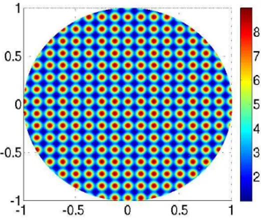
Fig. 1. σ= (2 + cos(2ˆπx)) (2 + sin(2ˆπy)).
Fig. 2. σ= (2 + cos(16ˆπx)) (2 + sin(16ˆπy)).
IV. EXPERIMENTAL ANDRESULTS
According to the statements reported in [10], for bet-ter illustrating the results obtained employing the method summarized in the Algorithm 1, we selected a conductivity functionσ given by a sinusoidal form:
σ= (2 + cos(2τˆπx)) (2 + sin(2τπy))ˆ , τ = 1,8; (21) where
ˆ
π= 3.1416, (22)
since it is not convenient to use a closer approach for the numberπ, as it will be explained further. This case requires a high degree of accuracy when solving the Dirichlet boundary value problems [10]. The Figure 1 displays the conductivity inside the unitary circle whenτ = 1, whereas Figure 2 plots the case whenτ = 8.
As the boundary condition, we shall impose an exact solution of (1):
u= √2
3arctan
1
√
3tan (ˆπx)
+
+√2
3arctan
1
√
3+ 2
√
3tan (ˆπy)
. (23)
corresponding to the case when
σ= (2 + cos(2ˆπx)) (2 + sin(2ˆπy)).
The reason for employing the truncate value (22), is the indetermination of the exact solution (23) when πˆ→π.
Fig. 3. Approach withτ= 8,N= 20,S= 200,K= 200.
It is easy to verify that the exact solution (23) can not be extended for the cases when τ= 2,8. Nonetheless, we will continue using it as the boundary condition, for analysing the remaining conductivity functions, in order to stablish a parameter of comparison for examining the behaviour of the method.
For the numerical approached solution at the boundaryΓ, we will employ the notation
uapp= N
X
n=0
αnu(n)(1,0, z) +βnu(n)(i,0, z)
. (24)
Thus, the absolute error can be introduced as
E = Z 2π
0
(u|Γ−uapp)2dl
1 2
, (25)
where u|Γ is in fact the exact solution (23), valued at the perimeter of the unitary circle, andl∈[0,2π).
We compute a set of examples using the conductivities (21), considering different maximum numbers of formal powersN, radiiS, andK+ 1points per radius, whose main results are displayed in the Tables shown bellow.
In order to provide a basic qualitative illustration of the performance, the Figure 3 plots the approached solution for
τ = 8, N = 20, S = 200, and K = 200; whereas Figure 4 displays the case whenτ = 8, N = 160, S = 1000, and
K= 200.
For the first case, the total error was E ∼ 1.7791; and for the second case we had an error of E ∼ 0.0035. It is remarkable that almost no difference can be appreciated between the curves displayed in Figure 4, corresponding to the approached solution uapp and the boundary condition
u|Γ.
A quantitative perspective is provided in the Tables I and II. The Table I contains the data reached when fixingτ= 2, that, as a matter of fact, corresponds to the case of the Figure 1. Here, it is possible to appreciate that when decreasing the number S of radii, K + 1 points per radius, and N
formal powers, the absolute error E increases, as it could be expected.
Beside, the Table I illustrates that a relatively low number
N of formal powers, can adequately approach the boundary condition u|Γ; whereas the increment of points per radius
Fig. 4. Approach withτ= 8,N= 160,S= 1000,K= 200.
TABLE I
BRIEF RELATION AMONG PARAMETERS OF THE OPTIMIZED METHOD AND THE ABSOLUTE ERRORE
Radii Points Formal Powers Error Time
S K+ 1 N E t(seconds)
1000 1001 40 0.0060 4724.90
1000 1001 35 0.0185 4173.71
1000 1001 30 0.0247 3531.44
1000 1001 25 0.0106 2951.68
1000 1001 20 0.1178 2743.682
800 1001 20 0.1196 3103.35
600 1001 20 0.1427 1507.72
400 1001 20 0.1173 1015.52
200 1001 20 0.0889 481.13
200 801 20 0.0889 308.94
200 601 20 0.0889 180.47
200 401 20 0.0889 78.98
200 201 20 0.0889 20.38
absolute error E, but it considerably increases the computa-tional cost.
On the other hand, the Table II contains the results of fixing the total number of radii atS= 1000, and the number of points per radius at K = 200. The Table displays an unexpected behaviour, since the absolute error E does not always decrease at the time the maximum number of formal powers N increases. This phenomenon can be observed in a wide enough variety of arguments for the sinusoidal conductivities.
At this point, the authors are unable to adequately explain the causes of this behaviour, proposing it as an interesting topic for further analysis.
V. CONCLUSIONS
An optimized algorithm that approaches solutions for the forward Dirichlet boundary value problem, corresponding to the Impedance Equation in the plane, is an important contribution to the Electrical Impedance Tomography theory. This is asserted by considering that the examples presented in this work, could well pose a difficult challenge if analysed with classical numerical methods, as the Finite Element variations are (see e.g. [6]).
In this sense, the optimized method can be used for analysing physical conductivity distributions, since no
vari-TABLE II
BRIEF RELATION AMONG PARAMETERS OF THE METHOD AND THE ABSOLUTE ERRORE
Formal Powers Argument Error Time
N τ E t(seconds)
2 0.5 0.1101 10.70
4 0.5 0.1101 17.75
6 0.5 0.0346 24.81
8 0.5 0.0049 31.84
10 0.5 0.0079 38.87
12 0.5 0.0029 45.97
14 0.5 2.5707×10⁻⁴ 53.02
16 0.5 1.8248×10⁻⁴ 60.08
18 0.5 1.0543×10⁻⁴ 67.41
20 0.5 2.4939×10⁻⁵ 74.42
20 2 0.1178 74.45
22 2 0.0524 81.52
24 2 0.0508 88.69
26 2 0.0125 95.38
28 2 0.0180 102.26
30 2 0.0246 109.53
32 2 0.0155 116.46
34 2 0.0198 123.47
36 2 0.0156 130.54
38 2 0.0133 137.48
40 2 0.0060 145.33
42 2 0.0037 151.75
44 2 0.0045 158.49
46 2 0.0043 165.82
48 2 0.0026 172.68
50 2 0.0015 179.49
50 8 0.2942 179.52
55 8 0.1964 197.32
60 8 0.2410 214.97
65 8 0.1808 232.16
70 8 0.2136 249.57
75 8 0.2365 267.26
80 8 0.1971 284.81
85 8 0.1371 302.60
90 8 0.1102 321.23
95 8 0.0785 337.47
100 8 0.0568 355.73
110 8 0.0199 390.02
120 8 0.0172 425.75
130 8 0.0128 461.36
140 8 0.0100 497.62
150 8 0.0046 531.28
160 8 0.0027 545.30
ations are needed for examining those cases when the exact mathematical expressions are unknown [10]. Furthermore, the results suggest that an adequately valance between the numerical accuracy and the computational cost has been achieved.
discussed along these pages might be subjects of further works.
For example, the factor A, introduced in (20) to war-rant the numerical stability of the method, was empirically approached during the experimental phase, but it was not possible to detect any pattern for predicting its magnitude, when only considering the conductivity distribution, or the domain.
Another question is why the total number of pointsK+ 1
per radius, did not have a strong influence in the obtained results, as it could have been expected. This immediately indicates that a larger number of experiments, employing different domains and boundary conditions, are necessary to understand the contribution of the K+ 1points.
As a matter of fact, it is a very welcome opportunity for considering data obtained from physical measurements, locating the optimized method among the mathematical tools, employed for analysing the Electrical Impedance Tomography problem.
Acknowledgements 1: The authors would like to ac-knowledge the support of CONACyT project 106722; C. M. A. Robles G. would like to thank the support of CONACyT project 81599 and of La Salle University for the research stay; A. Bucio would like to thank the support of CONACYT; and M.P. Ramirez T. thanks the support of HILMA S.A. de C.V.
REFERENCES
[1] K. Astala, L. P¨aiv¨arinta (2006),Calderon’s inverse conductivity problem in the plane, Annals of Mathematics, Vol. 163, pp. 265-299. [2] L. Bers (1953),Theory of Pseudoanalytic Functions, IMM, New York
University.
[3] A. Bucio R., R. Castillo-Perez, M.P. Ramirez T. and C. M. A. Robles G. (2012),A Simplified Method for Numerically Solving the Impedance Equation in the Plane, 9th International Conference on Electrical Engineering, Computing Science and Automatic Control (accepted for publication).
[4] A. Bucio R., R. Castillo-Perez, M.P. Ramirez T. (2011), On the Numerical Construction of Formal Powers and their Application to the Electrical Impedance Equation, 8th International Conference on Electrical Engineering, Computing Science and Automatic Control, IEEE Catalog Number: CFP11827-ART, ISBN:978-1-4577-1013-1, pp. 769-774.
[5] H. M. Campos, R. Castillo-Perez, V. V. Kravchenko (2011), Construc-tion and applicaConstruc-tion of Bergman-type reproducing kernels for boundary and eigenvalue problems in the plane, Complex Variables and Elliptic Equations, 1-38.
[6] R. Castillo-Perez., V. Kravchenko, R. Resendiz V. (2011),Solution of boundary value and eigenvalue problems for second order elliptic op-erators in the plane using pseudoanalytic formal powers, Mathematical Methods in the Applied Sciences, Vol. 34, Issue 4.
[7] V. V. Kravchenko (2009), Applied Pseudoanalytic Function Theory, Series: Frontiers in Mathematics, ISBN: 978-3-0346-0003-3. [8] V. V. Kravchenko (2005),On the relation of pseudoanalytic function
theory to the two-dimensional stationary Schr¨odinger equation and Taylor series in formal powers for its solutions, Journal of Physics A: Mathematical and General, Vol. 38, No. 18, pp. 3947-3964. [9] M. P. Ramirez T. (2012), Study of the forward Dirichlet boundary
value problem for the two-dimensional Electrical Impedance Equation, available in electronic at http://arxiv.org
[10] M. P. Ramirez T., R. A. Hernandez-Becerril, M. C. Robles G. (2011),First characterization of a new method for numerically solving the Dirichlet problem of the two-dimensional Electrical Impedance Equation, available in electronic at http://arxiv.org
[11] I. N. Vekua (1962), Generalized Analytic Functions, International Series of Monographs on Pure and Applied Mathematics, Pergamon Press.