Sustainable urban mobility in European cities

UNIVERSIDADE DA BEIRA INTERIOR

Ciências Sociais e Humanas

Sustainable urban mobility in European cities

Cátia Pinto Costa

Dissertação para obtenção do Grau de Mestre em

Economia

(2º ciclo de estudos)

Orientador: Prof. Doutor António Manuel Cardoso Marques

ii

Agradecimentos

Este trabalho não teria sido possível sem o apoio de professores, familiares e amigos em quem quero expressar a minha gratidão e grande reconhecimento.

Antes mais queria agradecer ao meu orientador, o Dr. Professor António Cardoso Marques pela sua dedicação, disponibilidade e apoio. Também os meus sinceros agradecimentos ao Dr. Professor José Alberto Fuinhas pela sua assistência. A minha eterna gratidão aos meus pais, tio e tia e avó por todo o apoio, carinho e compreensão. Isto também não seria possível sem todo o apoio, motivação e ajuda incondicional do meu namorado, Paulo Cunha, pela sua enorme paciência que teve nestes últimos tempos. Agradecer aos meus colegas de casa por terem estado sempre ao meu lado.

iii

Resumo

Para conceber o desempenho do nível de sustentabilidade em relação às infraestruturas e sistemas de transporte, foram criados indicadores compostos (ICs), a saber: económico, social e ambiental. Cada um deles foi composto por três sub-indicadores. Para fazer isso, dados de 16 cidades europeias foram analisadas relativamente ao ano de 2015. Com a criação desses indicadores, é possível discernir quais as características se destacam em termos de sustentabilidade no sistema de transporte. Toda a amostra desempenha um papel fundamental neste procedimento, uma vez que a análise de cada dimensão em cada cidade depende da dimensão da amostra. A perceção das forças e fraquezas no nível de transporte foi realizada por meio dos ICs e da análise de cluster. Além disso, a correlação de Pearson foi realizada para comparar algumas especificações das cidades com os indicadores criados. Os principais resultados provam que cidades pequenas e mais densas apresentam melhores resultados em termos de sustentabilidade. Também, cidades mais ricas tendem a ter um melhor desempenho em sustentabilidade. Desta forma, pretende-se compreender melhor as falhas e criar políticas mais específicas e eficientes para o melhoramento da mobilidade urbana.

Palavras-chave

iv

Resumo Alargado

Através do uso de combustíveis fósseis, o setor de transporte contribuiu com cerca de 23% para as emissões de gases com efeito de estufa em 2015. Para enfrentar as alterações climáticas, a comunidade internacional estabeleceu como limite um aumento máximo de 2º celsius da temperatura global quando comparada à média de temperatura dos tempos pré-industriais. Para o efeito, a União Europeia estabeleceu uma redução progressiva das emissões de gases ao longo dos anos com o objetivo de atingir 80% até 2050 (Eurostat, 2017). A forte dependência pelo petróleo e carvão, principais contribuidores das alterações climáticas, torna cada vez mais inevitável a procura de fontes alternativas sustentáveis. Cerca de 94% da energia utilizada no sector de transportes é proveniente do petróleo, este facto representa um grande desafio para alcançar os objetivos estabelecidos (Comissão Europeia). Desta forma, é essencial levar em conta a necessidade de mudança no que diz respeito aos sistemas de transporte e atitudes em relação ao tipo de mobilidade escolhido.As cidades enfrentam grandes desafios em termos de acessibilidade, congestionamento, qualidade do ar e sustentabilidade. Permitir intermodalidade entre os diversos tipos de transporte com melhorias de infraestrutura e divulgar o transporte público e outros modos sustentáveis de mobilidade, como andar de bicicleta e a pé poderá ser uma ferramenta essencial para dar resposta e caminhar em direção aos objetivos estabelecidos (Comissão Europeia). Uma vez que as cidades estudadas têm pontos fortes e pontos fracos distintos, é necessário perceber o desempenho que estas têm a nível social, económico e ambiental para entender melhor a problemática e criar políticas mais focadas e eficientes em torno da sustentabilidade da mobilidade urbana.

Indo de acordo com os estudos realizados nesta área, para entender melhor o desempenho das cidades da união europeia tentou-se abranger o maior número de cidades possível provenientes de diferentes países. Desta forma, uma análise de cluster foi realizada com dados referentes ao ano de 2015 para 16 cidades europeias. Um dos critérios utilizados para a seleção das cidades foi a disponibilidade de dados. Numa primeira fase, foram criados três indicadores compostos, o económico, o social e o ambiental. A agregação dos três indicadores compostos formou o indicador de sustentabilidade. Todos os indicadores, compostos ou não, foram padronizados. Aos indicadores que formam o indicador de sustentabilidade foi-lhes atribuído o mesmo peso tal como em Alonso, et al. (2015), Haghshenas & Vaziri (2012), Lopez-Carreiro & Monzon (2018). A avaliação do desempenho das cidades depende muito da amostra em estudo e do que compõem cada um dos indicadores. Após a criação dos 4 indicadores, vários testes foram realizados com o objetivo de avaliar a propriedade de normalidade (Alonso, et al., 2015).Também foi realizado a correlação de Pearson entre os indicadores e as seguintes

v

características das cidades: o PIB per capita; a densidade urbana; a população; e a percentagem do tipo de mobilidade.

Para a determinação do número de clusters existentes, optou-se pelo método hierárquico, no qual foi necessário novamente padronizar através dos z-scores para esse tipo de estudo (Hair et al., 2014). A determinação pode ser feita através do dendrograma ou de um gráfico obtido com os coeficientes do cronograma de aglomeração. Através do critério R quadrado recorrendo à one-way ANOVA, os resultados podem ser confirmados.

Os testes Kolmogorov-Smirnov (K-S), Shapiro-Wilk (S-W), Skewness e Kurtosis foram usados para testar a normalidade. Em relação ao primeiro teste, o indicador ambiental não cumpre o requisito de normalidade e também se verifica isso no terceiro teste com o indicador económico, que pode ser explicado pelo pequeno número de observações em estudo. O tamanho da amostra tem uma importância significativa nesses testes. Amostras menores, especialmente abaixo de 30, podem ter um impacto substancial nos resultados, o que é menos vantajoso. Quanto maior a amostra, melhor é a sensibilidade e, consequentemente, melhores resultados (Hair et al, 2014). De facto, o número da amostra reduzida é uma limitação deste trabalho, apesar de ter sido usada toda a informação possível. No entanto estudos na área que focam em cidades europeias também demonstram está dificuldade.

Em relação aos indicadores, Budapeste, Londres e Cádiz destacam-se económica, social e ambientalmente. Em termos de sustentabilidade, destacam-se Londres, Madrid e Paris positivamente e pelo negativo Turim, Varsóvia e Frankfurt. Os resultados da correlação de Pearson mostram que o indicador económico tem uma correlação negativa com o PIB per capita e positivo com a participação do transporte público. O indicador social tem correlação negativa com o PIB per capita e positivo com a população. O indicador ambiental tem uma relação positiva com a partilha de modos sustentáveis e negativo com o resto da partilha de modos motorizados. Os indicadores sustentáveis têm relação positiva com o PIB per capita e com a população.

Na determinação do número de clusters é mostrada a possibilidade de existirem 2 ou 3 clusters. Anteriormente, ao testar essas duas alternativas no nível não hierárquico, na existência de três clusters, o número de iterações era inferior comparativamente às iterações com dois clusters. No mesmo método com k = 3, a tabela ANOVA por meio dos valores F mostra a contribuição dos indicadores para a classificação dos grupos, destacando os indicadores ambiental e de sustentabilidade. Desta forma, o cluster 1, ambientalmente eficiente, é formado por cinco cidades, Paris, Frankfurt, Barcelona, Praga e Cádiz, o cluster 2, social friendly, oito, Londres, Madri, Berlim, Viena, Copenhague, Stuttgart, Estocolmo e Helsinque. e o cluster 3, economicamente competitivo, por três cidades, Varsóvia, Budapeste e Turim.

vi

No cluster economicamente competitivo, uma vez que há um forte desempenho económico, os indicadores sociais, ambientais e de sustentabilidade estão abaixo do esperado. O cluster mais forte no indicador social destaca-se, também, no indicador de sustentabilidade e o cluster ambientalmente eficiente com melhor desempenho no nível ambiental dos três clusters. Curiosamente, o cluster economicamente competitivo apresenta uma maior percentagem de uso do transporte público, mas, em contraste, uma percentagem baixa no nível de modos sustentáveis em comparação com o cluster ambientalmente eficiente. As cidades com a maior densidade urbana são mais propensas a receber investimentos (Naganathan & Chong, 2017). O cluster economicamente competitivo mostra uma densidade urbana mais alta, mas no nível do PIB per capita é muito menor, o que leva a não ter tanto investimento e renda alocados para a melhoria da mobilidade urbana. Desta forma cidades mais ricas ou mais pequenas e densas apresentam um desempenho favorável em termos de sustentabilidade.

Sendo uma área emergente, os dados e as informações disponíveis são escassos e de difícil acesso. Assim sendo, os dados são baseados principalmente em relatórios. De facto, de modo a criar um objeto de comparação fez-se uma análise o mais idêntica possível, dado as restrições de dados, para o ano de 2012, de modo a registar a evolução destas cidades. Apesar da intenção ser a execução de uma análise para comparação, não é possível realizar uma comparação direta devido a algumas diferenças na formação dos indicadores bem como a amostra de cidades não ser completamente igual. Uma versão preliminar deste estudo foi apresentada na 3rd HAEE

annual conference energy transitions: European and global perspectvies na Grécia.

A compreensão de como as cidades evoluíram ao longo dos anos para o nível de sustentabilidade e problemas ambientais combinados com as políticas já implementadas seria uma boa ferramenta para ajudar à criação de políticas sobre como avançar em direção a cidades mais sustentáveis e eficientes.

vii

Abstract

To conceive the performance of the sustainability level in relation to transport infrastructure and systems, the economic, social and environmental composite indicators (CIs) were created. Each one was composed by 3 sub-indicators. To do that, data of 16 European cities were analyzed for the year 2015. With the creation of these indicators it is possible to discern which characteristics stand out in terms of sustainability in the transport system. The whole sample play a key role in these procedures, once the analysis of each dimensions in each city depends of the sample dimension. The perception of the forces and weaknesses at the transport level was performed through the CIs, and the cluster analysis. Additionally, the Pearson’s correlations were performed to compare some city’s specifications with the created indicators. The main findings prove that, cities that are small and denser show better results in terms of sustainability. Furthermore, richer cities tend to have a better performance in sustainability. This way, it is intended to better understand the flaws and to create more specific and efficient policies for the improvement of urban mobility.

Keywords

viii

Index

5. Results and discussion ... 14

5.1 Robustness ... 18

6. Conclusions ... 22

ix

Figures list

Figure 1: Cluster arrangement Figure 2: Graph number of clusters

x

Tables list

Table 1 – Cities under study Table 2 – Description of indicators Table 3 – Normality tests results

Table 4 – Agglomeration Schedule-coefficients

Table 5 – ANOVA analysis results from k-mean procedure Table 6 – Value of composite indicators for each city Table 7 – Pearson correlation

Table 8 – Average profiles of cities in each cluster Table 9 – Formation of indicators for the year 2012 Table 10 – Tests of normality for the year 2012

xi

Acronyms list

GHG emissions Greenhouse emissions ANOVA Analyses of Variance

EBSF European Bus System of the Future ZeEUS Zero emission Bus Systems

ELIPTIC Electrification of Public Transport in Cities EMTA European Metropolitan Transport Authorities MMO Metropolitan Mobility Observatory

K-S Kolmogorov-Smirnov S-W Shapiro-Wilk

UITP Union Internacionale des Transports EU European Commission

1

1. Introduction

The increasing use of fossil fuels for electricity generation, industries and new transport facilities has caused a substantial rise in the pollutant gases emissions. Through fuel combustion, the transport sector increased significantly its contribution for greenhouse gas emissions, especially in the last few decades. In fact, the share of GHG emissions in the transport sector was 15% in 1990 and it increased to 23% in 2015. The share of the agricultural sector had a weight of 10% in relation to EU’s total emission, industrial processes and use of products with 8% and waste management with 3% (Eurostat, 2017).

To cope with climate change, the international community has set a limit below 2 ° C of global average temperature increase compared to the pre-industrial levels. To succeed in meeting the stated goal, it is necessary that the emissions stop increasing until 2020 and by the year 2050 they had been reduced to half of 1990 levels. The EU went further and compromised to reduce 20% by 2020, 40% by 2030 and 80% by 2050 compared to 1990 values (Eurostat, 2017).

The dependence on non-renewable sources, such as oil and coal, which are major contributors to climate change, have increased. This evidence forces the countries to look for sustainable alternative sources. As well known, the transport sector is highly harmful for the environment because it is intensive in fossil fuels usage, namely oil. In fact, 94% of the energy consumed by this sector is from oil. Therefore, the transport sector is faced with several challenges to reduce the fossil fuels consumption, and consequently the GHG emissions. Furthermore, this reduction is required to achieve the established targets’ policy. On this sense, the use of the biofuels, hydrogen, renewable synthetic fuels and electricity could be very helpful to achieve this target. (European Commission).

In order to deal with these challenges and to meet the established targets, it is essential to change both transport energy paradigm and attitudes towards the type of mobility chosen. Beyond the challenges on the shift in the transport sector energy paradigm, the cities are also facing other challenges such as accessibility, congestion, air pollution and sustainability. Intermodality may be an answer to these problems but to allow the intermodality between the diverse types of transport, it is needed improvements in the infrastructure and to urge the citizens to use public transport or other sustainable ways of mobility, such as cycling and walking (European Comission). In this way, there are a necessity to understand the social, economic and environmental performance of the cities in order to create efficient policies.

This paper analyzes the characteristics of mobility in 16 EU cities to understand the needs and failures in this area in order to enable a better framing of policies and infrastructures. Thus, for the better discernment of sustainability, it was formed indicators that are covering three

2

areas, namely economic, social and environmental. In fact, recognizing indicators for each dimension and analyze it by applying a cluster analysis can be a very helpful tool for the policymakers. Therefore, this paper intends to answer the following central questions: (i) how are the EU cites performing in terms of the sustainability?

The main contribution of this paper for the existing literature is the analysis of the sustainability performance of 16 EU cities for the year 2015 from different countries. This approach is crucial to give policy indications to accomplish the targets of the EU. It was also performed an approximated analysis for the year 2012. The analysis is not the same because there are small differences in the formation of the indicators as well as only twelve of the sixteen cities are present in both samples.

The reminder of this paper starts, in section 2, with literature review based on studies related to cities and their inefficiencies, such as mobility, access, noise and air pollution. In section 3 it is explained the data and the indicators formation. Section 4 presents the methodology. Section 5 follows with results and discussion. And, section 6 concludes with the summarized findings, policy implications and future research recommendation.

3

2. Literature review

As known, cities boost their national economies by creating wealth, employment and productivity. About 85% of the EU's gross domestic product was generated in urban areas where more than 60% of the population is located (Alonso et al, 2015). About 66% of the world's population will live in cities by 2050 (United Nations, 2014), and approximately 70% of the world's resources are consumed in cities. Therefore, cities have high economic and social activities, and as such, a large contribution to the greenhouse gas emissions (GHG emissions). The enlarge of the energy consumption and the increase of urbanization infer the challenges of existing infrastructures at the level of environmental degradation, mobility and accessibility, i.e. environmental, social and economic (Bibri & Krogstie, 2017).

A promising solution to overcome the challenges of urban sustainability is the design of smart and sustainable cities, which are getting more and more attention worldwide. This technological and ecological phenomenon is more common in developed countries. Good planning activity requires innovative ideas, sophisticated methods and techniques (Rotmans et al, 2000). To support this transition, the Sustainable Urban Mobility Plans (SUMPs) incorporate aspects, such as mobility, transportation, urban progress and individual behavior, allowing the development of strategies and measures to meet each municipality needs. At an urban level, issues related to mobility, access, noise, and air pollution are more acute where transport needs to be addressed. In some European cities, 40-60% of trips are already carried out in sustainable ways (Glotz-Richter & Koch, 2016).

In Europe, the transport sector is the main contributor for air pollution in the cities, which accounts for around a quarter of GHG emissions. About the emissions of pollutants, compared to other sectors, the transport sector did not suffer an equivalent reduction. Only in 2007 the emission levels have started to decrease but still higher than 1990 level. In 2014, the road transport was the largest emitter with more than 70% of GHG emissions (European Commission). In cities, over 50% of car In cities, over 50% of car journeys cover less than 8 km and 25-30% less than 3. (Maria et al., 2018)

The difficulties in terms of parking, cannot be solved with automobiles (Haghshenas et al., 2015 and Glotz-Richter & Koch, 2016). Collective transportation is one of the allies to achieve space efficiency. Compared to larger cities with railway systems, smaller cities are heavily dependent on buses. Globally, these represent 80% of public transport used for travel. A bus can ride up to 16 hours a day compared to the car that rides less than an hour. A bus can consume approximately 40,000 liters of diesel per year which is equivalent to more than 100 tons of CO2 and knowing that 90% depend on this source, it is urgent to improve the environmental profile of this type of transport (Glotz-Richter & Koch, 2016). In this way, the urban transport system

4

has a profound impact on the urban structure and economy. Inefficient facilities may not allow for a reduction in the environmental burden. It is necessary to balance the economic development caused by urbanization and its environmental impacts through efficient measures (Tamaki et al., 2016).

In the last few years, many initiatives have been designed to deal with these mobility challenges. The European Commission implemented CIVITAS in 2002 that aims to achieve a cleaner and better transport in cities. It analyzes and implements some measures allowing the accumulation of knowledge with practical experiences. With concrete research projects, it allows Europe to be more competitive and efficient in transport. It evaluates a set of political and technological commitments (CIVITAS). There are projects funded by the European Commission and some are dedicated especially in buses such as EBSF (European Bus System of the Future), ZeEUS (Zero emission Bus Systems), EBSF_2 and ELIPTIC (Electrification of public transport in cities) (Corazza et al, 2016). These projects promote the electrification of buses in urban areas, as well as, the improvement and energy performance of rail transport and multipurpose structures in support of electrification. Despite this project results the EU has no plans to the electrification related to public transport even though it is considered a field easier to influence than urban logistics (Glotz-Richter & Koch, 2016). In this way, the European Commission plays a key role in promoting research projects, since the 1990s, to promote more sustainable urban mobility policies through innovative approaches. The World Bank also promotes similar initiatives with the investigation of cleaner vehicles and with adequate maintenance programs (e.g. Corazza et al, 2016).

To meet these challenges, the analysis must consider three aspects: (i) economic, where cities need to become competitive and efficient considering that the accessibility requires a balanced regional development with a diversity of transport options; (ii) social that promotes the equity in the access and development in the transport between successive generations; and (iii) environmental that concerns about emissions, waste and the use of non-renewable sources (Alonso et al., 2015).

Apart from the three dimensions that represent sustainability, certain studies, as explained ahead, incorporate other areas to complement the analysis of urban sustainability. The cultural dimension, in which the inheritance factor plays a key role in the social well-being of different population groups. It frames the different populations of the globe with their own behaviors and development. It emphasizes the conservation of the different identities between communities, that is, the local culture (Macedo et al., 2017).

Klinger et al. (2013) introduced the concept of cultural mobility in the comparison of German cities. They also included variables such as indicators of infrastructure or modal choice. These

5

variables reflect deeply the political priorities, as well as, discursive formations. As for, the smart sustainable urban mobility, Lopez-Carreiro & Monzon (2018) have integrated technology and innovation. For example, public transport, in this case, the buses that are equipped with a real-time information system or if there was an electronic ticket payment system promoting the sharing of information and knowledge in the urban regime. While technologies have not been fully matured, it will lead to higher transport costs (Karkatsoulis et al., 2017), yet it will too provide opportunities for economic growth in emerging technology and fuel sectors.

6

3. Data

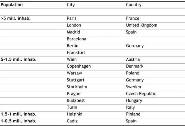
This paper is focused on a set of 16 cities from 12 countries. The Table 1 reveals those cities and respective countries, listed by category of number of inhabitants.

These cities were selected according to the data availability for the year 2015 and they will be studied according to three components: (i) Economic- where it is necessary to become efficient and competitive through dedicated investments to improve and maintain the infrastructure and the cost to users; (ii) Social - where there must be security, accessibility and equity in terms of access to transport; and (iii) Environmental - with concerns about energy consumption, the use of non-renewable sources, emissions and waste (see e.g. Alonso, et al., 2015; Haghshenas & Vaziri, 2012; Mahdinia, et al., 2018; Sustainable Transportation Indicators Subcommittee of the Transportation Research Board, 2008)

The data were mainly retrieved from a report of the European Metropolitan Transport Authorities (EMTA) where the associated are the responsible members for public transport in certain European cities. The remaining data come from several sources. The number of

Table 1: Cities under study

Population City Country

>5 mill. inhab. Paris France

London United Kingdom

Madrid Spain

Barcelona

Berlin Germany

Frankfurt

5-1.5 mill. inhab. Wien Austria

Copenhagen Denmark

Warsaw Poland

Stuttgart Germany

Stockholm Sweden

Prague Czech Republic

Budapest Hungary

Turin Italy

1.5-1 mill. inhab. Helsinki Finland

7

fatalities caused by accidents and the number of vehicles in circulation were collected from national statistics or from official reports from government organizations. The level of pollutants emissions was taken from the European Environment Agency and the price of gasoline in Statista statistics database.

For the indicators creation, there is certain requirements that should be considered. For instance, Litman (2008) argue that the indicators should be comprehensive and balanced relative to the areas that they are addressed representing sustainability. Furthermore, they should be valid, i.e. they should measure the feature that they are supposed. May et al. (2008) indicate that they must have easy understanding and sensitivity which means that they must become able to reveal changes. Lastly, the indicators must be standardized, available, measurable, reliable and unambiguous.

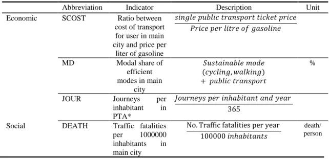
The literature was very helpful in order to understand which are the variables that are suitable for the formation of indicators. In previous studies, such as (Alonso, et al., 2015; Haghshenas & Vaziri, 2012; Haghshenas, et al., 2015), the environmental indicator was created by using the local emissions of pollutants in transport, public transport emissions, energy consumption in transport, area occupied by transport infrastructure. In economic level it is used local expenses dedicated to transport, transport costs, the average daily cost to the user, time spent in traffic. Last, for the social level it was resort the fatal road accidents, reduced public transport prices for students and senior citizens, accessibility in transport through the various systems available and the variety of transport. According to a previous literature review and with the appropriate transformations in the indicators formation it is possible to see in Table 2 how the indicators were constructed for this paper.

Table 2. Description of indicators

Abbreviation Indicator Description Unit

Economic SCOST Ratio between cost of transport for user in main city and price per

liter of gasoline 𝑠𝑖𝑛𝑔𝑙𝑒 𝑝𝑢𝑏𝑙𝑖𝑐 𝑡𝑟𝑎𝑛𝑠𝑝𝑜𝑟𝑡 𝑡𝑖𝑐𝑘𝑒𝑡 𝑝𝑟𝑖𝑐𝑒 𝑃𝑟𝑖𝑐𝑒 𝑝𝑒𝑟 𝑙𝑖𝑡𝑟𝑒 𝑜𝑓 𝑔𝑎𝑠𝑜𝑙𝑖𝑛𝑒 MD Modal share of efficient modes in main city 𝑆𝑢𝑠𝑡𝑎𝑖𝑛𝑎𝑏𝑙𝑒 𝑚𝑜𝑑𝑒 (𝑐𝑦𝑐𝑙𝑖𝑛𝑔, 𝑤𝑎𝑙𝑘𝑖𝑛𝑔) + 𝑝𝑢𝑏𝑙𝑖𝑐 𝑡𝑟𝑎𝑛𝑠𝑝𝑜𝑟𝑡 %

JOUR Journeys per inhabitant in PTA*

𝐽𝑜𝑢𝑟𝑛𝑒𝑦𝑠 𝑝𝑒𝑟 𝑖𝑛ℎ𝑎𝑏𝑖𝑡𝑎𝑛𝑡 𝑎𝑛𝑑 𝑦𝑒𝑎𝑟 365

Social DEATH Traffic fatalities per 1000000 inhabitants in main city

No. Traffic fatalities per year 100000 𝑖𝑛ℎ𝑎𝑏𝑖𝑡𝑎𝑛𝑡𝑠

death/ person

8

PT.NET Public transport network density in PTA* 𝐵𝑢𝑠 − 𝑟𝑎𝑖𝑙 𝑚𝑜𝑑𝑒𝑠 𝑙𝑒𝑛𝑔ℎ𝑡 𝑛𝑒𝑡𝑤𝑜𝑟𝑘 𝑘𝑚2 + 𝑚𝑒𝑡𝑟𝑜 − 𝑡𝑟𝑎𝑖𝑛 𝑙𝑒𝑛𝑔ℎ𝑡 𝑛𝑒𝑡𝑤𝑜𝑟𝑘 𝑘𝑚2 -

NUM.SS Public transport density in PTA* 𝑚𝑒𝑡𝑟𝑜&𝑡𝑟𝑎𝑖𝑛 𝑠𝑎𝑡𝑖𝑜𝑛𝑠 𝑘𝑚2 + 𝑏𝑢𝑠&𝑟𝑎𝑖𝑙 𝑚𝑜𝑑𝑒𝑠 𝑠𝑡𝑜𝑝𝑠 𝑘𝑚2 -

Environmental VEHC Inhabitants per vehicles in main city 𝐼𝑛ℎ𝑎𝑏𝑖𝑡𝑎𝑛𝑡𝑠 𝑁𝑜. 𝑜𝑓 𝑣𝑒ℎ𝑖𝑐𝑙𝑒𝑠 𝑖𝑛 𝑐𝑖𝑟𝑐𝑢𝑙𝑎𝑡𝑖𝑜𝑛 person/ vehicle PM Annual emissions of PM10 𝐴𝑛𝑛𝑢𝑎𝑙 𝑝𝑜𝑙𝑙𝑢𝑡𝑖𝑜𝑛𝑠 𝑜𝑓 𝑙𝑜𝑐𝑎𝑙 𝑎𝑖𝑟 𝑝𝑜𝑙𝑙𝑢𝑡𝑎𝑛𝑡 (𝑃𝑀10) µg/m3 URB % of urbanized surface in PTA* 𝑢𝑟𝑏𝑎𝑛𝑖𝑠𝑒𝑑 𝑠𝑢𝑟𝑓𝑎𝑐𝑒 𝑠𝑢𝑟𝑓𝑎𝑐𝑒 %

Notes: *PTA= Public Transport Authority

We have to note that variable urbanized surface of Copenhagen is used for the year 2013, because it was not available for 2015 and it should not have undergone major changes. In Cadiz, the ticket price was collected from an MMO report and the value of the urbanized surface is from 2012. PM10 pollutant values, for most of the cities are averages of urban local station measurements. The considered price of gasoline is associated to the national level gasoline prices.

9

4. Methodology

The composite indicators were used to create the sustainability indicator. Each composite indicator represents only one of the dimensions, i.e. economic, social and environmental. The formation of the composite indicators allows us to reflect complex or multidimensional realities, facilitating, through a comparative exercise, in solving issues in order to support decisions, being easy to interpret and separate indicators allowing thus, to include a set of information that would not be possible separately. Some examples of the methods for normalization process includes: categorical scales, percentage of differences, annual indicators above or below average over the consecutive year, re-scaling, classification, distance of a reference and standardization (Joumard et al., 2010). According with these authors the most used procedure is standardization. The standardization of the composite indicators will be performed such described in the eq. 1. Being this method sensitive to outliers, the cities that exhibit extreme values will be given greater weight (Alonso, et al., 2015).

The sub-indicators that integrate the composite indicators (eq. 2,3 and 4) could have a positive or negative signal as they are beneficial or not for efficient use of mobility (e.g. Alonso et al., 2015; Haghshenas & Vaziri 2012; Haghshenas et al., 2015). The lower prices for access to public transport encourage users to use it. Moreover, the enlargement of the infrastructures transport networks allows a better diversity of choice and improvements in mobility. A framework has been developed where it is possible to verify for each dimension what is intended to be more or less desirable to achieve the sustainability objectives (Litman, 2016).

To define the weights of the indicators it could be used different methods as referred by Danielis, et al. (2018). Therefore, the different options would be to give them: equal weighting; different weighting, attributed by specialists or general public ( e.g. De Andrade Guerra, et al., 2016); or group of correlated indicators describing the same sustainability dimension (PC/FA). To this study, as for Alonso, et al. (2015), Haghshenas & Vaziri (2012), Lopez-Carreiro & Monzon (2018) it was chosen to use equal weighting. IEC, ISOC, IAMB and ISUST correspond to economic,

social, environmental and sustainability indicators, respectively, and their results can be observed in table 6.

Formulation of composite indicators:

(1) 𝑍𝐼= 𝐼−𝐴𝑣𝑔𝐼 𝑆𝑡.𝐷𝑒𝑣𝐼 (2) IEC= −𝑆𝐶𝑂𝑆𝑇+ 𝑀𝐷 +𝐽𝑂𝑈𝑅 3

10

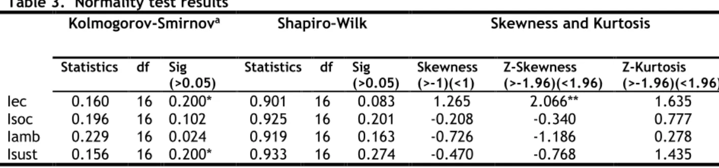
The Kolmogorov-Smirnov (K-S) and Shapiro-Wilk (S-W) tests were performed to validate the study by testing for the property of normality (Table 3). Please note that the use the Shapiro-Wilko test is appropriate for a sample ≤ 30 and advisable, for samples ≤ 50 while the Kolmogorov-Smirnov test is suitable in samples larger than 50 (Marôco, 2014).

The value of 0.024 in the environmental indicator and the value of 1.265 in the economic indicator are below the level of significance in relation to the K-S and Skewness test respectively. This can be explained due to the small sample. Sample size has immense importance in these tests. Minor observations, especially those below 30, may have a substantial impact on results, that is less advantageous. The greater the sample, the better its sensitivity and, consequently, more robust results (Yap & Sim, 2011; Hair et al., 2014).

According to Haghshenas & Vaziri (2012), Alonso et al (2015), and Lopez-Carreiro & Monzon, (2018) the Pearson's correlation was performed between certain city specifications, namely, GDP per capita, urban density, population and percentage of transport mobility type with the IEC, ISOC, IENV and ISUST (see Table 7).

Table 3. Normality test results

Kolmogorov-Smirnova _{Shapiro–Wilk Skewness and Kurtosis}

Statistics df Sig

(>0.05) Statistics df Sig (>0.05) Skewness (>-1)(<1) Z-Skewness (>-1.96)(<1.96) Z-Kurtosis (>-1.96)(<1.96) Iec 0.160 16 0.200* 0.901 16 0.083 1.265 2.066** 1.635 Isoc 0.196 16 0.102 0.925 16 0.201 -0.208 -0.340 0.777 Iamb 0.229 16 0.024 0.919 16 0.163 -0.726 -1.186 0.278 Isust 0.156 16 0.200* 0.933 16 0.274 -0.470 -0.768 1.435 Notes: *. This is a lower limit of true significance;

a. Correlation of Significance of Lilliefors

11

Then, to classify and group the cities according to their level of sustainability, the cluster analysis was carried out. In the hierarchical method, the starting number of the cluster is unknown. If it is to be discovered the non-hierarchical method were standing out by using a pre-established number. In a first step, the Ward method was used. It is more homogeneous in comparison to other methods, and the formation is made in order to both minimize the sum of the squares of the errors within the clusters and to maximize the sum of the squares of the errors between clusters (Marôco et al., 2014). In this method, the squared Euclidean distance was used because it is more adequate due to the existence of negative values (Alonso et al., 2015). As this procedure measures distances and may omit some dimension of sustainability due to the existence of different ranges in the indicators within the sample it was necessary to normalize again through z-scores, more fitting for this type of study (Hair et al., 2014).

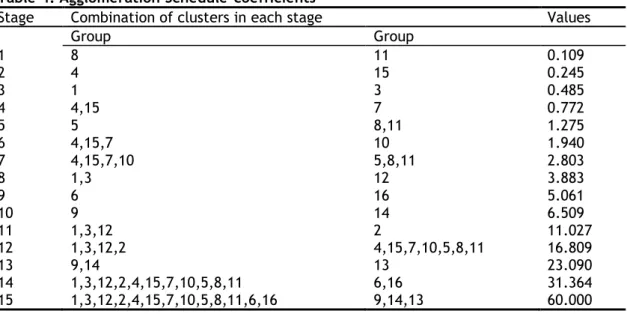
The determination of the appropriate number of clusters can be done through the analysis of a dendrogram (figure 1), or a graph (figure 2) obtained with the values of the coefficients of agglomeration schedule (table 4). Such as noted by Marôco (2014), these procedures are largely subjective. The R-Square-criteria were also used resorting to the one-way ANOVA. With the value of the coefficients relativized between 0 and 1 and with R-square, the graph was obtained (graph 1) where it is perceived that there is the formation of two clusters. In figure 3 and table 6 for cluster formation, there is a possibility of forming a further cluster in comparison to the previously used methods in which the formation of a cluster is composed of the greater part of the sample and does not separate the cities that shows an intermediate performance. Therefore, the formation of three clusters were chosen.

Table 4. Agglomeration Schedule-coefficients

Stage Combination of clusters in each stage Values

Group Group 1 8 11 0.109 2 4 15 0.245 3 1 3 0.485 4 4,15 7 0.772 5 5 8,11 1.275 6 4,15,7 10 1.940 7 4,15,7,10 5,8,11 2.803 8 1,3 12 3.883 9 6 16 5.061 10 9 14 6.509 11 1,3,12 2 11.027 12 1,3,12,2 4,15,7,10,5,8,11 16.809 13 9,14 13 23.090 14 1,3,12,2,4,15,7,10,5,8,11 6,16 31.364 15 1,3,12,2,4,15,7,10,5,8,11,6,16 9,14,13 60.000

12

Figure 1. Cluster arrangement

Figure 2. Number of cluster

To support the choice of the number of clusters, the k-means of the non-hierarchical method was used (Alonso et al., 2015). Thus, with k = 2 there were four iterations, and, in cluster

0 0,2 0,4 0,6 0,8 1 1,2 1 2 3 4 5 6 7 8 9 10 11 12 13 14 15 valu e no.clusters dist. R^2

13

allocation, there was no change. With k=3, only exists 3 interactions and there are some changes at the allocation level. It is possible to reorganize the cities in a different cluster comparing to the training done initially by the hierarchical method where the inclusion is definitive, reducing thus the probability of misclassification of a particular city and increasing the chances of putting it in the correct cluster (Marôco, 2014). However, if a reduced number of iterations and similarity exists between the final clusters, then it supports the stability of results (Hair, 2014).

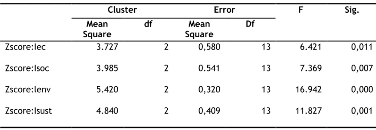
The results from the ANOVA analysis can be observed in Table 5. The F values show us the contribution of the variables to the classification of the cities, highlighting the environmental and sustainable indicators. In the cluster analysis, the p-value is irrelevant because it is desired that within the cluster, in this case, the cities are the most similar and outside the cluster as different as possible being the differences between clusters means significantly different in at least one of the variables. The objective is to highlight the variables that contribute to the formation of the clusters and are not different between them (Marôco, 2014).

In short, with the values obtained through the formation of the indicators, it was possible to classify the cities according to the various dimensions of sustainability. In a first phase, the optimum number of clusters had to be identified through the hierarchical method. In a second phase, with the k-means method the reliability of the result was tested. With the analysis ANOVA it was consolidated the formation of clusters.

Table 5. ANOVA analysis results from k-means procedure

Cluster Error F Sig.

Mean Square df Mean Square Df Zscore:Iec 3.727 2 0,580 13 6.421 0,011 Zscore:Isoc 3.985 2 0.541 13 7.369 0,007 Zscore:lenv 5.420 2 0,320 13 16.942 0,000 Zscore:Isust 4.840 2 0,409 13 11.827 0,001

14

5. Results and discussion

Through the level of sustainability, we can understand which cities have the best commitment to sustainable mobility, focusing more on public transport or non-motorized mobility methods. We can understand the concern about the transportation and welfare network through good infrastructure and quality of services because a certain part of the budget is used for investment.

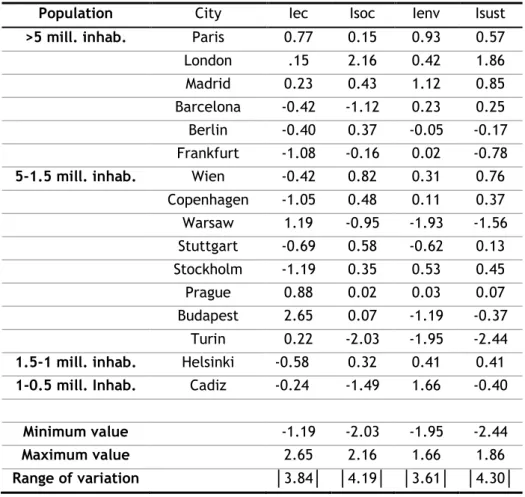
Table 6 shows the values of the indicators ordered by the city population. The negative values are less sustainable than the sample mean, while the positive values are more sustainable. At the economic, social and environmental level, the cities of Budapest, London and Cadiz stand out, respectively. London, Madrid and Paris stand out for the strengths performance with respect to the sustainability indicator and Turin, Warsaw and Frankfurt for weakness performance.

Table 6. Value of composite indicators for each city

Population City Iec Isoc Ienv Isust

>5 mill. inhab. Paris 0.77 0.15 0.93 0.57

London .15 2.16 0.42 1.86 Madrid 0.23 0.43 1.12 0.85 Barcelona -0.42 -1.12 0.23 0.25 Berlin -0.40 0.37 -0.05 -0.17 Frankfurt -1.08 -0.16 0.02 -0.78

5-1.5 mill. inhab. Wien -0.42 0.82 0.31 0.76

Copenhagen -1.05 0.48 0.11 0.37 Warsaw 1.19 -0.95 -1.93 -1.56 Stuttgart -0.69 0.58 -0.62 0.13 Stockholm -1.19 0.35 0.53 0.45 Prague 0.88 0.02 0.03 0.07 Budapest 2.65 0.07 -1.19 -0.37 Turin 0.22 -2.03 -1.95 -2.44

1.5-1 mill. inhab. Helsinki -0.58 0.32 0.41 0.41

1-0.5 mill. Inhab. Cadiz -0.24 -1.49 1.66 -0.40

Minimum value -1.19 -2.03 -1.95 -2.44

Maximum value 2.65 2.16 1.66 1.86

15

The results of the Pearson correlation are shown on Table 7. The correlation was performed between the indicators with certain characteristics of the cities. It should be noted that, the indicators were created following the data availability criteria. For these reasons some essential factors are partial or omitted such as revenues, expenditures and investments in relation to public transport. The GDP per capita of Helsinki corresponds to the year 2014 and in Cádiz this variable was collected from an OMM report. Instead of the relations obtained by Hashengan & Vaziri (2012), Alonso et al (2015) and Lopez-Carreiro & Monzon (2018), modes shares presents a positive correlation and the GDP per capita a negative correlation with the economic indicator. Urban density correlation is not significant across the social, environmental or sustainable indicators. As expected, the rest of motorized modes share have a negative correlation with the environmental indicator.

Table 7. Pearson correlation GDP per capita Urban density Sustainable modes share Public transport share Rest of motorized modes share Population in main city IEC Pearson correlation -0.519* 0.345 -0.377 0.662** -0.223 0.178 Sig. (2-tailed) 0.039 0.191 0.150 0.005 0.406 0.511 ISOC Pearson correlation 0.673** -0.374 -0.349 0.331 0.135 0.619* Sig. (2-tailed) 0.004 0.153 0.185 0.221 0.617 0.011 IENV Pearson correlation 0.361 0.066 0.528* -0.307 -0.503* 0.126 Sig. (2-tailed) 0.169 0.808 0.036 0.247 0.047 0.642 ISUST Pearson correlation 0.659** -0.243 -0.046 0.145 -0.135 0.542* Sig. (2-tailed) 0.005 0.365 0.866 0.593 0.619 0.030

Notes: *, **. Correlation is significant at the 0.05 and 0.01 levels (2-tailed), respectively.

With higher GDP per capita, it is assumed that there is more investment regarding to public transport and its infrastructures, allowing a better quality of the network. This increase in quality of service presents an increase in prices for users and the increase of costs for public authorities. These evidences may explain the negative relationship with the economic indicator. On the other hand, the positive relationship of this indicator with the percentage of public transport indicates that the increase in public transport and its diversity increase the demand for these goods and the number of trips.

16

The negative relationship between GDP per capita and the social indicator could mean that economic growth has not improved the social development of transport, which could indicate, that there is little investment in social welfare. However, concerned cities that are aware of environmental impacts have higher GDP per capita, reflecting the economic and social level allowing a positive correlation with the sustainability indicator.

More populated cities are usually denser because the number of people is much higher, but the city’s area does not increase proportionally when compared to less populous cities. In these more populous European cities, usually, there is more concern about mobility, pollution and well-being. There may be more support and investments to sustainable transportation and infrastructure. This could explain the positive relationship between the population and both the social and sustainability indicators.

The percentage of motor vehicles are negatively correlated with environmental indicators while the percentage of sustainable models are positively correlated with it. These findings could show the importance that is given to non-motorized modes. This mean that cities with larger urban areas tend to have more vehicles in circulation due to the increased travel time spent making it difficult to use other mobility methods. Some policies have been designed to reduce the use of private vehicles in green zones where vehicles are only allowed to circulate if they meet certain emission requirements. Additionally, there are areas where the use of vehicles is prohibited except for residents.

In figure 3 and table 8, it is shown the characteristics and profile of the clusters formed. Figure 3 shows a three-dimensional chart with the environmental, economic and social indicator. It is visible the formation and distinction of the cluster formed with the cities of Turin, Warsaw and Budapest due to a poor environmental performance compared to other cities.

17

Figure 3. Clusters with economic, social and environmental indicators scores.

Cluster 1 consists of five cities, namely Paris, Frankfurt, Barcelona, Prague and Cádiz, cluster 2 with eight, London, Madrid, Berlin Wien, Copenhagen, Stuttgart, Stockholm and Helsinki and the cluster 3 with three, Warsaw, Budapest and Turin. In terms of indicators, except at the economic level, the cluster 3 shows a weakness in the remaining indicators. Cluster 2 stands out to social and sustainable indicators and cluster 1 at the environmental level.

Table 8. Average profiles of cities in each cluster (centroid values) Clusters (k-means method)

1 Environmentally efficient 2 Social friendly 3 Economic competitive IEC -0.01 -0.50 1.35 ISOC -0.52 0.69 -0.97 IENV 0.57 0.28 -1.69 ISUST -0.14 0.63 -1.46

Sustainable modes share (%) 0.47 0.35 0.26

Public transport share (%) 0.27 0.31 0.40

Rest of motorized modes

chare 0.25 0.33 0.34

GDP per capita (Є) 32652.60 46008.13 19990.67

Urban density (inhab. /𝒌𝒎𝟐₎

5254.27 3451.64 6065.67

Population in main city

18

In the economic indicator, cluster 2 performance is below average. It may be due to the practice of higher ticket prices. The ratio of a single ticket price with the price per liter of gasoline is about 1.9 which may indicate a high level of welfare. In comparison, cluster 3 presents a ratio of 0.96 which could show that the ticket price is lower contributing to the use of public transport, and a high value of total daily journeys per inhabitant.

In the environmental indicator, cluster 3 presents a relatively higher PM10 emissions (≈39 µg/m3) and for each vehicle there are two people in contrast with cluster 2 that have 9 people for each vehicle. This tells one that as the ratio of inhabitants per vehicle increases it shows a reduction in the use of private motorized vehicles and consequently lower emissions.

In the social indicator, cluster 3 presents the highest number of deaths per million inhabitants with approximately 41 deaths where cluster 2 presents only 13. Interestingly, cluster 3 presents a higher percentage of public transport use, but in contrast a low percentage at the level of sustainable modes in comparison to cluster 1. Cities with greater population concentration are more likely to receive support for a better investment. Cluster 3 shows a greater urban density but at the level of GDP per capita, it is much lower, which could indicate that there is less investment than in the other clusters, as well as income allocated to improve the urban mobility.

5.1 Robustness

To compare cities evolution, the same methodology was applied for data from the year 2012. Please note that these results cannot be directly compared with the analysis performed for the year 2015. This is because the group of cities present in the sample is not exactly the same as the one presented in the main analysis. Of the 16 cities used in each analysis, only 12 are common. Thus, the 12 common cities common to both analysis are: Budapest, Paris, Turin, Barcelona, Helsinki, Madrid, Berlin, Copenhagen, London, Prague, Stockholm and Warsaw. The remaining four cities used in the year 2012 are: Brussels, Montreal, Oslo and Hamburg. In 2015 the four cities used are: Cadiz, Frankfurt, Vienna and Stuttgart. Although the sample of cities is not completely equal for the two analyzed years and therefore not being possible to make a direct analysis, one can still in a way contrast the two analyses. This is the reason why this subsection could be seen as a kind of robustness analysis, due to the limitations of the analysis upon only 16 observations.

In the formation of the indicators some of the variables used are different due to the different availability of data in 2012 and in 2015. In table 9, it is possible to see the construction of the indicators for 2012 and underlined the variables that are different from the main study. This table also indicates the signal given to the variables for the construction of the indicators as well as the source from which they were withdrawn.

19

Table 9. Formation of indicators for the year 2012

Indicator Unit Desired

sign

Source Economic Coverage of operational

costs by fare revenues

% - EMTA

Single ticket fare in main city (€) /gasoline liter price (unleaded 95

in 2011, €)

- EMTA

Total journeys per inhabitant and day

+ EMTA

Social Traffic fatalities per

thousand inhabitants Death/person - Nacional/Regional statistics or official report Public transport modes

operate -

+ UITP

Total public transport vehicle kilometers per

inhabitant

Km/inhabitant + UITP

Environmental Passenger cars per

inhabitants inhabitant Vehicles/ - UITP Estimated average

exposure to air pollution (PM2.5) Micrograms per cubic metre - OECD Proportion of the metropolitan area's surface which is urbanized % - UITP

Note: the variable estimated average exposure to air pollution (PM2.5) It is referent for the year 2013

About normality, Table 10 shows that all the indicators have a normal distribution. In the formation of the clusters, the existence of three groups without ambiguity is observable. The first group consists of: Brussels, Budapest, Hamburg, Paris and Turin. The second group consists of: Barcelona, Helsinki, Madrid, Montreal and Oslo. The third group by: Berlin, Copenhagen, London, Prague, Stockholm and Warsaw.

Table 10. Tests of Normality for the year 2012

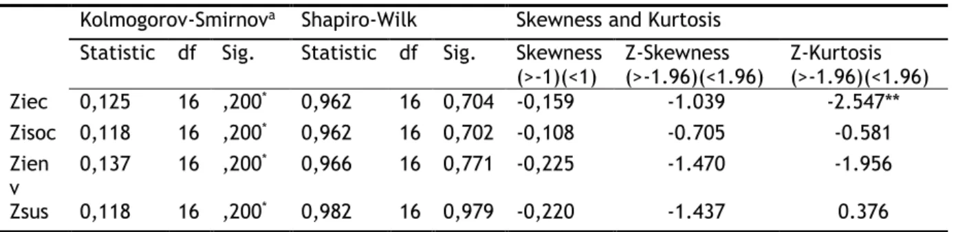
Kolmogorov-Smirnova _{Shapiro-Wilk Skewness and Kurtosis}

Statistic df Sig. Statistic df Sig. Skewness (>-1)(<1) Z-Skewness (>-1.96)(<1.96) Z-Kurtosis (>-1.96)(<1.96) Ziec 0,125 16 ,200* _{0,962 16 0,704 -0,159 -1.039 -2.547**} Zisoc 0,118 16 ,200* _{0,962 16 0,702 -0,108 -0.705 -0.581} Zien v 0,137 16 ,200 * _{0,966 16 0,771 -0,225 -1.470 -1.956} Zsus 0,118 16 ,200* _{0,982 16 0,979 -0,220 -1.437 0.376}

*. This is a lower bound of the true significance. a. Lilliefors Significance Correction

20

Since the cities of the two analyses are not completely equal, it is possible that cities that are in a cluster in the year 2015 be in another one in the year 2012. This is due, besides the evolution of the cities, the possible reorganization of clusters due to cities who are not in the 2012 sample to be stronger or weaker than the cities present in the other year and vice versa. In table 11 one can see the results for the cluster for the year 2012.

Table 11. Average profiles of cities in each cluster (centroid values) for the year 2012

Clusters (k-means method)

1 2 3

IEC 0.49 -0.71 0.18

ISOC -0.70 -0.53 1.03

IENV -0.84 1.01 -0.14

ISUST -0.79 -0.39 0.99

Sustainable modes share (%) 0.39 0.36 0.32

Public transport share (%) 0.27 0.32 0.37

Rest of motorized modes chare 0.34 0.33 0.30

GDP per capita (Є) 32300 42325 39133

Urban density (inhab./𝒌𝒎𝟐₎

1390.6 872.6 1218.67

Population (inhabitants) 2530000 3496000 4882333

In the economic indicator, cluster 1, although it is not the one with the largest number of total journeys per inhabitant per day, is the one that presents the best performance since the cities that comprise it are those that present a lower ratio between the price of the ticket and the price of gasoline per liter and on average less than 1. This is a characteristic that contributes to the use of public transport. On the other hand, in Cluster 3, with the highest ratio between the price of the ticket and the gasoline price per liter (≈1.43), it has the highest number of total journeys per inhabitant per day.

In the social indicator, cluster 3 is the one with the best performance. This indicator is strongly influenced by the total public transport vehicle km per inhabitant which suggests that there may be a denser public transport network. This was already foreseen since the ratio between the price of the ticket and the price of gasoline per liter is the highest, indicating a possible stronger share of welfare.

In the environmental indicator, cluster 2, with lower urban density, is the one that performs better. This is due in large part to the "estimated average exposure to air pollution (PM2.5)" in which the presence of this particle, in micrograms per cubic meter, is lower.

Despite the differences in both cities and variables mentioned above, it is still possible to draw some conclusions. In these conclusions the values of the indicators cannot be compared since

21

the process of formation of the indicators differs. However, it is possible to perceive that clusters or cities are stronger in these indicators even with different formations. For example, for the year 2015 cluster 2 is the one that shows the best performance in the global indicators. The same can be observed in cluster 3 of the data for 2012. This happens because the various cities that make up these two clusters coincide, for example: London, Berlin, Copenhagen and Stockholm. In these two analyzes it is possible to observe the importance of the social indicator, since it shows us the development of the public transport service.

22

6. Conclusions

Cities have dealt with problems derived from the increased concentration of population density, creating serious problems in terms of accessibility, mobility and pollution. Generators of a good share of wealth need to become more and more intelligent where the transport sectors play a key role in dealing with these challenges.

Understanding how cities have progressed over the years to the level of sustainability and environmental problems combined with the policies already implemented, would be a useful tool to help the policymakers on how to proceed towards more sustainable and efficient cities. With the available data, it was possible to create economic, social, environmental and sustainability indicators. This paper studied 16 European cities for the year 2015, with the aim of having the reality of the differences between countries for a better understanding of the sustainability across Europe. A Pearson’s correlation was performed between the 4 indicators and city’s specifications. With these indicators a cluster analysis was performed.

Some characteristics of cities stand out in sustainability, such as small and denser cities that have a good performance. Also, richer cities tend to have a more sustainable performance. Cities with a higher percentage of urbanization have difficulties in having sustainable modes so optimized.

In accordance with the cluster disposition, it has been realized that most of the cities under study promote the use of public transport and give more and more importance to the type of non-motorized mobility. This may be due to the fact that the cities under study are European and have invested in improving infrastructures and networks, for example, by creating specific mobility policies.

With the aim of understanding the evolution of cities, a second analysis was carried out for 2012. In this analysis, which cannot be directly compared, due to differences in the formation of indicators and in the composition of the sample of cities, it is noticed that in some ways the same cities tend to be in clusters with the same trend as the main model.

For future research, the performance observed can be compared with other years. In this sense, future research should enlarge the sample analyzed, considering other cities to improve the model. Additionally, the projects or restrictive policies focused on mobility access, pollution should be analyzed to check their impact on the stated objectives. Notwithstanding, the inclusion of the other areas, such as technological innovation and progress could greatly contribute to improve the knowledge on the smart cities and sustainability.

23

7. References

Alonso, A., Monzón, A., & Cascajo, R. (2015). Comparative analysis of passenger transport sustainability in European cities. Ecological Indicators, 48, 578–592. https://doi.org/10.1016/j.ecolind.2014.09.022

Bibri, S. E., & Krogstie, J. (2017). Smart sustainable cities of the future: An extensive interdisciplinary literature review. Sustainable Cities and Society, 31, 183–212. https://doi.org/10.1016/j.scs.2017.02.016

Corazza, M. V., Guida, U., Musso, A., & Tozzi, M. (2016). A new generation of buses to support more sustainable urban transport policies: A path towards “greener” awareness among bus stakeholders in Europe. Research in Transportation Economics, 55, 20–29. https://doi.org/10.1016/j.retrec.2016.04.007

Danielis, R., Rotaris, L., & Monte, A. (2018). Composite indicators of sustainable urban mobility: Estimating the rankings frequency distribution combining multiple methodologies.

International Journal of Sustainable Transportation, 12(5), 380-395.

De Andrade, J. B. S. O., Ribeiro, J. M. P., Fernandez, F., Bailey, C., Barbosa, S. B., & da Silva Neiva, S. (2016). The adoption of strategies for sustainable cities: A comparative study between Newcastle and Florianópolis focused on urban mobility. Journal of Cleaner Production, 113, 681-694.

Eurostat. (2017). Greenhouse gas emission statistics - emission inventories, 2015(June 2017), 1–7. Retrieved from http://ec.europa.eu/eurostat/statistics-explained/index.php/Greenhouse_gas_emission_statistics_-_emission_inventories

Glotz-Richter, M., & Koch, H. (2016). Electrification of Public Transport in Cities (Horizon 2020 ELIPTIC Project). Transportation Research Procedia, 14, 2614–2619. https://doi.org/10.1016/j.trpro.2016.05.416

Hair, J. F., Black, W. C., Babin, B. J., & Anderson, R. E. (2014). Multivariate data analysis (Vol. 5, No. 3, pp. 207-219). Upper Saddle River, NJ: Prentice hall.

Haghshenas, H., & Vaziri, M. (2012). Urban sustainable transportation indicators for global

comparison. Ecological Indicators, 15(1), 115–121.

24

Haghshenas, H., Vaziri, M., & Gholamialam, A. (2015). Evaluation of sustainable policy in urban transportation using system dynamics and world cities data: A case study in Isfahan. Cities, 45, 104–115. https://doi.org/10.1016/j.cities.2014.11.003

Joumard, R., Gudmundsson, H., Arapis, G., Arce, R., & Aschemann, R. (2010). Indicators of

environmental sustainability in transport. An interdisciplinary approach to methods.

Karkatsoulis, P., Siskos, P., Paroussos, L., & Capros, P. (2017). Simulating deep CO2 emission reduction in transport in a general equilibrium framework: The GEM-E3T model. Transportation

Research Part D, 55, 343–358. https://doi.org/10.1016/j.trd.2016.11.026

Klinger, T., Kenworthy, J. R., & Lanzendorf, M. (2013). Dimensions of urban mobility cultures - a comparison of German cities. Journal of Transport Geography, 31, 18–29. https://doi.org/10.1016/j.jtrangeo.2013.05.002

Lopez-Carreiro, I., & Monzon, A. (2018). Evaluating sustainability and innovation of mobility patterns in Spanish cities. Analysis by size and urban typology. Sustainable Cities and Society,

38(February), 684–696. https://doi.org/10.1016/j.scs.2018.01.029

Macedo, J., Rodrigues, F., & Tavares, F. (2017). Urban sustainability mobility assessment:

Indicators proposal.Energy Procedia, 134, 731–740.

https://doi.org/10.1016/j.egypro.2017.09.569

Marôco, J. (2014). Análise estatística com o SPSS Statistics 6th edn Lisboa:. ReportNumber, Lda.

Mahdinia, I., Habibian, M., Hatamzadeh, Y., & Gudmundsson, H. (2018). An indicator-based algorithm to measure transportation sustainability: A case study of the U.S. states. Ecological

Indicators, 89(March 2017), 738–754. https://doi.org/10.1016/j.ecolind.2017.12.019

Maria, J., Lopez-lambas, M. E., Gonzalo, H., Rojo, M., & Garcia-martinez, A. (2018). Methodology for assessing the cost effectiveness of Sustainable Urban Mobility Plans (SUMPs). The case of the city of Burgos. Journal of Transport Geography, 68(January), 22–30. https://doi.org/10.1016/j.jtrangeo.2018.02.006

May, A. D., Page, M., & Hull, A. (2008). Developing a set of decision-support tools for sustainable urban transport in the UK. Transport Policy, 15(6), 328–340.

https://doi.org/10.1016/j.tranpol.2008.12.010

Naganathan, H., & Chong, W. K. (2017). Evaluation of state sustainable transportation performances (SSTP) using sustainable indicators. Sustainable cities and society, 35, 799-815.

25

Rotmans, J., Van Asselt, M., & Vellinga, P. (2000). An integrated planning tool for sustainable cities. Environmental Impact Assessment Review, 20(3), 265–276. https://doi.org/10.1016/S0195-9255(00)00039-1

Sustainable Transportation Indicators Subcommittee of the Transportation Research Board. (2008). Sustainable Transportation Indicators. Transportation, 65(November), 1–20. Retrieved from http://www.centreforsustainabletransportation.org/researchandstudies.htm

Tamaki, T., Nakamura, H., Fujii, H., & Managi, S. (2016). Efficiency and emissions from urban transport: Application to world city-level public transportation. Economic Analysis and Policy, (1992). https://doi.org/10.1016/j.eap.2016.09.001

Litman, T. 2016. "Well Measured", 10–15.

United Nations, Department of Economic and Social Affairs, P. D. 2014. "World Urbanization Prospects". United Nations, 32.Yap, B. W., & Sim, C. H. (2011). Comparisons of various types of normality tests. Journal of Statistical Computation and Simulation, 81(12), 2141-2155. CIVITAS - cleaner and better transport in cities

http://civitas.eu/about-us-page

European Comission – Mobility and Transport

https://ec.europa.eu/transport/themes/strategies/news/2016-07-20-decarbonisation_en https://ec.europa.eu/transport/themes/logistics-and-multimodal-transport/multimodal-and-combined-transport_en