Study of the Thermal Behavior of a Three-phase Induction Motor under Fault Conditions

(1)

UNIVERSIDADE DA BEIRA INTERIOR

Engineering

Study of the Thermal Behavior of a Three-phase

Induction Motor under Fault Conditions

Fábio Emanuel Pereira Santiago

Dissertation for obtaining the degree of Master of Science in

Electrical and Computer Engineering

(2

nd

_{cycle of studies)}

Advisor: Prof. Dr. António João Marques Cardoso

Co-advisor (external): Prof. Dr. Konstantinos N. Gyftakis

Co-advisor: Prof. Dr. João Manuel Milheiro Caldas Paiva Monteiro

(2)

(3)

Acknowledgments

I would like to start by acknowledging all my family, especially my parents and sister, for the support given during this long journey.

I would also like to say that I am grateful to my MSc Dissertation advisor, Prof. Dr. António João Marques Cardoso, for the suggested theme and supervision, as well as the opportunity for working at CISE - Electromechatronic Systems Research Centre, where I was able to work with some laboratory equipment, in order to accomplish this work.

I would also like to thank my external co-advisor, Prof. Dr. Konstantinos N. Gyftakis, for the priceless help and all the support provided throughout this year.

Without forgetting all my co-workers and friends, I would like to thank them for the advices and companionship, in particular to Saúl Sales, Fernando Bento and Carlos Santos.

Finally, a very special word to my girlfriend Ana Nunes.

It was an honor being able to have all these people at my side. Without them I would not be able to accomplish this work.

(4)

(5)

Resumo

Os motores elétricos desempenham um papel bastante importante na indústria, pois hoje em dia quase tudo na indústria funciona com o auxílio destes, seja em reduzidas ou elevadas potências. É possível dividir os motores elétricos em motores de indução e motores síncronos, no entanto os mais utilizados na indústria são os de indução, sendo então bastante importante monitorizar o seu comportamento ao longo do tempo. Devido às suas condições de funcionamento, que por vezes são bastante adversas, as perdas do motor podem aumentar causando a degradação dos materiais e levando a falhas graves, que podem prejudicar toda a produção de uma indústria, infligindo graves perdas financeiras

O objetivo principal desta dissertação é criar um modelo computacional de um motor de indução trifásico de rotor em gaiola de esquilo para estudar e analisar o seu comportamento térmico, tanto sob condições normais como de avaria. Este trabalho será desenvolvido através do método de elementos finitos (FEM), sendo assim utilizado o software Flux2D 12.1 (Cedrat). Inicialmente a modelação computacional focar-se-á no estudo eletromagnético, de forma a calcularem-se as perdas do motor. Posteriormente, esses valores serão inseridos na simulação térmica, de forma a compreender-se melhor o comportamento térmico do motor.

Os ensaios experimentais terão o auxílio de cinco sensores de temperatura (PT100) onde a aquisição dos dados experimentais é efetuada através de um software desenvolvido na linguagem de programação LabView. Posteriormente, os resultados obtidos experimentalmente serão comparados com os resultados obtidos computacionalmente. Porém, apenas os resultados de dois dos sensores podem ser comparados, pois existem dois sensores ao longo da perspetiva tridimensional do motor e um que está situado na periferia interna da carcaça, a qual não será definida na simulação.

Palavras-chave

Comportamento térmico; Perdas energéticas; Motor de indução de rotor em gaiola de esquilo; Métodos de Elementos Finitos; Condição de avaria.

(6)

(7)

Abstract

Electric motors play an important role in the industry, because nowadays almost everything in the industry works with the auxiliary of them, either for low or high power ratings. It is possible to divide the electric motors in induction motors and synchronous motors, however the most used in the industry are the induction motors. So, it is very important to monitor its behavior throughout the time. Due to their working conditions, which sometimes can be very adverse, the motor losses can increase the inner machine temperature causing degradation of the materials which will lead to serious faults. Most severe faults may lead to a machine breakdown and interruption of the industrial production inflicting severe financial loss.

The main goal of this dissertation is to create a computational model of a three-phase squirrel cage induction motor to study and analyze its thermal behavior under healthy and faulty conditions. This will be made through the finite elements method (FEM), where Flux2D 12.1 (Cedrat) software will be used. Initially the computational modeling will focus on the electromagnetic study, in order to calculate the motor losses. After that, those values will be inserted in the thermal simulation to better understand the thermal behavior of the motor.

The experimental tests will be carried out with the aid of five temperature sensors (PT100), where the acquisition of the experimental data will be done through a software developed in LabView programming language. As well as that, the results obtained experimentally will be compared with those obtained computationally. However, only the results of two sensors can be compared, since two of them are placed throughout the three-dimensional perspective of the motor and one is placed inner of the motor frame, which will not be defined in the simulation.

Keywords:

Thermal behavior; Power losses; Three-phase squirrel cage induction motor; Finite Elements Method; Fault condition.

(8)

(9)

Index

1. Introduction ... 1 1.1. Background ... 1 1.2. Motivation ... 4 1.3. Objectives ... 5 1.4. State of Art ... 5 1.4.1. Induction Machine ... 5 1.4.2. Constructive Features ... 6 1.4.3. Methods ... 7

1.5. Overview and Organization of the Dissertation ... 8

2. Steady State Condition ... 9

2.1. Constructive Features ... 9

2.2. Electromagnetic Modeling and Simulation ... 11

2.2.1. Geometry ... 11

2.2.2. Assign Regions to Faces ... 12

2.2.3. Mesh Creation ... 14 2.2.4. Materials Definition ... 15 2.2.5. Mechanical Sets ... 16 2.2.6. Boundary Regions ... 17 2.2.7. Electric Circuit ... 17 2.2.8. Solving Scenario... 19 2.2.9. Results Analysis ... 20 2.2.10. Losses Calculation ... 22 2.3. Thermal Simulation ... 25

2.3.1. Thermal Simulation Results ... 27

3. Transient State Condition ... 35

3.1. Electromagnetic Simulation ... 35

3.1.1. Mechanical Sets ... 35

(10)

3.1.3. Solving Scenario ... 37

3.1.4. Results Analysis ... 37

3.1.5. Losses Calculation ... 41

3.2. Analysis of Thermal Simulation Results ... 42

4. Supply Voltage Unbalances ... 45

4.1. Amplitude Unbalance in Supply Voltages ... 45

4.1.1. Electromagnetic Simulations ... 48

4.1.3. Electromagnetic Experimental Tests ... 50

4.2. Phase Unbalance in Supply Voltages ... 51

4.3. Mixed Unbalance in Supply Voltages ... 54

4.4. Comparison between Simulation and Experimental Tests ... 57

4.4.1. Thermal Results... 57

4.4.2. Thermal Images ... 59

5. Conclusions and Suggestions for Future Works ... 63

5.1. Conclusions ... 63

5.2. Suggestions for Future Works... 64

(11)

List of Figures

Fig. 1.1 – Losses diagram of an induction motor. ... 3

Fig. 2.1 – Winding scheme (WEG courtesy). ... 10

Fig. 2.2 – Motor geometry. ... 11

Fig. 2.3 – Assignment of regions to faces (Flux2D). ... 12

Fig. 2.4 – Faces of phase U (Flux2D). ... 13

Fig. 2.5 – Faces of phase V (Flux2D). ... 13

Fig. 2.6 – Faces of phase W (Flux2D). ... 13

Fig. 2.7 – Motor mesh (Flux2D). ... 14

Fig. 2.8 – Boundary lines – Electromagnetic simulation (Flux2D). ... 17

Fig. 2.9 – Electric circuit scheme (Flux2D). ... 18

Fig. 2.10 – Input currents as a function of the slip (Flux2D). ... 20

Fig. 2.11 – Torque as a function of the slip (Flux2D). ... 21

Fig. 2.12 – Mechanical power as a function of the slip (Flux2D). ... 22

Fig. 2.13 – Power loss curve characteristic of silicon steel as function of the peak flux density (WEG courtesy). ... 24

Fig. 2.14 – Boundary lines – Thermal simulation (Flux2D). ... 27

Fig. 2.15 – Motor thermal behavior at the time: a) 0s; b) 300s; c) 600s; d) 1000s; e) 2000s; f) 3000s; g) 4000s; h) 5000s; i) 6000; j) 10000s ... 28

Fig. 2.16 – Motor thermal behavior after 600s (Flux2D). ... 29

Fig. 2.20 – Motor thermal behavior after 10000s (Flux2D)... 33

Fig. 3.1 – Introduced torque (Flux2D). ... 36

Fig. 3.2 – Supply voltages along 0.5 seconds (Flux2D)... 37

Fig. 3.3 – Close view of the Fig. 3.2 (Flux2D). ... 38

Fig. 3.4 – Supply currents along 0.5 seconds (Flux2D). ... 38

Fig. 3.5 – Speed along 0.5 seconds (Flux2D). ... 39

Fig. 3.6 – Torque load along 0.5 seconds (Flux2D). ... 40

Fig. 3.7 – Mechanical power along 0.5 seconds (Flux2D). ... 40

Fig. 3.8 – Sensors placement in two-dimensional model. ... 42

Fig. 3.9 – Comparison between simulation and experimental thermal results. ... 43

Fig. 4.1 – Power factor as a function of different voltage unbalance levels [41]. ... 47

Fig. 4.2 – Phasor diagram of a symmetrical three-phase voltage supply system. ... 51

Fig. 4.3 – Comparison between PVU and VUF along the V phase angle. ... 52

Fig. 4.4 – Trend curve of the total amount of losses as a function of the phase displacement. ... 53

(12)

Fig. 4.5 – Comparison between the trend curves of the final motor’s temperatures along the total phase displacement. ... 58 Fig. 4.6 – Experimental thermal images of the double amplitude unbalance case, captured with a thermal camera. ... 59 Fig. 4.7 – Simulation thermal image of the double amplitude unbalance case (Flux2D). ... 60 Fig. 4.8 – Experimental thermal images of the phase unbalance case with the highest phase displacement in one single phase, captured with a thermal camera. ... 61 Fig. 4.9 – Simulation thermal images of the phase unbalance case with the highest phase displacement in one single phase (Flux2D). ... 61

(13)

List of Tables

Table 1.1 – Type and percentage distribution of the total losses in an induction motor [30]. .. 4

Table 2.1 – Association of the material to its respective face. ... 16

Table 2.2 – Mechanical set of each face. ... 16

Table 2.3 – Values of the electric circuit components. ... 19

Table 2.4 – Assignment of the components to the coils. ... 19

Table 2.5 – Assignment of the components to the bars. ... 19

Table 2.6 – Solving scenario – steady state. ... 20

Table 2.7 – Stator and rotor iron losses. ... 24

Table 2.8 – Faces configuration for thermal simulation. ... 26

Table 3.1 – Supply voltages of the electric circuit – transient state. ... 36

Table 3.2 – Solving scenario – transient state. ... 37

Table 3.3 – Iron losses at rated-load condition. ... 42

Table 3.4 – Simulation and experimental thermal values after 10000 seconds. ... 43

Table 4.1 – Input simulation data for amplitude unbalances. ... 48

Table 4.2 – Simulation results of the Joule and iron losses for amplitude unbalances. ... 49

Table 4.3 – Input experimental data for amplitude unbalances. ... 50

Table 4.4 – Input simulation data for phase unbalances at half-load condition. ... 52

Table 4.5 – Simulation results of the Joule and iron losses for phase unbalances at half-load condition. ... 53

Table 4.6 – Input experimental data for phase unbalances at half-load condition. ... 54

Table 4.7 – Input simulation data for mixed unbalances at half-load condition. ... 55

Table 4.8 – Simulation results of the Joule and iron losses for mixed unbalances at half-load condition. ... 56

Table 4.9 – Input experimental data for mixed unbalances at half-load condition. ... 56

Table 4.10 – Comparison between experimental and simulation thermal results for all the different cases. ... 57

(14)

(15)

List of Acronyms

AC Alternating Current

CFD Computational Fluid Dynamics FEM Finite Elements Method

IEC International Electrotechnical Commission LPTN Lumped Parameters Thermal Network

LS Loss Surface

NEMA National Equipment Manufacturers Association PVU Percentage of Voltage Unbalance

RMS Root Mean Square

(16)

(17)

Chapter 1

Introduction

1.1. Background

The induction machine, also known as the asynchronous machine, can operate both as motor or generator. Most of the times it is used as motor, because its performance features as generator are unsatisfactory for most applications. There is no specific size or power for these motors, so there is a wide range of choice, since small single-phase induction motors for use in various domestic applications, until large three-phase induction motors of high power ratings, used in an industrial level. There are also linear induction motors, mostly used in transportation systems. Induction motors are widely used in industry, being the key elements that ensure the continuity of the development process and the production chain [1].

Three-phase induction motors have high industrial reputation, because they have very advantageous features, such as, their robustness, simplicity, reliability, excellent adaptation to different loads and different working conditions, low operating cost and low maintenance level [1]-[5].

As these motors sometimes need to operate in extreme industrial environments, they also require periodic maintenance in order to avoid possible breakdowns that can interrupt the entire production process. Since overheating is one of the most severe root causes of certain faults, it is important to study the thermal behavior of the induction motor to prevent catastrophic events, to reduce repair cost and to extend the motor life time.

The temperature increase in electric motors is a subject that has been arousing more and more interest due to being an important factor for the motor operational performance, since this can affect its operational safety. Information about faults in electric motors can be retrieved throughout literature [6], pointing out unbalanced voltage supplies [7]-[8], short-circuits on the stator winding [9]-[11], broken rotor bars [12]-[18] and eccentricity [17]-[25].

Through the Arrhenius equation, it is possible to state that the chemical reaction speed varies with temperature. Montsinger adapted this equation to establish a rule that relates the insulation behavior to the operating temperature of the machine, entitled “Rule 10”. According to this rule, for each 10 ºC increase (above the temperature under rated conditions) in the

(18)

windings insulation temperature, there will be about 50 % decrease in the insulation life time [25]-[27].

The way the motor works is a very important factor for good motor preservation, however this is not the only one. The external motor conditions, or in other words, the surrounding environment of the motor is crucial for its proper operation, so it is necessary to respect two important conditions - the environment temperature and the operation altitude, due to air rarefaction. The motor in question behaves normally up to 1000 meters above the sea level and at temperatures between -20 ºC and +40 ºC. If these conditions were not respected, the motor will not be able to provide its rated power and the losses may increase, making it more difficult to dissipate heat, which could damage some parts of the motor, particularly the windings’ insulation [28].

The losses in the induction motor are divided into four groups: electrical, magnetic, mechanical and parasitic losses. Electrical losses, also called Joule losses, vary with the current and with the resistance of both stator windings and rotor bars. It is possible to reduce those losses by increasing the cross section of stator and rotor conductors. Magnetic losses can be called core losses or iron losses. These include hysteresis and eddy current losses, which can be reduced by the use of high quality silicon steel and by decreasing the rolling area of the magnetic plates in the core, respectively. The core losses depend on the flux density and on the frequency of the supply voltage (f1). The frequency is much lower in the rotor core, assuming values about 3%, compared to the stator supply frequency (f1), since the frequency value induced in the rotor (f2) is equal to the product of the stator supply voltage frequency (f1) and the slip (f2 = sf1). For example, for a f1 equals to 50 Hz, there will be a f2 of about 1.5 Hz. Mechanical losses, also called friction and ventilation losses, are influenced by ventilation and friction in the bearings. These losses increase proportionally with the increase of the speed. In order to reduce these losses, it is necessary to use low friction bearings and to improve the ventilation system. The parasitic losses are the result of leakage of flow, non-uniform current distribution and mechanical imperfections. It is necessary to be very careful in the optimization of the design and in the manufacture of the motor, so that this kind of losses can be reduced [29]. Fig. 1.1 shows the Sankey diagram of the power flow and losses of an induction motor.

(19)

Study of the Thermal Behavior of a Three-phase Induction Motor Under Fault Conditions

Fig. 1.1 – Losses diagram of an induction motor.

Where:

 PIN – Electric input power;  PJS – Joule losses on stator coils;

 PML – Magnetic losses = Iron losses (PIL) + Additional losses(PAL);  PJR – Joule losses on rotor bars;

 PFV – Mechanical losses due friction and ventilation;  POUT – Mechanical output power.

It is then possible to calculate the total motor losses throughout the following equation:

∑ Losses = PJS+ PML+ PJR+ PFV (1)

Furthermore, it can be seen in Fig. 1.1 that the mechanical power is the result between the difference of the electrical power and the motor losses. The ratio between the mechanical power and the electrical power represents the efficiency of the motor. Equations (2) and (3) show the previous statements.

Pmec = Pelect. - ∑ Losses (2)

η = _PPmec

elect.

(20)

The motor losses are dissipated in the form of heat, but they have different percentage contributions on heating. It can be seen in Table. 1.1 the percentage range of all losses in an induction motor. Joule losses take the major percentage, and together with iron losses they define almost all the motor losses.

Table 1.1 – Type and percentage distribution of the total losses in an induction motor [30].

Losses Type Percentage Contribution [%]

Iron losses 15 – 25

Mechanical losses (friction and ventilation) 5 – 15

Stator Joule losses 25 – 40

Rotor Joule losses 15 – 25

Additional losses 10 – 20

Since the analysis of the equivalent circuit of an electric machine does not contemplate the geometry analysis nor the non-linear behavior of the materials, researchers have sought to innovate in how a motor analysis can be done. In this way, powerful computational methods have been created that allow performing a complete motor analysis. This kind of methods are sufficiently rigorous and capable of calculating electromagnetic parameters of a machine, providing this way a wide variety of options in the study of the magnetic field, such as: linear or non-linear problems, static or alternating magnetic fields, steady-state or transient-state operation and all this can be modulated in two-dimensions (2D) or in three-dimensions (3D). A widely used computational method is FEM (Finite Elements Method). This is a numerical method used for the analysis of the magnetic field of electric machines, which through a mesh, uses a numerical approximation of Maxwell’s equations, in space and time, giving quite precise results [30]. The mesh is, by definition, the geometric subdivision constituted by elements and points (called knots or nodal points) connected together. The high computational cost is the greatest disadvantage in the FEM, requiring long periods of simulation time [31]-[32].

1.2. Motivation

According to [32], about 96% of the Europe’s market share for electric motors is owned by AC motors. From all those, 90% represent induction motors and 87% of them, are three-phase induction motors. Concerning the motor power rating, about 80% represent low power engines (between 0.75 kW and 7.5 kW), and concerning the poles number, 50-70% are 4-pole motors.

It is also reported that about 80% of the motors used in industry are induction motors [2]. This high value is due to electric motors being widely used in many different areas, which include manufacturing machines, belt conveyors, cranes, lifts, compressors, trolleys, electric vehicles,

(21)

Part of the electrical power consumed by the industry is wasted through machine losses in the form of heat. Consequently, the study of the induction motor thermal behavior is very important because it allows understanding the heating profile on the various motor components. This analysis will not only be relevant to understand the normal behavior of the motor, but also the behavior when it is under influence of different types of faults.

Such analysis will allow applying techniques capable of prolonging the motor life-time, as well as optimizing its performance. To be able to do that, a computer simulation software will be used to make it possible to analyze the magnetic characteristics of the motor with great precision. Therefore, this is an area that deserves great attention.

1.3. Objectives

In this dissertation it is intended to create a computational model that allows studying the thermal performance of a three-phase squirrel cage induction motor, under healthy operation and faulty conditions. The faulty conditions presented are: unbalanced voltage supply, such as amplitude and phase unbalance, as well as the combination of them. The hope is that the computational model will help to discover new ways to prevent serious motor problems.

1.4. State of Art

1.4.1. Induction Machine

An electric motor has the purpose of transforming electrical energy into mechanical energy. It is divided into two main parts, being the rotational part and the static part of the motor. The rotational part is designated as rotor and is attached to the shaft, where the mechanical load will be coupled. In many cases the ventilation system is also connected to the shaft. The static part is called as stator and it is connected to the motor frame. Between the rotor and the stator there is a little space called air-gap [35].

In induction machines both the stator and the rotor windings carry alternating current. The stator is powered from the supply while the rotor currents are due to electromagnetic induction, thus the designation of induction machine. When the stator is powered, a rotating magnetic field is created, which will create a magnetic force in the rotor, so that it tries to follow the variation of the magnetic field. That is, when the stator is energized and the lines of the rotating magnetic field cut the rotor, an electric potential difference is induced in the rotor bars, which leads to current flowing through them. As the bars are made of a good conductive material and are short-circuited, the current in the rotor grows, leading to the

(22)

production of Lorentz forces. So, the rotor rotates and follows the movement of the rotating field [35].

The induction motor cannot operate exactly at synchronous speed, even at no-load condition, because the motor rotational speed is not the same as the rotating magnetic field. This happens because at the moment that the rotor rotates at the same velocity as the rotating magnetic field, the magnetic inductance of the rotor would be zero and no currents would flow into the rotor, so the rotor speed would decrease. However, at this point there would start appearing differences of speed (between the rotor and the magnetic field) reappearing the magnetic induction phenomenon, and so on.

1.4.2. Constructive Features

The stator is made of good quality steel sheets, pressed in such a way to form the total volume of the stator. It is constituted by three-phase windings, which is where the electric current flows. The winding of each phase is distributed along some slots in the inner periphery of the stator and are insulated from each other by means of varnish coating, insulated from the slots, tied with an insulating string and coated with additional varnish [35].

The motor frame belongs to the static part of the motor, which is located in the exterior of the stator, being the exterior of the whole motor. It has the function of protecting the motor from mechanical, chemical and climatic aggressions and also of dissipating heat, so that the motor does not overheat. It is usually made by cast iron, because this is a resistant and cheap material. Since it belongs to the static part, its weight is not of great concern, so it can be heavy. Another important factor of cast iron is its good thermal conductivity. In this kind of motors, fins are distributed around its external surface, in order to increase the air contact with the surface and thus raise the motor thermal dissipation. In the motor frame there is also a lifting eye for transporting the motor, a connecting box and feet (optional) [35].

The air-gap of the induction motor needs to be uniform, so that the motor can work properly. The non-uniformity of the air-gap is designated as fault, more specifically eccentricity. The different types of eccentricity will be discussed later.

The rotor, which is attached to the shaft, it is made of ferromagnetic material cut into thin sheets pressed together to form the desire volume. The material is usually silicon steel, thermally treated to be resistant and to withstand the mechanical stress of the load [34]. The shaft is not only connected to the rotor but also to the ventilation system.

(23)

There are two types of induction motors and they have different kind of rotors. One has a squirrel cage rotor and the other has a wound rotor. In this work, the used motor has a squirrel cage rotor. The motors with this kind of rotor are more economical, simpler and more robust than the ones with wound rotor. The squirrel cage rotor consists of bars made of conductive material, usually copper or aluminum, placed on the rotor slots by the mean of a casting or an injection process. These bars are slightly inclined, in order to minimize the slot harmonics component, and they are joined by terminal rings. These are also usually made of copper or aluminum. The name given to this kind of rotor comes from the fact that the bars and the rings form a cage very similar to the cage of a squirrel [35].

1.4.3. Methods

Nowadays, researchers have demonstrate a strong interest in thermal analysis, because it can improve motors’ efficiency and reduce the maintenance and service costs. The most common approach is to run the electromagnetic and thermal simulations simultaneously. However, thermal models are strongly influenced by critical thermal parameters very difficult to define, such as the thermal resistivity of the winding insulation system, and the heat transfer coefficient for natural and forced convection [36].

Besides the finite elements method (FEM), there are two other methods, widely used in the analysis of the thermal behavior, such as the Lumped-Parameters Thermal Network (LPTN) and the Computational Fluid Dynamics (CFD). According to [32], a comparison study between the three methods was done and some conclusions about each method were taken. LPTN depends on thermal parameters, more specifically on heat transfer coefficients and has the advantage of having reduced computational times. CFD has the advantage of being able to predict the flow in regions of big complexity, such as around the end windings. This method can be used together with one of the other two methods in order to improve the analysis algorithms. FEM is widely used due the fact that it has an enormous advantage of coupling the electromagnetic study with the thermal study. It also allows the electric motor parametrization that is, the software automatically changes the model dimensions and the material properties in defined intervals. However, the software uses analytical and empirical algorithms based on the limitations of the convection, as it happens in LPTN. Its major disadvantage is the high simulation time, because it requires long time periods to perform both electromagnetic and thermal simulations.

(24)

1.5. Overview and Organization of the Dissertation

This dissertation is structured as follows:

Chapter 1: “Introduction” – The problem in question is discussed, as well as the importance of the thermal study of the three-phase induction motor. It is also done a contextualization of the performed work, and a brief explanation of the motivations that led to its accomplishment.

Chapter 2: “Steady State Condition” – Detailed description of the three-phase induction motor features, as well as the modeling process and the results analysis for one operating point, obtained in the electromagnetic and thermal simulations, where these are simulated along the slip.

Chapter 3: “Transient State Condition” – Detailed description of the modeling process and the results analysis, obtained in the electromagnetic and thermal simulations, where these are simulated along the time. Later, these are compared with the experimental results.

Chapter 4: “Supply Voltage Unbalances” – Description of the motor features for three different conditions of voltage unbalances. The first one is the amplitude unbalance, the second is the phase unbalance, and the third is a combination of the previous two conditions. In the end, they are all compared with the experimental results.

Chapter 5: “Conclusions and Suggestions for Future Works” – A general critical evaluation of the work is performed, presenting the main conclusions, as well as suggestions for future works.

(25)

Chapter 2

Steady State Condition

In this chapter, all the construction features of the induction motor, required to be introduced in the finite elements software are presented.

The computational modeling is divided in two steps. The first one is related to the electromagnetic simulation and the second one is related to the two-dimensional thermal simulation. For those simulations a FEM software was used – Flux2D (Cedrat). Being a sequential process, it is not possible to proceed to the next step without first having completed the previous one. That is, it is necessary to acquire the values of the losses throughout the electromagnetic simulation, so that they can be used as input parameters on the two-dimensional thermal simulation. This will allow the simulation results to describe the phenomena in the most realistic way possible.

2.1. Constructive Features

The three-phase induction motor used is a squirrel cage rotor. This motor was purchased from the international electric motors manufacturer WEG S.A. The nominal features of the used induction motor are as follows:

Motor features

 Model: W22 – Cast Iron Frame – High Efficiency – IE2  Frequency: 50 Hz

 Rated Power: 2.2 kW

 Rated Voltage: 400 V, star connection  Rated Current: 4.56 A, start connection  Number of poles: 4

 Service factor: 1.0;

 Insulation class: Class F (155 ᵒ C)  Protection degree: IP55

 Cooling: Closed motor with external ventilation – IC 411  Room temperature: -20 ᵒ C a +40 ᵒ C

 Efficiency, at rated load: 87 %  Power factor, at rated load: 0.8  Rated load speed: 1435 rpm

(26)

Stator main features:

 Axial length of the core: 120 mm

 Diameters: outer (160mm) e inner (100 mm)  Number of stator slots: 36

 Air-gap thickness: 0.3 mm

Rotor main features:

 Axial length of the core: 120 mm

 Diameters: outer (99.4 mm) e inner (35 mm)  Number of rotor bars: 28

Winding main features:

 Winding conductor gauge: 0.8 mm / 0.75 mm

 Type of winding: Concentric, combined pitch and single layer  Winding steps: 1:8:10 / 1:8

 Number of turns: 36

 Connection: Star, with internal connection  Stator phase resistance: 1.91 Ω, at 20ºC

(27)

It was necessary to rewind the motor, so the stator phase resistance has suffered a small change. It has increased to 2.1 Ω, so from now on this will be the value used in the simulations.

2.2. Electromagnetic Modeling and Simulation

For the electromagnetic simulation, Flux2D software was used [37]. The aim is to calculate the losses in the motor, so that they can be transferred and used as input in the two-dimensional thermal simulation.

The software is able of performing an electromagnetic analysis, taking into account the frequency of operation and the depth of the motor, which is equal to the axial length of the stator and the rotor.

2.2.1. Geometry

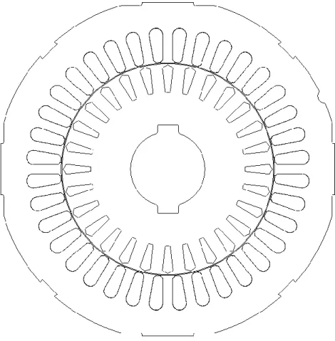
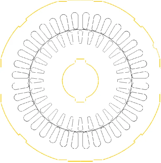
The first step of the simulation is to design the motor geometry, based on the constructive features described in section 2.1. Fig. 2.2 shows the two-dimensional motor geometry.

(28)

2.2.2. Assign Regions to Faces

Assigning regions to faces into the geometry is critical for the software to understand the composition of the motor. Fig. 2.3 shows the assignment of the faces, as well as the air and the infinite, while Fig. 2.4, Fig. 2.5 and Fig. 2.6 show the different faces position.

(29)

Fig. 2.4 – Faces of phase U (Flux2D).

Fig. 2.5 – Faces of phase V (Flux2D).

(30)

2.2.3. Mesh Creation

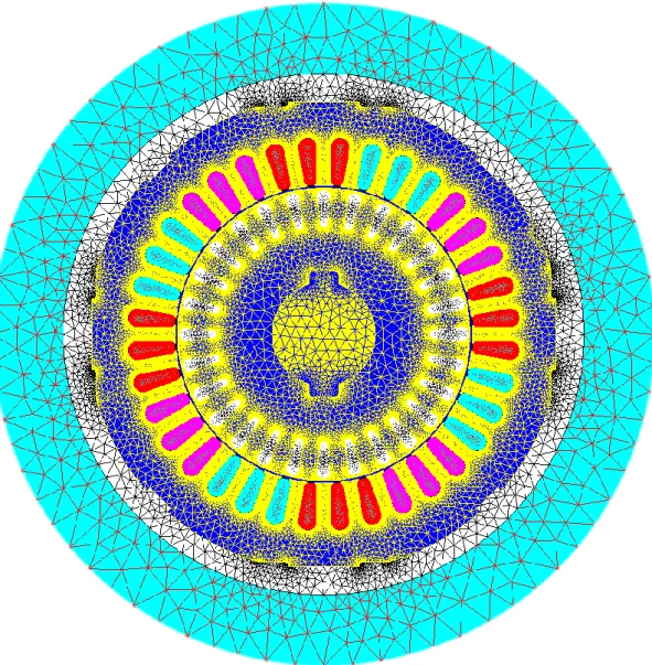
The software needs to mathematically recognize the entire construction, in order to be able to carry out the entire computational process. For this, it is necessary to create a mesh. This allows discretizing the geometry of the motor in small elements, by intermedium of nodal points, calculated approximately by computational methods. Through definitions such as deviation type, relaxation and point type, the software automatically adjusts all sets of elements according to the size and complexity of the faces, as can be seen in Fig. 2.7. The mesh is denser in the airgap area due to the need for accuracy.

(31)

2.2.4. Materials Definition

In order to initialize the electromagnetic simulation, the software requires the assignment of each material1_{to its respective face. For that, it is necessary to introduce their different} magnetic and electric properties, as well as their mass density.

Copper:  Magnetic properties:  Relative permeability = 1;  Electrical properties:  Resistivity = 1.72×10-8_[Ω.m];  Mass density = 8940 [kg/m3_]. Aluminum:  Magnetic properties:  Relative permeability = 1;  Electrical properties:  Resistivity = 2.7×10-8_[Ω.m];  Mass density = 2698.9 [kg/m3_]. Silicon Steel:  Magnetic properties:

 Initial relative permeability = 11368.21;  Saturation magnetization = 1.97 [T];  Knee adjusting coefficient = 2.89;  Electrical properties:

 Resistivity = 4.8×10-7_[Ω.m];  Mass density = 7650 [kg/m3_].

___________________________

1 _{Aluminum and copper parameters were taken from the website www.MATWEB.com. The} magnetic properties of silicon steel were provided by WEG and the remaining parameters, of this material, were taken from an identical material presented in the library of the software.

(32)

After this, the materials are inserted in their respective faces, but not every face needs a material, since the software already has the option “air or vacuum”, for faces such as infinity, air, air-gap and insulation. The shaft is defined as inactive, because this is one of the model boundary regions, as it will be seen later. The remaining faces are composed of the materials previously presented. Stator and rotor are made of silicon steel, the rotor bars are made of injected aluminum and the stator coils are made of copper. This is shown in Table 2.1.

Table 2.1 – Association of the material to its respective face.

Face Region Type Associated Material

Infinite Air or vacuum -

Air Air or vacuum -

Stator Magnetic non conducting Silicon steel

Coils Coil conductor Copper

Coil Insulation Air or vacuum -

Air-gap Air or vacuum -

Rotor Magnetic non conducting Silicon steel

Rotor Bars Solid conductor Aluminum

Shaft Inactive -

2.2.5. Mechanical Sets

As this is a model of an induction motor, it needs to rotate, so the software needs to simulate the rotation movement. In order to do that, it is necessary to introduce two mechanical sets, so that the software can distinguish the fixed part from the moving part. This way it is possible to simulate the rotation produced by the interaction of the rotating field of the stator with the one originated from the induced currents in the rotor bars.

The fixed part corresponds to every face that does not move. On the other hand, the rotational part corresponds to every face that rotates. The rotational part is dependent on the slip value, which is the input variable of the simulation scenario. Table 2.2, shows the mechanical set of each face.

Table 2.2 – Mechanical set of each face.

Face Mechanical Set

Infinite Fixed

Air Fixed

Stator Fixed

Coils Fixed

Coil Insulation Fixed

Air-gap Fixed

Rotor Rotational

Rotor Bars Rotational

(33)

2.2.6. Boundary Regions

Boundary regions are required for the correct simulation of the motor behavior. They define the work area of the electromagnetic simulation. These regions were already selected, because they can be selected automatically, using the infinite and defining the shaft as inactive. In this case the boundary lines are the infinite and the exterior of the shaft, as shown in Fig. 2.8.

Fig. 2.8 – Boundary lines – Electromagnetic simulation (Flux2D).

2.2.7. Electric Circuit

The induction motor needs an associated electric circuit, but in this software it has to be different from the equivalent circuit that is usually seen. This electric circuit needs the voltage values per phase, stator resistance and stator inductance values per phase, end rings values of

(34)

resistance and inductance, as well as the number of rotor bars. Its configuration can be seen in Fig. 2.9.

Fig. 2.9 – Electric circuit scheme (Flux2D).

The voltage value can be found in the rating plate of the induction motor. As the stator winding is connected in star, the line voltage is 400 V while the phase voltage is about 230 V.

Since this motor was rewound, the stator resistance value per phase present on the rating plate is not valid for the present modeling. The new value was measured between each two phases of the motor by using a multimeter, but this time at 21ºC, since this will be the initial temperature of the simulations. The results of each phase were: 2.12 Ω, 2.09 Ω and 2.08 Ω. After these three measurements were made, an average of them was made and the result of 2.1 Ω was introduced into the electric circuit.

In order to find the value of the stator inductance per phase, it was necessary to calculate the parameters of the induction motor through the equivalent circuit. For this, two experimental tests were performed, one at no-load condition and another with blocked rotor. In both conditions the voltage, the current and the mechanical power values were took, in order to calculate the parameters of the equivalent circuit. It was not possible to know the resistance and the inductance values of the rotor end rings (RRER and LRER, respectively), so, by iterative means, it was possible to adjust these parameters until a good correspondence have been found

(35)

Table 2.3shows the values of each component present in the electric circuit of the induction motor.

Table 2.3 – Values of the electric circuit components.

Components Values V [U] (0ᵒ) V [V] (120ᵒ) V [W] (-120ᵒ) 400 √3 ≈ 230.94 V RS [U, V, W] 2.1 Ω LS [U, V, W] 18.4 E-3 H

Squirrel Cage (28 bars) RRER=5.1987 E-6 Ω _{LRER=1 E-9 H}

After the electric circuit has been defined, it is possible to connect some faces with some of the circuit components, in particular the stator coils and the rotor bars, as can be seen in Table 2.4 and Table 2.5.

Table 2.4 – Assignment of the components to the coils.

Face Component Turn number Orientation

Coil [U1] R_U 6 × 36 Positive

Coil [U2] R_U 6 × 36 Negative

Coil [V1] R_V 6 × 36 Positive

Coil [V2] R_V 6 × 36 Negative

Coil [W1] R_W 6 × 36 Positive

Coil [W2] R_W 6 × 36 Negative

Table 2.5 – Assignment of the components to the bars.

Face Conductor type Associated conductor

Bar 1 Circuit (Squirrel Cage) Bar_1

… … …

Bar 28 Circuit (Squirrel Cage) Bar_28

2.2.8. Solving Scenario

Finally, it is necessary to carefully create a solving scenario, because it is necessary to have as many points as possible, to be able to visualize with big precision the motor behavior in steady state, but at the same time use as less points as possible, so that the simulation can run sufficiently fast. So, it is necessary to find an intermediate set of points, so that the simulation can be fast but also precise. These are presented in Table 2.6.

As the interest is focused on taking the losses values under rated conditions, it was necessary to look up for the associated rated slip point. Knowing that this is a four-pole machine and its

(36)

rated speed is 1435 rpm at a frequency of 50 Hz, the equations (4) and (5) were used to calculate the rated slip. The result was about 0.0433, so this will be the value used from now on. Ns= f×60 p (4) sn= ns-nn n_s (5)

Table 2.6 – Solving scenario – steady state.

Control Parameter

Lower Limit

Higher

Limit Method Value

Slip 0.01 0.1 List of _steps 0.01; 0.02; 0.03; 0.0433; 0.05; 0.06; _{0.07; 0.08; 0.09; 0.1} 0.1 0.5 Step value 0.01 0.5 1 Step value 0.1

2.2.9. Results Analysis

Current:

(37)

In Fig. 2.10the three-phase currents are presented as a function of the slip, where it is possible to see that each phase starts with a high current value and drops while slip decreases. This high current value is completely normal because in the motor starting the current values can reach about eight times the value of the rated current [38]-[39]. They should be equal, but during the starting period they are not equal. That happens due to the random starting relative position between rotor and stator. While the stator slots are 36 and the number of poles 4, the number of rotor bars is 28 which is not divisible by 3. This implies rotor impedance per phase different for the three phases. While the motor rotates, all the current values tend to reach the same value. Reaching the rated condition (at the rated slip), it can be seen that the current value is equal to the one found on the motor nameplate (4.56 A).

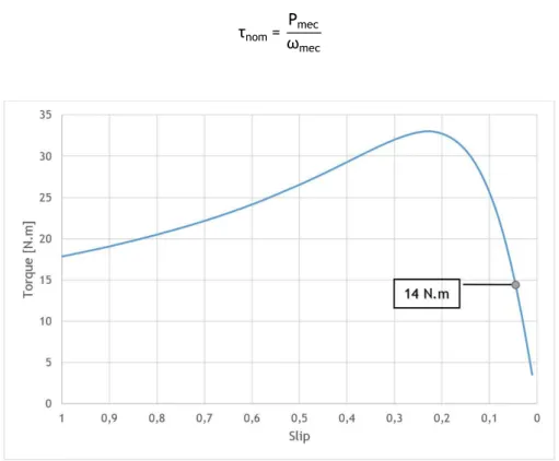
Torque:

Fig. 2.11 shows the torque variation curve as a function of the slip, where the rated operating point is being evidenced. In order to verify that the simulation results are close to the expected, it is necessary to calculate the torque, at rated condition. The equations (6) and (7) were used to calculate that value at rated condition, where the rated velocity is 1435 rpm and the mechanical power is 2.2 kW (values found in the motor nameplate). The calculated value was 14.64 N.m. ωmec = 2π × nn 60 (6) τnom = Pmec ωmec (7)

(38)

The results show that, for rated slip operation, the motor develops a torque of 14 N.m. There is a slightly difference between the simulation and the calculated value. This was expected since the motor was rewound, so it is possible to say that this is a quite good result.

Mechanical Power:

The variation of the mechanical power as a function of the slip is represented in Fig. 2.12, as well as the rated condition point. Equation (8) was used, in order to calculate the mechanical power.

Pmec = τ×ω (8)

Fig. 2.12 – Mechanical power as a function of the slip (Flux2D).

It is possible to observe that the mechanical power, at the rated operating point, did not reach the value found in the motor nameplate (2.2 kW), because the torque did not reach the expected value either. So, if the torque is slightly lower than expected, the mechanical power will also be slightly lower.

2.2.10. Losses Calculation

After an analysis of the results, as a function of the slip, it is necessary to focus on the rated slip point, in order to calculate the Joule and iron losses.

(39)

Joule losses:

The Joule losses (Pj) in the stator coils have a total of 158.21 W, which is the sum of the winding of the three phases of the induction motor. Individually the losses have the following values:

 Pj (U1) = 26.43 W;  Pj (U2) = 26.43 W;  Pj (V1) = 25.91 W;  Pj (V2) = 25.91 W;  Pj (W1) = 26.77 W;  Pj (W2) = 26.77 W;

The Joule losses in the rotor bars present a total of 55.43 W, which corresponds to 1.98 W for each bar.

Iron losses:

The software calculates the stator and the rotor iron losses through the Bertotti method [40]. This is based on the magnetic properties of the material, which in this case is the silicon steel. Its final result comes from the sum of two types of losses: hysteresis losses and eddy currents losses. However, it is necessary to give the program some coefficients so that the software can be able to calculate the iron losses values:

 kh (hysteresis losses constant);  σ (conductivity);

 ke (excess losses constant);  d (lamination thickness);  kf (stacking factor).

Some of these values are already known and others have to be taken from equation (9).

dPm = (kh × Bm2 × f + ( π2_{× σ × d}2 6 ) (Bm × f)2 + ke × (Bm × f) 3 2 ⁄_{× 8.67) × (}kf 𝜌) (9) where:  ρ = 7650 [kg/m3_] _{Mass density}

 σ = 2083333 [S/m] Conductivity (inverse of the

(40)

 d = 0.0005 [m] Lamination thickness

 kf = 0.97 Stacking factor

 Losses at:

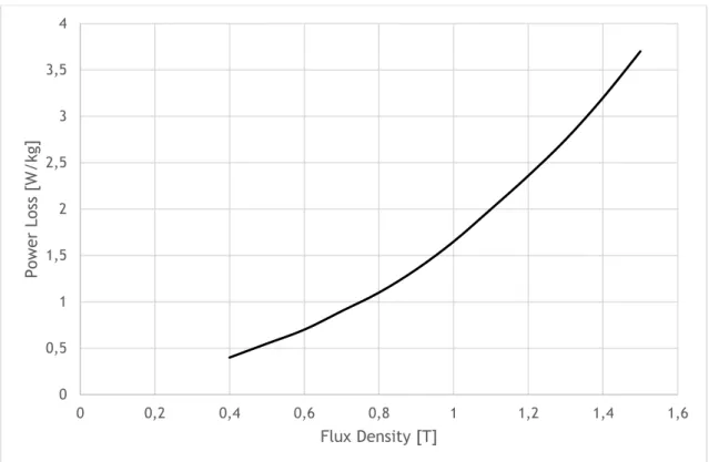
 Bm = 1T (50Hz)  dPm = 1.7 [W] Bm Peak value of magnetic flux density  Bm = 1.5T (50Hz)  dPm = 3.7 [W] dPm Losses in the peak value of the

magnetic flux density

Losses in the peak value of the magnetic flux density were taken from the manufacturer datasheet, Fig. 2.13.

Fig. 2.13 – Power loss curve characteristic of silicon steel as function of the peak flux density (WEG courtesy).

With all these values it was possible to solve equation (9), which resulted on ke ≈ 0.79 and kh ≈ 177.55. After having all these values, the software was able to calculate the iron losses of both stator and rotor. These results can be seen in Table 2.7.

Table 2.7 – Stator and rotor iron losses.

Losses Stator [W] Rotor [W]

Hysteresis 19.184 0.008 Eddy Currents 4.630 0.000 Total 23.814 0.008 0 0,5 1 1,5 2 2,5 3 3,5 4 0 0,2 0,4 0,6 0,8 1 1,2 1,4 1,6 Po w er Lo ss [ W /kg ] Flux Density [T]

(41)

2.3. Thermal Simulation

In this section, it was used the same structure also used for the electromagnetic simulation shown in Fig. 2.3 of the subsection 2.2.2. However, the “infinite” and “air” faces were removed and all the mechanical sets were also deleted, since none of them are relevant to the thermal study.

This thermal simulation is made along the time, so it is no longer a steady state simulation; instead it is a transient state simulation, where were used the losses calculated on steady state electromagnetic simulation.

Since this is a thermal simulation, it is necessary to add thermal properties of the materials. It is also necessary to add new materials2_{, which are related to the air-gap and the stator coils} insulation. Cooper:  Thermal Conductivity = 388 [W.m-1_.ºC-1_];  Thermal Inertia = 3441900 [J.m-3_.ºC-1_]. Aluminum:  Thermal Conductivity = 210 [W.m-1_.ºC-1_];  Thermal Inertia = 2429010 [J.m-3_.ºC-1_]. Silicon Steel:  Thermal Conductivity = 39 [W.m-1_.ºC-1_];  Thermal Inertia = 3800000 [J.m-3_.ºC-1_]. Air-gap:  Thermal Conductivity = 0.03 [W.m-1_.ºC-1_];  Thermal Inertia = 1214.4 [J.m-3_.ºC-1_];  Mass Density = 1.18415 [Kg/m3_]. ___________________________

(42)

Insulation:

 Thermal Conductivity = 0.083 [W.m-1_.ºC-1_];  Thermal Inertia = 1456000 [J.m-3_.ºC-1_];  Mass Density = 680 [Kg/m3_].

Table 2.8 presents the face configurations necessary for the thermal simulation, where the respective material and the respective losses can be found, calculated in subsection 2.2.10.

Table 2.8 – Faces configuration for thermal simulation.

Face Material Losses [W]

Stator Silicon Steel 23.81

Coil [U1] Cooper 26.43 Coil [U2] Cooper 26.43 Coil [V1] Cooper 25.91 Coil [V2] Cooper 25.91 Coil [W1] Cooper 26.77 Coil [W2] Cooper 26.77

Coil Insulation Insulation -

Air-gap Air-gap -

Rotor Silicon Steel 0.08

Each Rotor Bar Aluminum 1.98

Shaft - -

As also seen in the steady state electromagnetic simulation, it is necessary to introduce boundary regions. These can be seen in Fig. 2.14, where two boundary lines are represented, each one belonging to the outer stator and the inner rotor. Both lines depend on convection and radiation coefficients. These coefficients are fundamental elements in the study, since they define the behavior inside and outside of the boundary regions. However, the convection coefficient is different for each boundary line. This is due to the fact that there is not convection inside the rotor, since the boundary line is attached to the shaft. This is a zone that the ventilation cannot enter. In the exterior of the stator there is a forced convection that typically assumes values between 20-300 W/m2_{K. Therefore, the convection value was adjusted} for a room temperature of 21ᵒC.

(43)

Fig. 2.14 – Boundary lines – Thermal simulation (Flux2D).

2.3.1. Thermal Simulation Results

In this subsection, the thermal results obtained in the two-dimensional simulation will be presented. This thermal simulation had a duration of 10000 seconds (approximately 2h47m) and the beginning temperature was forced to be 21ᵒC.

In order to better understand the thermal behavior throughout the whole process, some intermediate steps are presented. Fig. 2.15presents the motor temperatures since the initial step (0 seconds) until the final step (10000 seconds). It can be seen that the temperatures between the rotor and the stator are quite similar at the beginning; however this starts to change somewhere between 1000 and 2000 seconds. In other words, the rotor starts becoming hotter than the stator between those values.

(44)

Fig. 2.15 – Motor thermal behavior at the time: a) 0s; b) 300s; c) 600s; d) 1000s; e) 2000s; f) 3000s; g) 4000s; h) 5000s; i) 6000; j) 10000s

(45)

More specific results about the motor thermal behavior for some simulation steps are following presented.

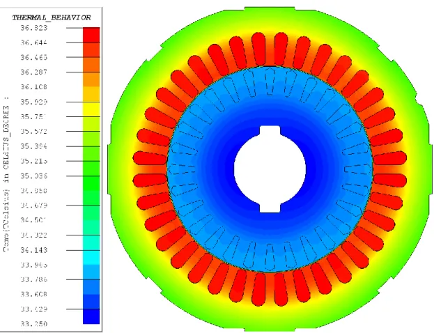
It can be seen in Fig. 2.16 that after 600 seconds (10 minutes), the motor is still in the initial heating process, although the temperatures have already started to increase. Now it can be seen that the rotor and stator temperatures are quite different. The lowest temperatures are located inside the rotor, near the shaft and the highest temperatures are located in the stator coils, having a difference about 3.5ᵒC. In the exterior of the stator are located the lowest stator temperatures, due to the air convection.

(46)

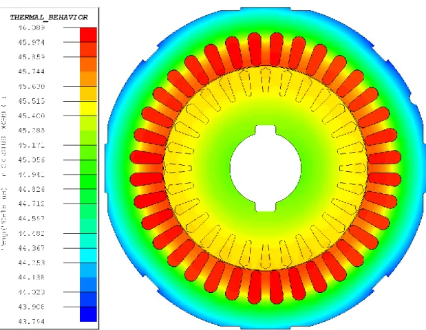
Fig. 2.17 shows that at the time 1200 seconds (20 minutes), the motor has already doubled its starting temperature distribution. Although the stator coils have the highest temperatures, the difference between these and the rotor bars is decreasing. At this point, those temperatures are already about 0.5ᵒC apart. It is also possible to see that the temperature differences between the lowest and the highest stator point have increased.

(47)

Then, after 2000 seconds (33 minutes and 20 seconds), it can be seen in Fig. 2.18, that due to the influence of the rotor bars, the rotor temperatures have already overtaken the stator coils temperatures.

(48)

At the time of 6000 seconds (1 hour and 40 minutes), it can be seen in Fig. 2.19 that the difference between the rotor and the stator temperatures continues to increase, being at this point about 12ᵒC apart. At this point the motor temperatures have almost stabilized.

(49)

Finally, after 10000 seconds (2 hours, 46 minutes and 40 seconds) the motor temperatures have already stabilized, and in Fig. 2.20 it can be seen that the motor thermal behavior has not changed much since the previous step (6000 seconds).

Having reached the steady-state operating point, it can be stated that the temperature difference between the rotor and the stator is about 13ᵒC, and the difference between the coolest and hottest stator points is about 5.5ᵒC.

(50)

(51)

Chapter 3

Transient State Condition

In this chapter, similar to what happened in Chapter 2 (Steady State Condition), two simulations will be made. Also here, the first one is the electromagnetic simulation followed by the thermal one. Some of the parameters are the same for both transient and steady state, so it is only necessary to describe the introduced changes. Parameters like the geometry, assignment of the faces, mesh, materials properties and boundary regions were the same, however the mechanical sets and the electric circuit were changed as well as a new solving scenario.

The most significant difference between the steady and transient state conditions is that in the steady state the focus is at only one operating point, there is no presence of time harmonics, the results are clear, that is why the simulation takes into account the slip and not the time. In transient state, it is expected to obtain a behavior closer to reality, because the simulation is over the time which means inclusion of the full harmonic index in the analysis. The transient state condition allows the analysis of the motor’s behavior along the time, but the existence of harmonics requires more careful data analysis. In this operation state, it is possible to observe the complete behavior of the motor, from the start-up until the rated operating point. Moreover, it can also be used to see other operating points or even faulty cases.

3.1. Electromagnetic Simulation

Firstly, the electromagnetic simulation will be carried out to calculate the Joule and iron losses of the motor. This simulation will be started by changing the mechanical sets, followed by the electric circuit and finally, as this is a time-based simulation, a new solving scenario will be created.

3.1.1. Mechanical Sets

The fixed part of the mechanical sets will stay unchanged, but the rotational part will be altered because in this simulation the slip will not be taken into account any more. As it was previously mentioned, this simulation will be made over time, so the software needs time dependent parameters others than the slip.

(52)

In this simulation it is possible to simulate the behavior of the induction motor with load coupling. Therefore, it is necessary to introduce values like torque, moment of inertia and initial speed. In this case the motor simulation will start with zero speed. The value of the moment of inertia was provided by WEG, so the following value will be used: 0.00897 kg.m2_. The torque value will change during the simulation. Initially, the motor will start at no-load condition (T = 0 N.m) and then will increase to the rated-load operation point (T =14 N.m). It is possible to see this illustrated in Fig. 3.1.

Fig. 3.1 – Introduced torque (Flux2D).

3.1.2. Electric Circuit

The electric circuit configuration in transient state electromagnetic simulation is very similar to the one in subsection 2.2.7, but there is a slight difference in the power supply voltage. An actual AC (Alternating Current) supply sinusoidal voltage with the individual phases 120º apart is supplied to the motor model. The changes can be found in Table 3.1.

Table 3.1 – Supply voltages of the electric circuit – transient state.

Component Equation V [U] 400 √3 × √2 × sin(2𝜋 × 𝑓𝑟𝑒𝑞𝑢𝑒𝑛𝑐𝑦 × 𝑡𝑖𝑚𝑒 + 0) V [V] 400 √3 × √2 × sin (2𝜋 × 𝑓𝑟𝑒𝑞𝑢𝑒𝑛𝑐𝑦 × 𝑡𝑖𝑚𝑒 + 2𝜋 3) V [W] 400 √3 × √2 × sin (2𝜋 × 𝑓𝑟𝑒𝑞𝑢𝑒𝑛𝑐𝑦 × 𝑡𝑖𝑚𝑒 − 2𝜋 3)

(53)

In the previous equations it is possible to observe that 400

√3 corresponds to the phase-to-ground

voltage value of the induction motor. This value needs to be multiplied by √2, because 400_√3 × √2 is the peak voltage value; in other words, it is the maximum amplitude of each phase. Finally, this value is multiplied by “sin”, responsible for making the supply voltage of each phase in a sinusoidal wave over the time. Each wave is also controlled by the supply frequency and by the angle of displacement 2𝜋

3 rad (120ᵒ).

3.1.3. Solving Scenario

In order to initiate the transient state electromagnetic simulation, it is necessary to create a new solving scenario. For this case it will be used a scenario of 0.5 seconds, like it is possible to see in Table 3.2.

Table 3.2 – Solving scenario – transient state.

Controlled Parameter Lower Limit Higher Limit Method Value

Time 0 0.5 Step value 5E-4

3.1.4. Results Analysis

For a better analysis of the results the following curves were extracted: supply voltages, supply currents, speed, torque and mechanical power, which are plotted in Figs. 3.2-3.7:

Supply Voltages:

(54)

Fig. 3.3 – Close view of the Fig. 3.2 (Flux2D).

Fig. 3.2 and Fig. 3.3 show that, as expected, the supply voltages are sinusoidal and with the individual phases 120º apart. Each one also has a peak value of 400_√3 × √2 ≈ 327 𝑉.

(55)

The starting currents can reach values about 8 times higher than their rated value [37]-[38], so the initial values of Fig. 3.4 are expected. After that, the current values decrease, because the motor is working at no-load condition (T = 0 N.m). At this working condition, the current values are about 2.85 A, but this is the peak value. The effectivevalue can be calculated by dividing it for √2. So the RMS value at no-load condition is about 2.02 A.

At the instant of 0.3 seconds, the load torque increases, and the current also increases, reaching the rated current value. The rated current value found in the motor nameplate is 4.56 A and the simulation value is 6.5

√2 ≈ 4.6 A. This value is slightly higher than expected due to the

presence of harmonics and because the material parameters are not exactly the same as for the experiment.

Speed:

Fig. 3.5 – Speed along 0.5 seconds (Flux2D).

As can be seen in Fig. 3.5 the motor starts from zero speed and then the speed starts increasing until it stabilizes at no-load condition, with a speed about 1499 rpm. From 0.3 seconds forward, the motor is working at rated-load condition. That means that the load torque has increased, and therefore the speed drops and stabilizes at 1435 rpm. This value is equal to the one found in the motor nameplate.

(56)

Torque:

Fig. 3.6 – Torque load along 0.5 seconds (Flux2D).

As it has been seen in Chapter 2, at the motor starting, or in other words, when the slip is close to 1, the torque reaches very high values. After that, it is possible to see in Fig. 3.6 that this value drops to a very low value, close to 0 N.m. At this point, the motor is working at no-load condition. At 0.3 seconds, the motor starts working at rated-load condition and it is possible to see the expected value (T = 14 N.m), previously defined in the subsection 3.1.1.

(57)

The mechanical power was taken from equation 8. That is why it is so similar to the torque.

It can be seen in Fig. 3.7 that the mechanical power has a high increase at the beginning, and after that, it becomes zero at the no-load condition. However, it has not stabilized yet, so some ripple can still be seen while the motor is working at no-load condition, although its value when it stabilizes would be about 90 W.

At 0.3 seconds, the motor starts working at rated-load condition, and as expected the mechanical power at this point is about 2.1 kW.

3.1.5. Losses Calculation

To proceed, it is necessary to extract the Joule and iron losses, in order to place them in the thermal simulation.

Joule Losses:

With a total of 151.18 W, the Joule losses in transient state condition are similar to those of the steady state simulation.

 Pj (U1) = 25.56 W;  Pj (U2) = 25.56 W;  Pj (V1) = 25.01 W;  Pj (V2) = 25.01 W;  Pj (W1) = 25.47 W;  Pj (W2) = 25.47 W;

The Joule losses in the rotor bars present a total of 59.52 W, which corresponds to 2.13 W for each bar.

Iron losses:

Bertotti method is a good method to calculate iron losses values for steady state simulations, although it is not that reliable for transient simulations, because it does not take into account the rotating losses. However, there is a more accurate method, named Loss Surface method (LS method). Although this is limited to the available materials, the required material parameters were found through its value of losses in the peak value of the magnetic flux density and through its thickness [40]. The iron losses results calculated by the LS model are presented in Table 3.3.

(58)

Table 3.3 – Iron losses at rated-load condition.

Stator [W] Rotor [W] Losses 23.65 1.18

In this case, the rotor iron losses have suffered an increase on their values due to the presence of harmonics that were not present in the steady state simulation. This increase will create a rise on the rotor final temperatures.

3.2. Analysis of Thermal Simulation Results

In order to validate the simulations results, they will be compared with the experimental results made available through the use of some thermal sensors, and considering a room temperature of 21ᵒC. Five PT100 sensors were used in the experimental tests, although it is not possible to compare all of them with the simulation results. This is because two of them are in a three-dimensional space and one is in the inner part of the motor frame, which is not presented in the two-dimensional model. The other two sensors were used to make the comparison between both tests. Their position can be seen in Fig. 3.8.

(59)

Fig. 3.9 shows the curve of each thermal sensor (PT100_2A and PT100_3) of both simulation and experimental tests throughout 10000 seconds. It is possible to see that the simulation results are quite close to the experimental results and their differences can be seen in Table 3.4.

Fig. 3.9 – Comparison between simulation and experimental thermal results.

Table 3.4 – Simulation and experimental thermal values after 10000 seconds.

Temperature Sensors [ᵒC] PT100_2A PT100_3 Experimental _67.66 _69.78 Simulation 67.64 69.66 20 25 30 35 40 45 50 55 60 65 70 0 2000 4000 6000 8000 10000 Te mpe ra tur e [ᵒC ] Time [s]

(60)

(61)

Chapter 4

Supply Voltage Unbalances

A three-phase induction motor is called balanced if the three-phase voltages and currents have the same amplitude and are phase-shifted by 120ᵒ with respect to each other. If either or both of these conditions are not gathered, the system is called unbalanced.

4.1. Amplitude Unbalance in Supply Voltages

Significant amplitude unbalance in supply voltages is not a usual fault, but can happen under some conditions. Following, are some of the more known common causes [41]:

 Defects in the power circuit connections;  Unmatched impedance on transformer banks;

 Unequal impedance in conductors of power supply wiring;  Unbalanced distribution of singe-phase loads;

 Malfunctioning of the equipment.

Regarding voltage unbalances it is required to touch some important aspects, related to the quantification of voltage unbalance, the unbalance caused in the currents and the percentage of temperature variation.

The quantification of voltage unbalance can be obtained by four different methods given by four different entities: National Equipment Manufacturers Association (NEMA), IEEE, International Electrotechnical Commission (IEC) and CIGRÉ (from the French – Conseil International des Grands Réseaux Électriques) [42]-[43]. Although four different definitions exist, only two will be used further to compare the results, because these are the most widespread in the literature.

The definition according to NEMA suggests the difference between the most deviated value and the average voltage value [8], [42]-[45]. Equation (10)can determine the percentage of voltage unbalance (PVU).