Leandro Félix Demuner , Diana Suckeveris , Julian Andrés Muñoz , Vinicius Camargo Caetano(1), Cesar Gonçalves de Lima(1),
Daniel Emygdio de Faria Filho(1) and Douglas Emygdio de Faria(1)
(1)Universidade de São Paulo (USP), Faculdade de Zootecnia e Engenharia de Alimentos, Avenida Duque de Caxias Norte, no 225, CEP 13635-900 Pirassununga, SP, Brazil. E-mail: leodemuner@usp.br, julianmunoz@usp.br, vinicius.usp.email@gmail.com, cegdlima@usp.br, fariafilho@usp.br, defaria@usp.br (2)USP, Escola Superior de Agricultura Luiz de Queiroz, Avenida Pádua Dias, no 11, CEP 13418-900 Piracicaba, SP, Brazil. E-mail: diana.usp@usp.br
Abstract – The objective of this work was to investigate adjustments of the Gompertz, Logistic, von Bertalanffy, and Richards growth models, in male and female chickens of the Cobb 500, Ross 308, and Hubbard Flex lines. Initially, 1,800 chickens were randomly housed in 36 pens, with six replicates per lineage and sex, fed ad libitum with feed according to gender, and bred until 56 days of age. Average weekly body weight for each line and sex was used to estimate model parameters using the ordinary least squares, weighted by the inverse variance of the body weight and weighted with a first-order autocorrelated error structure. Weighted models and weighted autocorrelated error models showed different parameter values when compared with the unweighted models, modifying the inflection point of the curve and according to the adjusted coefficient of determination, and the standard deviation of the residue and Akaike information criteria exhibited optimal adjustments. Among the models studied, the Richards and the Gompertz models had the best adjustments in all situations, with more realistic parameter estimates. However, the weighted Richards model, with or without ponderation with the autoregressive first order model AR (1), exhibited the best adjustments in females and males, respectively.
Index terms: autocorrelated errors, autoregressive model, poultry science, homogeneity of variance, mathematical model, weighting structures.
Ajuste de modelos de crescimento em frangos de corte
Resumo – O objetivo deste trabalho foi investigar os ajustes dos modelos de crescimento Gompertz, Logístico, von Bertalanffy e Richards em frangos fêmeas e machos das linhagens Cobb 500, Ross 308 e Hubbard Flex. Foram inicialmente utilizados 1.800 frangos, alojados aleatoriamente em 36 unidades experimentais, com seis repetições por linhagem e sexo, alimentados à vontade com ração, de acordo com o gênero, e criados até 56 dias de idade. A partir do peso vivo médio semanal de cada linhagem e sexo, realizou-se a estimação dos parâmetros dos modelos, por meio dos mínimos quadrados ordinários, ponderados pelo inverso da variância do peso e ponderados com estrutura de erros autocorrelacionados de primeira ordem. Modelos ponderados e modelos ponderados com autocorrelação apresentaram valores diferentes dos parâmetros comparados aos modelos não ponderados, mudando o ponto de inflexão da curva e de acordo com o coeficiente de determinação ajustado, e o desvio padrão do resíduo e os critérios de informação de Akaike apresentaram os melhores ajustes. Entre os modelos estudados, os de Richards e Gompertz resultaram nos melhores ajustes em todas as situações, com as estimativas mais reais dos parâmetros. Porém, o modelo ponderado de Richards, com ou sem ponderação com o modelo autorregressivo de primeira ordem AR (1), apresentou os melhores ajustes em fêmeas e machos, respectivamente.
Termos para indexação: erros autocorrelacionados, modelo autorregressivo, avicultura, homogeneidade da variância, modelos matemáticos, estruturas de ponderação.
Introduction
The current lineages of broiler chickens are a result of successful selection programs to achieve
rapid growth, improvements in body conformation, and a consequent reduction in animal slaughter age
(Zuidhof, 2014). An essential element to obtain these
performance of broiler chickens by adjusting growth curves. These curves arise from mathematical models that synthesize the development of the animal, in three or four parameters, evaluating the responses of the treatments over time, identifying the younger and heavier animals in a given population (Freitas, 2005).
Therefore, studying the selection of the optimal function for growth modeling is an essential step in the elaboration of production models. According to
Thornley & France (2007), the most applied curves
for bird development are Brody, Logistic, Gompertz, and von Bertalanffy; all of which are special cases of
Richard’s curve (Mohammed, 2015).
Modeling in animal production has a fundamental role in helping to maximize the system by producing high-precision estimates. This estimation depends on the non violation of statistical assumptions and can produce imprecise results, especially in cases with few samples (Mazucheli et al., 2011).
When studying animal growth, the heterogeneity of variances may occur for weight in function of animal age due to the differences found between weightings. Lower variation is observed in the initial phase of the animal’s life, increasing with age due to cumulative
effects during animal development (Mazucheli et
al., 2011; Silva et al., 2011; Tholon et al., 2012). In addition to the different time variances, these repeated measures may be correlated with dependent residues between the observed ages (Aggrey, 2009; Harring &
Blozis, 2014).
The objective of this work was to investigate adjustments of the Gompertz, Logistic, von Bertalanffy, and Richards growth models, in male and female chickens of the Cobb 500, Ross 308, and Hubbard Flex lines.
Materials and Methods
The experiment was conducted according to Brazilian guidelines, based on the Federal Law No.
11,794 of October 8, 2008 (Brasil, 2008), and approved by the ethics committee on animal use (Ceua), process
No. 14.1.148.74.7. The work was carried out in the poultry laboratory of the Department of Animal
Sciences of Faculdade de Zootecnia e Engenharia de
Alimentos of Universidade de São Paulo.
The eggs used in the experiment were purchased
from a commercial flock of different batches of 40– 50 week-old Cobb 500 (Cobb), Ross 308 (Ross), and
Hubbard Flex (Hubbard) broiler breeders and were
sent to an industrial hatchery. Initially, 1,800 one-day-old chicks were used, 300 of each lineage and sex. The animals were vaccinated for Marek’s disease, separated by gender in the hatchery, and vaccinated via intraocular route against the Newcastle and Gumboro diseases at seven days of age.
The experiment began in a 5x32-m experimental
aviary with a concrete floor, with 2.5-m ceiling height,
containing two identical rooms with 18 boxes each,
which measured 2.47 m2. Fifty one-day-old chicks
were housed in each box, distributed in six treatments: male Cobb; female Cobb; male Ross; female Ross; male Hubbard; female Hubbard, using a completely randomized design, containing six replicates per
treatment, totaling 36 experimental units (boxes). Wood shaving beddings were used, as well as
nipple drinkers and tubular feeders, according to the different stages of rearing and number of animals. Regarding heating for the birds in the pre-initial phase
of development, infrared lamps (250 W) and gas bells
were installed in the corridors. The adopted lighting program was of 23 hours of light + 1 hour of dark, from the second day of life of the chicks, using a timer. The daily air temperature and relative humidity
were registered using a Hobo data logger (Onset
Computer Corporation, Bourne, MA, USA), which
recorded mean±standard deviation of temperature values of 25.02±3.74°C and relative air humidity of
70.94±12.65%.
Animal diets were formulated with corn and soybean meal in alingment with the recommendations for superior performance of female and male broiler
chickens, as proposed by Rostagno (2011). The diets
were provided in the following phases: pre-initial, from 1 to 7 days; initial, from 8 to 21 days; growth I, from 22 to 35 days; growth II, from 36 to 42 days; and
final, from 43 to 56 days (Table 1).
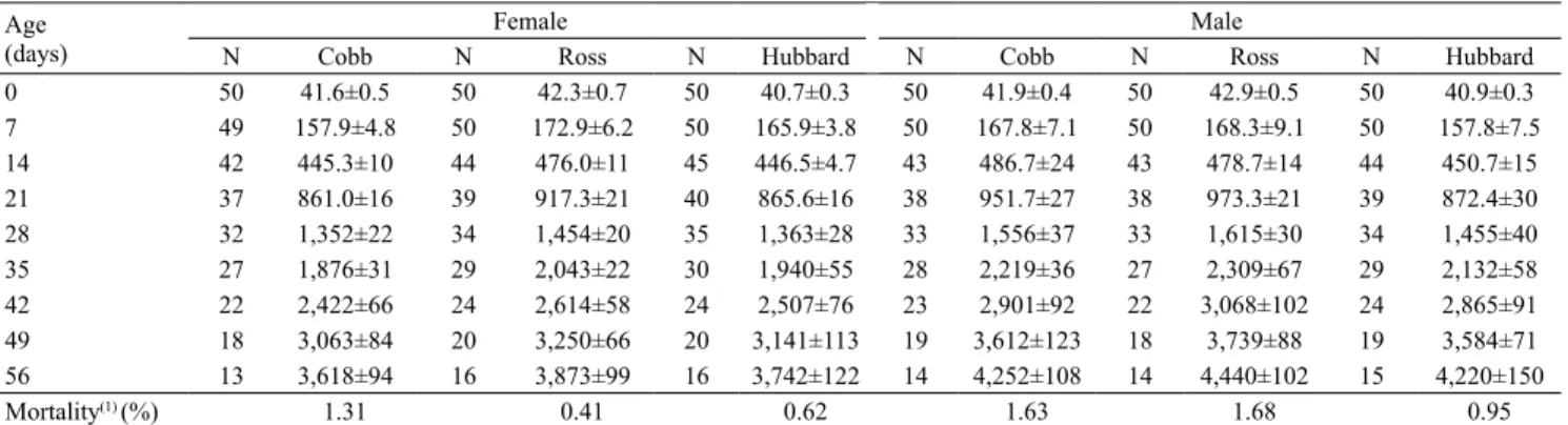
In order to obtain body weight (BW) for growth curve adjustment (Table 2), the birds of each box (experimental unit) were weighed weekly, and the mortalities (discard + natural death) and weights
of buckets and leftover feed from the feeder were registered for optimal control of the consumption of feed, which was offered freely throughout the experiment.
In addition to BW, other variables were estimated
regarding line and sex. Therefore, weekly sampling
Table 1. Composition percentage and calculated values for the broiler chicken experimental diets.
Ingredient
(%) (1–7 days)Pre-initial (8–21 days)Initial (22–35 days)Growth I (36–42 days)Growth II (43–56 days)Final
Male Female Male Female Male Female Male Female Male Female
Corn 53.59 55.09 57.62 56.13 59.15 61.45 63.44 65.63 65.31 67.29 Soybean meal 38.94 37.58 34.90 36.07 32.49 31.05 28.61 27.41 26.57 25.70 Soybean oil 2.903 2.639 3.441 3.723 4.622 4.140 4.522 4.072 4.900 4.457 Dicalcium phosphate 1.904 1.915 1.539 1.557 1.335 1.172 1.124 1.084 1.018 0.806 Calcitic limestone 0.911 0.911 0.935 0.944 0.888 0.877 0.794 0.625 0.745 0.659 Common salt 0.508 0.507 0.457 0.483 0.458 0.445 0.445 0.419 0.432 0.407 L-Lysine HCL 0.286 0.349 0.252 0.237 0.237 0.184 0.264 0.134 0.257 0.095
Methionine (MHA) 0.426 0.453 0.360 0.364 0.342 0.230 0.318 0.215 0.291 0.171 L-Threonine 0.116 0.146 0.085 0.081 0.072 0.037 0.076 0.000 0.067 0.000 Supplement(1) 0.400 0.400 0.400 0.400 0.400 0.400 0.400 0.400 0.400 0.400 Antioxidant(2) 0.013 0.013 0.013 0.013 0.013 0.013 0.013 0.013 0.013 0.013
Total 100 100 100 100 100 100 100 100 100 100
Energy and nutrients (%)
ME (kcal kg-1) 2,960 2,960 3,050 3,050 3,150 3,150 3,200 3,200 3,250 3,250
PB 22.40 22.00 21.20 20.80 19.80 19.20 18.40 17.80 17.60 17.10 Dig. lysine 1.324 1.341 1.217 1.201 1.131 1.057 1.060 0.933 1.006 0.862 Dig. methionin+cystine 0.953 0.965 0.876 0.864 0.826 0.722 0.774 0.681 0.734 0.629 Dig. methionine 0.652 0.670 0.588 0.581 0.555 0.456 0.519 0.430 0.489 0.386 Dig. threonine 0.861 0.871 0.791 0.780 0.735 0.687 0.689 0.608 0.654 0.585 Dig. tryptophan 0.253 0.246 0.237 0.231 0.218 0.211 0.198 0.192 0.187 0.183 Dig. arginine 1.417 1.379 1.334 1.302 1.231 1.193 1.226 1.092 1.065 1.044 Dig. valine 0.944 0.922 0.896 0.878 0.835 0.815 0.773 0.757 0.739 0.728 Dig. leucine 1.725 1.695 1.656 1.632 1.569 1.544 1.484 1.465 1.435 1.426 Dig. isoleucine 0.876 0.854 0.828 0.808 0.766 0.744 0.702 0.684 0.667 0.655 Calcium 0.920 0.920 0.841 0.831 0.758 0.711 0.663 0.587 0.614 0.528 Available phosphorus 0.470 0.470 0.401 0.396 0.354 0.322 0.309 0.274 0.286 0.246 Potassium 0.868 0.848 0.823 0.806 0.766 0.747 0.708 0.692 0.676 0.667 Sodium 0.220 0.220 0.210 0.200 0.200 0.195 0.195 0.185 0.190 0.180 Chlorine 0.354 0.354 0.339 0.325 0.325 0.317 0.318 0.303 0.310 0.296
(1)Vitamin/mineral premix: pre-initial diet – 2,000,000 IU kg-1 vitamin A (min.), 600,000 IU kg-1 vitamin D3 (min.), 3,000 IU kg-1 vitamin E (min.), 500
mg kg-1 vitamin K3 (min.), 600 mg kg-1 vitamin B1 (min.), 1,500 mg kg-1 vitamin B2 (min.), 1,000 mg kg-1 vitamin B6 (min.), 3,500 mcg kg-1 vitamin B12
(min.), 10 g kg-1 niacin (min.), 3,750 mg kg-1 pantothenic acid (min.), 250 mg kg-1 folic acid (min.), 86,600 g kg-1 choline (min.), 12,500 g kg-1 iron (min.),
17,500 g kg-1 manganese (min.), 12,500 g kg-1 zinc (min.), 24,950 g kg-1 copper (min.), 300 mg kg-1 iodine (min.), 50 mg kg-1 selenium (min.), and 3,750 mg
kg-1 virginamycine; initial diet – 1,750,000.00 IU kg-1 vitamin A (min.), 550,000.00 IU kg-1 vitamin D3 (min.), 2,750.00 IU kg-1 vitamin E (min.), 400.00
mg kg-1 vitamin K3 (min.), 500.00 mg kg-1 vitamin B1 (min.), 1,250.00 mg kg-1 vitamin B2 (min.), 750.00 mg kg-1 vitamin B6 (min.), 3,000.00 mcg kg
vitamin B12 (min.), 8,750.00 mg kg-1 niacin (min.), 3,250.00 mg kg-1 pantothenic acid (min.), 200.00 mg kg-1 folic acid (min.), 82.01 g kg-1 choline (min.),
12.50 g kg-1 iron (min.), 17.50 g kg-1 manganese (min.), 12.50 g kg-1 zinc (min.), 24.95 g kg-1 copper (min.), 300.00 mg kg-1 iodine (min.), 50.00 mg kg-1
selenium (min.), 25.00 g kg-1 monensin, and 7,500.00 mg kg-1 halquinol; growth diet – 1,500,000 IU kg -1 vitamin A (min.), (min.) 500,000 IU kg-1 vitamin
D3, 2,500 IU kg-1 vitamin E (min.), 400 mg kg-1 vitamin K3 (min.), 350 mg kg-1 vitamin B1 (min.), 1,000 mg kg-1 vitamin B2 (min.), 500 mg kg-1 vitamin
B6 (min.), 2,500 mcg kg-1 vitamin B12 (min.), 7,500 mg kg-1 niacin (min.), 2,750 mg kg-1 pantothenic acid (min.), 150 mg kg-1 folic acid (min.), 60,400 g
kg-1 choline (min.), 24,950 g kg-1 copper (min.), 12,500 g kg-1 iron (min.), 17,500 g kg-1 manganese (min.), 12,500 g kg-1 zinc (min.), 300 mg kg-1 iodine
(min.), 50 mg kg-1 selenium (min.), 7,500 mg kg-1 halquinol, and 15 g kg-1 salinomycin; and final diet – 1,250,000 IU kg -1 vitamin A (min.), 250,000 IU
kg-1 vitamin D3 (min.), 2,000 IU kg-1 vitamin E (min.), 400 mg kg-1 vitamin K3 (min.), 500 mg kg-1 vitamin B2 (min.), 1,250 mcg kg-1 vitamin B12 (min.),
5,000 mg kg-1 niacin (min.), 2,250 mg kg-1 pantothenic acid (min.), 31,900 g kg-1 cholin (min.), 12,500 g kg-1 iron (min.), 17,500 g kg-1 manganese (min.),
12,500 zinc (min.), 2,000 mg kg-1 copper (min.), 300 mg kg-1 iodine (min.), 50 mg kg-1 selenium (min.), and 2,500 mg kg-1 virginiamycin. (2)Feed Guard:
sample, was carried out in the first week (7 days of age) until the fifth week (35 days of age); and in the sixth week (42 days of age) until the eighth week (56 days of age), with four birds per sample. However, only
live chicken weights were used for model adjustment, and the change in the number of birds in the pen was
not significant (p>0.05) regarding weight of line and
gender; therefore, the variable bird number was not explored in the models.
The curves were adjusted and analyzed with the Proc
Model procedure of SAS, version 9.3 (SAS Institute Inc, Cary, NC, USA), which estimates the parameters
of nonlinear models using the Gauss-Newton iterative
process (Prado et al., 2013). The BW variance of each
age, line, and sex was calculated with the Proc Means also of the SAS software, by applying the inverse of the weight variances as a weighting factor using the
“Weight” option of the same software to verify the
effect of heteroscedasticity (Silva et al., 2011).
White’s test was used to detect heteroscedasticity
in the models, testing the equality of random error
variance. Moreover, Durbin-Watson’s (DW) test was
used to compare the null hypothesis that the residues are not correlated against the alternative hypothesis
that the residues have first order autocorrelation [AR(1)]. The performance of the models that were unweighted (UW), weighted (W), and weighted with AR(1) was assessed according to Motulsky & Christopoulos (2003) and Prado et al. (2013),
using the following equations for the adjusted
coefficient of determination (R2
adjusted), the standard
deviation of the residue (SDR), and the corrected
Akaike’s information criterion (AICc), respectively:
R n R
n q
2
2
1 1 1
adjusted = −
−
(
)
(
−)
−(
)
,in which R2= ×1
(
SSE SSTc)
is the non-adjustedcoefficient of determination and SSE is the sum of the
squares of the error; SSc is the sum of the total squares corrected by n, which is the number of weighings of live chicken; and q is the number of parameters in the model.
SDR= SSE
−
n q,
in which SSE is the sum of the squares of the error; n is the number of weighings of the live chicken; and q is the number of parameters in the model.
AICc n SQE
n q q q n q = +
(
+)
+(
−+(
)
(
++)
)
ln 2 1 2 1 2 ,
2
in which SQE is the sum of the squares of the residue; n is the number of weighings of live chicken; and q is the number of parameters in the model.
Akaike’s weight corresponds to the calculation of probability P
( )
= + − ( ) − ( ) exp exp , , 0 5 0 5 1 ∆ ∆ ,used in the selection of the most correct model (p>50%)
to be applied, based on the difference between the AICc of the models, ∆ =AICcb−AICca.
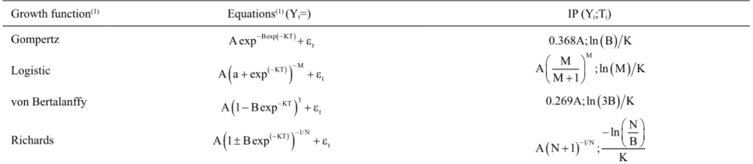
Table 2. Growth functions and inflection points (IP) used in the performed analyses.
Growth function(1) Equations(1) (Y
t=) IP (Yi;Ti)
Gompertz
Logistic
von Bertalanffy
Richards
(1)Gompertz, Logistic, and von Bertalanffy were adapted from Freitas (2005); while Richards was adapted from Tompić et al. (2011). A, asymptotic final
bodyweight; B, integration constant; K, maturity rate; M, (-1/n), i.e., the parameter that gives the curve its form; and, the residue in time t.
A B KT t exp− exp(− )+ ε
A a KT M
t
+
(
(− ))
− +exp ε
A B KT
t
1− 3
(
exp−)
+εA B KT
N t 1 1 ±
(
(− ))
+ − exp / ε0 368. A; ln( )B K
A M
M M K
M + ( )
1 ; ln
0.269A; ln(3B K)
A N N B K N + ( ) − −
1 1 ;
Results and Discussion
The mean weekly weights for each line and sex, as well as the mortality observed during the experiment, are shown in Table 3. Despite the weekly removal of birds, the mean body weight was close to the average recorded in the manuals of the respective lines. The accumulated mortality was 6.61%, with higher
mortality for males (4.26%) than females (2.35%).
Model assessment was carried out for each line and
gender, regarding unweighted (UW), weighted (W), and AR(1)-weighted structures. The adjustments for
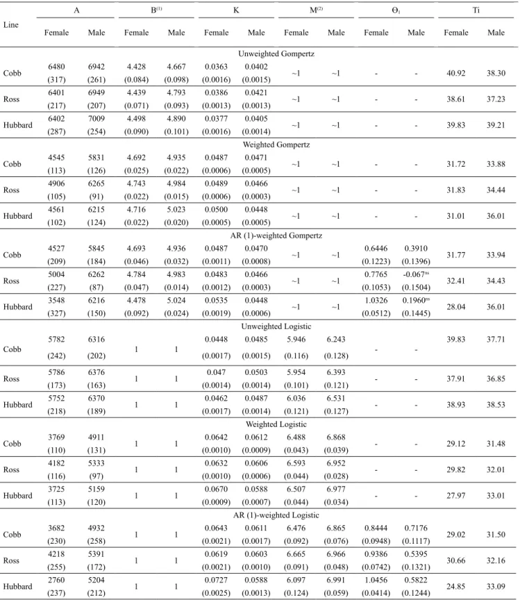
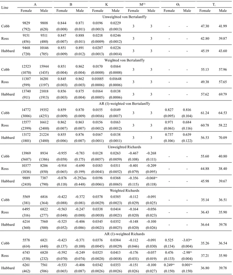
the Gompertz and Logistic models are shown in Table 4, and those for the von Bertalanffy and Richards models, in Table 5.
Following the incorporation of the structures in
the models, modifications in estimates regarding non-weighted models (traditional) were observed.
These changes followed the same pattern between
models (Tables 4 and 5), with the exception of the von
Bertalanffy model, with regard to: weight at maturity
in females (AGompertz = -29.75%; ALogistic = -35.54%;
ABertalanffy = 42.62%; and ARichards = -44.41%) and males
(AGompertz = -12.36%; ALogistic = -18.88%; ABertalanffy
= 86.87%; and ARichards = -12.74%); the integration
constant in females (BGompertz = 5.16%; BLogistic = 8.25%;
BBertalanffy = 0.87%; and BRichards = 44.06%) and males
(BGompertz = 4.15%; BLogistic = 8.59%; BBertalanffy = 1.73%;
and BRichards = 25.86%); and the maturity rate in females
(KGompertz = 32.44%; KLogistic = 42.56%; KBertalanffy =
-19.38%; and KRichards = 116.98%) and males (KGompertz
= 12.78%; KLogistic = 22.33%; KBertalanffy = -34.66%; and
KRichards = 24.98%).
The traditional Richards model displayed
convergence failure for parameters “B” and “N” in
Hubbard males, corroborating with the observations
made by Mota et al. (2015) and Silva et al. (2011). When incorporating the weighting and autocorrelation structures, it was difficult to approximate the values of
the additional autocorrelation parameter for Hubbard
male and female lines with the Richards model (Table 5), and for Ross and Hubbard male lines with the Gompertz model (Table 4).
According to Prado et al. (2013), parameter
estimation using the residues from the autoregressive
first order model AR (1) is not efficient, especially
when there is positive autocorrelation, as in the present study. Therefore, this may be more of a caution factor in choosing the best model, since the autocorrelation
parameter can be canceled.
The values of the parameters in the models with
incorporation of AR (1) in relation to the weighted
models presented little difference, with the exception of Hubbard females, which exhibited the lowest mean
value (± standard error) of “A” using the Gompertz model (3,548±327 g) and mainly using the Logistic model (2,760±237 g), which was below the final average weight (± standard error) observed at the end
of the experiment (3,742±49.95 g).
Traditional or structure incorporated Richards and
von Bertalanffy models estimated “unreal” values of weight at maturity for the lines and genders (Table 5), similar to what was observed by Mota et al. (2015) and
Table 3. Observed means±standard deviation for the number of birds per experimental unit (N) and mortality percentage of Cobb 500, Ross 308, and Hubbard Flex female and male broiler chickens.
Age
(days)
Female Male
Table 4. Mean estimates of the A, B, K, M, and Ti paremeters, as well as their standard errors (inside the parenthesis), for the unweighted, weighted, and the weighted with autocorrelated error (Ɵ1) Gompertz and Logistic models, regardingbody
weight measurements in Cobb 500, Ross 308, and Hubbard Flex female and male broiler chickens.
Line
A B(1) K M(2) Ɵ1 Ti
Female Male Female Male Female Male Female Male Female Male Female Male
Unweighted Gompertz
Cobb 6480 6942 4.428 4.667 0.0363 0.0402 ~1 ~1 - - 40.92 38.30
(317) (261) (0.084) (0.098) (0.0016) (0.0015)
Ross 6401 6949 4.439 4.793 0.0386 0.0421 ~1 ~1 - - 38.61 37.23
(217) (207) (0.071) (0.093) (0.0013) (0.0013)
Hubbard 6402 7009 4.498 4.890 0.0377 0.0405 ~1 ~1 - - 39.83 39.21
(287) (254) (0.090) (0.101) (0.0016) (0.0014)
Weighted Gompertz
Cobb 4545 5831 4.692 4.935 0.0487 0.0471 ~1 ~1 - - 31.72 33.88
(113) (126) (0.025) (0.022) (0.0006) (0.0005)
Ross 4906 6265 4.743 4.984 0.0489 0.0466 ~1 ~1 - - 31.83 34.44
(105) (91) (0.022) (0.015) (0.0006) (0.0003)
Hubbard 4561 6215 4.716 5.023 0.0500 0.0448 ~1 ~1 - - 31.01 36.01
(102) (124) (0.022) (0.020) (0.0005) (0.0005)
AR (1)-weighted Gompertz
Cobb 4527 5845 4.693 4.936 0.0487 0.0470 ~1 ~1 0.6446 0.3910 31.77 33.94
(209) (184) (0.046) (0.032) (0.0011) (0.0008) (0.1223) (0.1396)
Ross 5004 6262 4.784 4.983 0.0483 0.0466 ~1 ~1 0.7765 -0.067
ns
32.41 34.43
(227) (87) (0.047) (0.014) (0.0012) (0.0003) (0.1053) (0.1504)
Hubbard 3548 6216 4.478 5.024 0.0535 0.0448 ~1 ~1 1.0326 0.1960
ns
28.04 36.01
(327) (150) (0.092) (0.024) (0.0019) (0.0006) (0.0512) (0.1445)
Unweighted Logistic
Cobb
5782 6316
1 1
0.0448 0.0485 5.946 6.243
-
-39.83 37.71
(242) (202) (0.0017) (0.0015) (0.116) (0.128)
Ross 5786 6376 1 1 0.047 0.0503 5.954 6.393 - - 37.91 36.85
(173) (163) (0.0014) (0.0014) (0.101) (0.121)
Hubbard 5752 6370 1 1 0.0462 0.0487 6.036 6.531 - - 38.93 38.53
(218) (189) (0.0017) (0.0014) (0.121) (0.127) Weighted Logistic
Cobb 3769 4911 1 1 0.0642 0.0612 6.488 6.868 - - 29.12 31.48
(110) (131) (0.0010) (0.0009) (0.043) (0.039)
Ross 4182 5333 1 1 0.0632 0.0606 6.593 6.952 - - 29.82 32.01
(116) (97) (0.0010) (0.0006) (0.044) (0.028)
Hubbard 3725 5159 1 1 0.0670 0.0588 6.507 6.977 - - 27.97 33.01
(113) (120) (0.0009) (0.0007) (0.044) (0.034) AR (1)-weighted Logistic
Cobb 3682 4932 1 1 0.0643 0.0611 6.476 6.865 0.8444 0.7176 29.02 31.50
(230) (258) (0.0021) (0.0017) (0.092) (0.076) (0.0948) (0.1117)
Ross 4218 5391 1 1 0.0619 0.0603 6.665 6.966 0.9386 0.5395 30.66 32.16
(255) (172) (0.0021) (0.0010) (0.091) (0.048) (0.0742) (0.1321)
Hubbard 2760 5204 1 1 0.0727 0.0588 6.097 6.991 1.0456 0.5822 24.85 33.09
(237) (212) (0.0025) (0.0013) (0.124) (0.059) (0.0414) (0.1244)
(1)Fixed b-value (1) regarding the Logistic model. (2)Value of m is approximately one (~1) for the Gompertz model. nsNonsignificant by the approximate
Table 5. Mean estimates of the A, B, K, M, and Ti parameters, as well as their standard errors (inside the parenthesis), for the unweighted, weighted, and weighted with autocorrelated error (Ɵ1)Richards and von Bertalanffy models regarding body
weight measurements in Cobb 500, Ross 308, and Hubbard Flex female and male broiler chickens.
Line A B K M
(1) Ɵ
1 Ti
Female Male Female Male Female Male Female Male Female Male Female Male Unweighted von Bertalanffy
Cobb 9829 9808 0.844 0.871 0.0196 0.0229 3 3 - - 47.30 41.99
(792) (628) (0.008) (0.011) (0.0013) (0.0013)
Ross 9151 9511 0.847 0.888 0.0218 0.0246 3 3 - - 42.80 39.87
(456) (480) (0.007) (0.011) (0.0009) (0.0012)
Hubbard 9468 10146 0.851 0.891 0.0207 0.0226 3 3 - - 45.19 43.60
(720) (705) (0.009) (0.012) (0.0013) (0.0014)
Weighted von Bertalanffy
Cobb 12523 15944 0.851 0.862 0.0170 0.0164 3 3 - - 55.13 57.96
(1070) (1435) (0.004) (0.004) (0.0008) (0.0008)
Ross 11307 16201 0.845 0.862 0.01885 0.01648 3 3 - - 49.38 57.65
(599) (1197) (0.003) (0.003) (0.0006) (0.0006)
Hubbard 13740 21018 0.856 0.875 0.0164 0.0138 3 3 - - 57.62 69.79
(911) (1913) (0.003) (0.004) (0.0005) (0.0006)
AR (1)-weighted von Bertalanffy
Cobb 14772 19352 0.859 0.870 0.0155 0.0149 3 3 0.827 0.816 61.24 64.53
(3006) (4251) (0.009) (0.009) (0.0016) (0.0017) (0.095) (0.104)
Ross 15577 16612 0.862 0.863 0.0156 0.0163 3 3 0.971 0.684 60.78 58.22
(2399) (2400) (0.007) (0.007) (0.0012) (0.0012) (0.061) (0.116)
Hubbard 13172 21224 0.855 0.876 0.0167 0.0138 3 3 0.737 0.639 56.53 70.09
(1801) (3480) (0.006) (0.007) (0.0011) (0.0011) (0.106) (0.122)
Unweighted Richards
Cobb 13969 8934 -0.955 -0.783 0.0128 0.0263 -0.467 -0.268 - - 55.60 40.80
(5607) (1386) (0.058) (0.175) (0.0057) (0.0059) (0.108) (0.111)
Ross 10377 8206 -0.914 -0.690 0.0183 0.0311 -0.401 -0.209 - - 44.88 38.40
(1836) (850) (0.065) (0.199) (0.0041) (0.0052) (0.079) (0.095)
Hubbard 9889 7387 -0.876 -0.292ns 0.0196 0.0368 -0.356 -0.068
ns
- - 45.98 39.67
(2418) (790) (0.118) (0.448) (0.0061) (0.0065) (0.115) (0.118) Weighted Richards
Cobb 5569 6816 -0.422 -0.372 0.0378 0.0385 -0.112 -0.091 - - 35.14 36.51
(381) (364) (0.088) (0.081) (0.0029) (0.0023) (0.029) (0.025)
Ross 6495 6822 -0.563 -0.247 0.0338 0.0414 -0.164 -0.056 - - 36.43 35.90
(316) (277) (0.048) (0.088) (0.0018) (0.0021) (0.020) (0.023)
Hubbard 6214 7560 -0.525 -0.406 0.0345 0.0352 -0.148 -0.100 - - 36.64 39.78
(360) (500) (0.052) (0.086) (0.0021) (0.0025) (0.020) (0.026) AR (1)-weighted Richards
Cobb 5578 6821 -0.423 -0.371 0.0376 0.0384 -0.112 -0.091 0.525 -3.03
ns
35.26 36.54
(614) (448) (0.137) (0.100) (0.0045) (0.0029) (0.046) (0.030) (0.134) (0.004)
Ross 6743 6820 -0.592 -0.249 0.0325 0.0413 -0.176 -0.057 0.476 -2.98
ns
37.21 35.90
(538) (232) (0.070) (0.074) (0.0028) (0.0018) (0.031) (0.019) (0.133) (0.004)
Hubbard 6261 7561 -0.533 -0.406 0.0342 0.0353 -0.151 -0.100 0.249
ns 0.001ns
36.80 39.78
(462) (506) (0.065) (0.087) (0.0026) (0.0026) (0.026) (0.027) (0.150) (0.150)
Drumond et al. (2013), while using the traditional von
Bertanlaffy model on quails. According to Fitzhugh Jr.
(1976), to determine the method of choice of the adjusted growth curve, the model must have an optimum fit
of data, retain correct biological interpretation, and
present no difficulty in data convergence.
Gbangboche et al. (2008) highlighted that model
choice affects parameter estimation, affecting the
inflection point (IP) of the curve, which is an important
economic indicator in animal production. It is known that the point of the von Bertalanffy model is close to
26.9% of the value of “A” and the Gompertz model has an IP of the curve close to 36.8% of “A”. However, the
Logistic and Richards models vary according to the
“M” (1/N) of the curve (Table 3).
The variations in model parameters affected the
curve inflection day (Ti) due to the strong correlation between them (Eleroğlu et al., 2014), which contributed to greater precocity among females (TiGompertz = -21.70%;
TiLogistic = -26.47%; and TiRichards = -24.93%) than males
(TiGompertz = -9.04%; TiLogistic = -14.55%; and TiRichards =
-5.57%), when comparing the traditional models to the modified ones. The von Bertanlaffy model was
an exception since it exhibited elevated values of
“A” and curve IP for females (TiBertalanffy = 26%) and
for males (TiBertalanffy = 50.53%), when weighting and
autocorrelation were incorporated.
In Table 6 and 7, the values regarding the quality of
the adjustments (R2adj, SDR, and AICc) of the models,
tests of heteroscedasticity (White test), and the test for error independents (Durbin-Watson test) are shown,
according to line and gender.
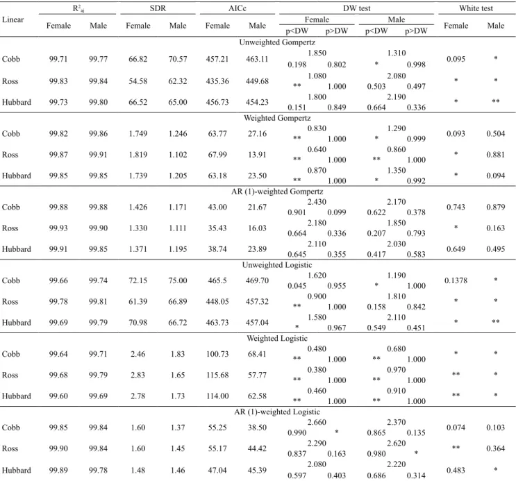
The adjusted coefficients of determination (R2adj)
for the models in the present study were close to one hundred, noting that performance was enhanced when a structure was incorporated. In this case, caution should be taken when evaluating the quality of the adjustment since R2
adj is not a good differentiator in the choice of
models, considering that they are high and close (Silva
et al., 2011; Drumond et al., 2013). According to Tholon
et al. (2012), multicollinearity, in this case, may occur
due to the high relationship between the dependent
variables of the model, not exhibiting any significance
in the regression coefficients.
As shown in Table 7 and 8, the SDR, regarding the weighted and autocorrelation-weighted models, was reduced from 95.88 to 98.36%, in comparison with the unweighted models. This result shows that there was less oscillation in the observed points of weight
in relation to the predicted mean when a structure was incorporated into the models.
Lower AICc estimates were verified in weighted
models, which were close to those found in the model that was weighted with autocorrelated errors. Therefore, choosing the optimal approach for model
adjustment was inconclusive.
Regarding the majority of the studied groups, the traditional models displayed heteroscedasticity
and error autocorrelations, according to the White and Durbin-Watson (DW) tests, in Tables 6 and 7,
respectively. When weighting was performed without
the AR (1) structure, homoscedasticity was observed
for all the studied groups using the Richards model, but with positive autocorrelation for Cobb females and
males (Table 7). In turn, when combining weighting and AR (1), there was an improvement in the adjustments
and error independence using the Gompertz, Logistic,
and Richards models, regarding female lines.
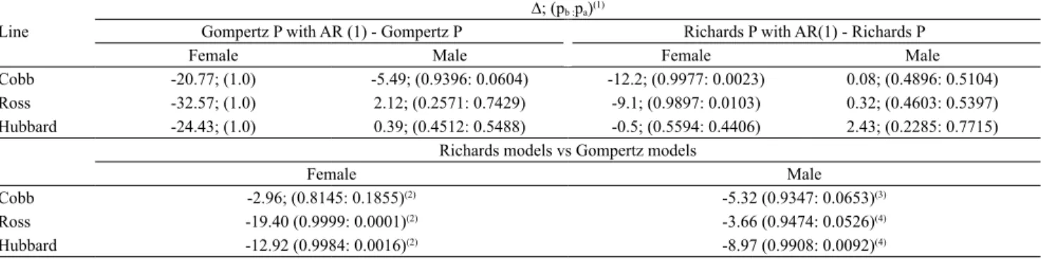
In order to avoid causing uncertainty to the researcher regarding the small differences described between the AICc of the models, the weight of AICc was calculated
(Prado et al., 2013). Due to optimal adjustments and
parameter interpretation, only the weighted and AR
(1)-weighted Gompertz and Richards models were compared (Table 8). Between these models, the combined structures were verified as being more correct (p>50%) in the female lines. In turn, regarding
the male lines, Cobb chickens were the most accurate
(p>50%) only for the AR (1)-weighted Gompertz
model, whereas, for Ross and Hubbard chickens, the
best performances (p>50%) were observed using the
Richards and Gompertz weighted models.
With regard to the outcome of the models, an alternative comparison was carried out (Table 8), this
time using the optimum models separately. As a result, the use of the Richards model, weighted with the AR
(1) structure, was more adequate for females (Cobb = 81.45%; Ross = 99.99%; Hubbard = 99.84%), and the
weighted Richards model was more appropriate for
males (Cobb = 93.47%; Ross = 94.74%; Hubbard = 99.08%).
Mazucheli et al. (2011), in a study on chicken
growth using the homoscedastic and heteroscedastic Gompertz model with independent errors, concluded that the weighted model was more appropriate than
the unweighted one. The authors verified less weight
precision regarding the statistical effect and studied factors, as in the current study.
In literature, different conclusions with respect to the adjustment of growth models in birds were reached. Tompić et al. (2011) obtained the best adjustments using the Richards and Gompertz growth models in broilers;
Yang et al. (2006) reported the von Bertalanffy model as the most accurate in Jinghai Yellow chicken; and Eleroğlu et al. (2014) had concluded that the Logistic model the best fit in growth of slow performance
chickens. However, despite the variety of existing growth models, one of the most recommended ones
Table 6. Mean adjustment assessment of the unweighted, weighted, and weighted with autocorrelated error Gompertz and Logistic models regarding body weight measurements in Cobb 500, Ross 308, and Hubbard Flex female and male broiler chickens, by way of the adjusted coefficient of determination (R2
aj), the standard deviation of the residue (SDR), the
corrected Akaike information criteria (AICc), the Durbin-Watson (DW) test, and the White test.
Linear
R2
aj SDR AICc DW test White test
Female Male Female Male Female Male Female Male Female Male
p<DW p>DW p<DW p>DW
Unweighted Gompertz
Cobb 99.71 99.77 66.82 70.57 457.21 463.11 1.850 1.310 0.095 * 0.198 0.802 * 0.998
Ross 99.83 99.84 54.58 62.32 435.36 449.68 1.080 2.080 * * ** 1.000 0.503 0.497
Hubbard 99.73 99.80 66.52 65.00 456.73 454.23 1.800 2.190 * ** 0.151 0.849 0.664 0.336
Weighted Gompertz
Cobb 99.82 99.86 1.749 1.246 63.77 27.16 0.830 1.290 0.093 0.504 ** 1.000 * 0.999
Ross 99.87 99.91 1.819 1.102 67.99 13.91 0.640 0.860 * 0.881 ** 1.000 ** 1.000
Hubbard 99.85 99.85 1.739 1.205 63.18 23.50 0.870 1.350 * 0.094 ** 1.000 * 0.992
AR (1)-weighted Gompertz
Cobb 99.88 99.88 1.426 1.171 43.00 21.67 2.430 2.170 0.743 0.879 0.901 0.099 0.622 0.378
Ross 99.93 99.90 1.330 1.111 35.43 16.03 2.180 1.850 * 0.163 0.664 0.336 0.207 0.793
Hubbard 99.91 99.85 1.371 1.195 38.74 23.89 2.110 2.030 0.649 0.495 0.645 0.355 0.417 0.583
Unweighted Logistic
Cobb 99.66 99.74 72.15 75.00 465.5 469.70 1.620 1.190 0.1378 * 0.045 0.955 * 1.000
Ross 99.78 99.81 61.39 66.89 448.05 457.32 0.900 1.810 * * ** 1.000 0.158 0.842
Hubbard 99.69 99.79 70.98 66.72 463.73 457.04 1.580 2.110 * ** * 0.967 0.549 0.451
Weighted Logistic
Cobb 99.64 99.71 2.46 1.83 100.73 68.41 0.480 0.680 * * ** 1.000 ** 1.000
Ross 99.68 99.79 2.83 1.65 115.68 57.77 0.380 0.970 ** * ** 1.000 ** 1.000
Hubbard 99.60 99.69 2.78 1.73 114.00 62.58 0.460 0.910 ** * ** 1.000 ** 1.000
AR (1)-weighted Logistic
Cobb 99.85 99.84 1.60 1.37 55.25 38.50 2.660 2.370 0.074 0.103 0.990 * 0.865 0.135
Ross 99.90 99.84 1.60 1.45 55.17 44.42 2.290 2.620 ** 0.364 0.837 0.163 0.980 *
Hubbard 99.89 99.78 1.48 1.46 47.04 45.39 2.080 2.220 0.483 * 0.597 0.403 0.686 0.314
has been the Gompertz model in its traditional form
(Freitas, 2005; Mazucheli et al., 2011; Drumond et al., 2013; Mohammed, 2015; Mota et al., 2015).
In the current study, the Gompertz model exhibited optimal interpretation and convergence of estimates in its traditional form, when compared to the
traditional Richards model. However, when weighted
or weighted with the AR (1) structure, the Richards model displayed superior fit and interpretation of
parameter estimates, showing that model selection may vary according to the data and the use of statistical properties.
Table 7. Mean adjustment assessment of the unweighted, weighted, and weighted with autocorrelated error von Bertalanffy and Richards models regarding body weight measurements of Cobb 500, Ross 308, and Hubbard Flex female and male broiler chickens, by way of the adjusted coefficient of determination (R2
aj), the standard deviation of the residue (SDR), the
corrected Akaike information criteria (AICc), the Durbin-Watson (DW) test, and the White test.
Line
R2
aj (%) SDR AICc DW test White test
Female Male Female Male Female Male Female Male Female Male
p<DW p>DW p<DW p>DW
Unweighted von Bertalanffy
Cobb 99.77 99.79 59.16 67.38 444.1 458.1 2.260 1.370 * * 0.752 0.249 * 0.996
Ross 99.88 99.84 45.65 60.77 416.06 446.96 1.400 2.220 * * 0.005 0.995 0.700 0.300
Hubbard 99.77 99.78 61.63 68.20 448.48 459.42 2.110 1.950 * * 0.555 0.445 0.319 0.682
Weighted von Bertalanffy
Cobb 99.68 99.66 2.293 1.953 93.01 75.71 0.620 0.660 ** ** ** 1.000 ** 1.000
Ross 99.86 99.66 1.881 2.103 71.61 83.69 0.540 0.740 ** ** ** 1.000 ** 1.000
Hubbard 99.80 99.70 1.977 1.713 76.99 61.50 0.660 0.850 ** ** ** 1.000 ** 1.000
AR (1)-weighted von Bertalanffy
Cobb 99.85 99.83 1.560 1.381 55.25 38.50 2.230 2.660 ** * 0.738 0.262 0.989 *
Ross 99.95 99.79 1.152 1.640 55.17 44.42 2.520 2.690 * * 0.970 * 0.991 *
Hubbard 99.89 99.80 1.444 1.390 47.04 45.39 2.130 2.260 * 0.563 0.581 0.419 0.746 0.254
Unweighted Richards
Cobb 99.77 99.79 58.86 67.81 444.8 460.1 2.300 1.390 * * 0.750 0.250 * 0.997
Ross 99.88 99.85 45.77 60.30 417.60 447.39 1.400 2.280 * * * 0.997 0.728 0.272
Hubbard 99.76 99.80 62.22 65.45 450.78 456.24 2.120 2.190 * ** 0.505 0.495 0.612 0.388
Weighted Richards
Cobb 99.86 99.89 1.553 1.114 52.21 16.27 1.060 1.610 0.168 0.942 ** 1.000 * 0.970
Ross 99.94 99.92 1.209 1.050 25.16 9.93 1.170 2.3 0.462 0.914 * 1.000 0.762 0.238
Hubbard 99.92 99.88 1.222 1.071 26.30 12.10 1.550 2.04 0.437 0.732 * 0.983 0.393 0.607
AR (1)-weighted Richards
Cobb 99.89 99.89 1.371 1.101 40.04 16.35 2.260 2.080 0.407 0.900 0.700 0.300 0.445 0.555
Ross 99.95 99.92 1.097 1.040 16.02 10.25 2.060 1.750 0.110 0.750 0.400 0.600 0.088 0.912
Hubbard 99.93 99.88 1.201 1.082 25.82 14.53 2.010 2.040 0.514 0.963 0.338 0.662 0.392 0.608
Conclusions
1. The incorporation of weighting and AR (1)
weighting structures into growth models modifies
the values of the parameters, and hampers the approximation of the autocorrelation parameter, showing that attention regarding statistical assumptions is necessary.
2. The weighted and AR (1)-weighted Richards
models show optimal properties in model selection for males and females, respectively.
Acknowledgments
To Coordenação de Aperfeiçoamento de Pessoal de
Nível Superior (Capes), for scholarship granted.
References
AGGREY, S.E. Logistic nonlinear mixed effects model for
estimating growth parameters. Poultry science, v.88, p.276-280, 2009. DOI: 10.3382/ps.2008-00317.
BRASIL. Lei nº 11.794, de 8 de outubro de 2008. Regulamenta o inciso VII do § 1º do art. 225 da Constituição Federal, estabelecendo
procedimentos para o uso científico de animais; revoga a Lei nº
6.638, de 8 de maio de 1979; e dá outras providências. Diário
Oficial da União, 9 out. 2008. Seção 1, p.1-2.
DRUMOND, E.S.C.; GONÇALVES, F.M.; VELOSO, R. de C.; AMARAL, J.M.; BALOTIN, L.V.; PIRES, A.V.; MOREIRA, J. Curvas de crescimento para codornas de corte. Ciência Rural, v.43, p.1872-1877, 2013. DOI: 10.1590/S0103-84782013001000023.
ELEROĞLU, H; YILDIRIM, A.; SEKEROĞLU, A.; ÇOKSÖYLER, F.N.; DUMAN, M. Comparison of growth curves
by growth models in slow–growing chicken genotypes raised
the organic system. International Journal of Agriculture and
Biology, v.16, p.529-535, 2014.
FITZHUGH JR., H.A. Analysis of growth curves and strategies
for altering their shape. Journal of Animal Science, v.42, p.1036-1051, 1976. DOI: 10.2527/jas1976.4241036x.
FREITAS, A.R. de. Curvas de crescimento na produção animal.
Revista Brasileira de Zootecnia, v.34, p.786-795, 2005. DOI:
10.1590/S1516-35982005000300010.
GBANGBOCHE, A.B.; GLELE-KAKAI, R.; SALIFOU, S.;
ALBUQUERQUE, L.G.; LEROY, P.L. Comparison of non-linear growth models to describe the growth curve in West African
Dwarf sheep. Animal, v.2, p.1003-1012, 2008. DOI: 10.1017/ S1751731108002206.
HARRING, J.R.; BLOZIS, S.A. Fitting correlated residual error
structures in nonlinear mixed-effects models using SAS PROC NLMIXED. Behavior Research Methods, v.46, p.372-384, 2014. DOI: 10.3758/s13428-013-0397-z.
MAZUCHELI, J.; SOUZA, R.M. de; PHILIPPSEN, A.S. Modelo de crescimento de Gompertz na presença de erros normais heterocedásticos: um estudo de caso. Revista Brasileira de
Biometria, v.29, p.91-101, 2011.
MOHAMMED, F.A. Comparison of three nonlinear functions for describing chicken growth curves. Scientia Agriculturae, v.9, p.120-123, 2015.
MOTA, L.F.M.; ALCÂNTARA, D.C.; ABREU, L.R.A.; COSTA, L.S.; PIRES, A.V.; BONAFÉ, C.M.; SILVA, M.A.; PINHEIRO, S.R.F. Crescimento de codornas de diferentes grupos genéticos por meio de modelos não lineares. Arquivo Brasileiro de
Medicina Veterinária e Zootecnia, v.67, p.1372-1380, 2015.
DOI: 10.1590/1678-4162-7534.
MOTULSKY, H.; CHRISTOPOULOS, A. Fitting models
to biological data using linear and nonlinear regression: a
practical guide to curve fitting. San Diego: GraphPad Software,
2003. 351p.
Table 8. Delta (∆) values and Akaike weight (p) when comparing growth models, regarding body weight in Cobb, Ross, and Hubbard female and male broiler chickens.
Line
∆; (pb :pa)(1)
Gompertz P with AR (1) - Gompertz P Richards P with AR(1) - Richards P
Female Male Female Male
Cobb -20.77; (1.0) -5.49; (0.9396: 0.0604) -12.2; (0.9977: 0.0023) 0.08; (0.4896: 0.5104) Ross -32.57; (1.0) 2.12; (0.2571: 0.7429) -9.1; (0.9897: 0.0103) 0.32; (0.4603: 0.5397) Hubbard -24.43; (1.0) 0.39; (0.4512: 0.5488) -0.5; (0.5594: 0.4406) 2.43; (0.2285: 0.7715)
Richards models vs Gompertz models
Female Male
Cobb -2.96; (0.8145:0.1855)(2) -5.32 (0.9347:0.0653)(3) Ross -19.40 (0.9999: 0.0001)(2) -3.66 (0.9474:0.0526)(4) Hubbard -12.92 (0.9984: 0.0016)(2) -8.97 (0.9908:0.0092)(4) (1)∆, difference between AICc weights; (p
b: pa), Akaike weight of the b model: Akaike weight of the a model.(2)Akaike weight of the weighted Richards
model (P) with AR (1) vs. weighted Gompertz model (P) with AR (1). (3)Akaike weight of the weighted Richards model (P) vs. weighted Gompertz model
PRADO, T.K.L. do; SAVIAN, T.V.; MUNIZ, J.A. Ajuste dos
modelos Gompertz e Logístico aos dados de crescimento de frutos de coqueiro anão verde. Ciência Rural, v.43, p.803-809, 2013. DOI: 10.1590/S0103-84782013005000044.
ROSTAGNO, H.S (Ed.). Tabelas brasileiras para aves e suínos: composição de alimentos e exigências nutricionais. 3.ed. Viçosa: Ed. da UFV, 2011. 252p.
SILVA, F. de L.; ALENCAR, M.M. de; FREITAS, A.R. de; PACKER, I.U.; MOURÃO, G.B. Curvas de crescimento em vacas de corte de diferentes tipos biológicos. Pesquisa
Agropecuária Brasileira, v.46, p.262-271, 2011. DOI: 10.1590/
S0100-204X2011000300006.
THOLON, P.; PAIVA, R.D.M.; MENDES, A.R.A.; BARROZO,
D. Utilização de funções lineares e não lineares para ajuste do crescimento de bovinos Santa Gertrudis, criados a pasto. ARS
Veterinária, v.28, p.234-239, 2012.
THORNLEY, J.H.M.; FRANCE, J. Mathematical models in
agriculture: quantitative methods for the plant, animal and
ecological sciences. 2nd ed. Wallingford: CABI Publishing, 2007.
928p.
TOMPIĆ, T.; DOBŠA, J.; LEGEN, S.; TOMPIĆ, N.; MEDIĆ, H .
Modeling the growth pattern of in-season andoff-season Ross 308
broiler breeder flocks. Poultry Science, v.90, p.2879-2887, 2011. DOI: 10.3382/ps.2010-01301.
YANG, Y.; MEKKI, D.M.; LV, S.J.; WANG, L.Y.; YU, J.H.; WANG, J.Y. Analysis of fitting growth models in Jinghai mixed-sex Yellow chicken. International Journal of Poultry Science, v.5, p.517-521, 2006. DOI: 10.3923/ijps.2006.517.521.
ZUIDHOF, M.J.; SCHNEIDER, B.L.; CARNEY, V.L.; KORVER, D.R.; ROBINSON, F.E. Growth, efficiency, and yield of
commercial broilers from 1957, 1978, and 2005. Poultry Science, v.93, p.2970-2982, 2014. DOI: 10.3382/ps.2014-04291.