UNIVERSIDADE DA BEIRA INTERIOR
Ciências Sociais e Humanas
How economic growth in Australia reacts to CO
2
emissions, fossil fuels and renewable energy
consumption
Patrícia Alexandra Hipólito Leal
Dissertação para obtenção do Grau de Mestre em
Economia
(2º ciclo de estudos)
Orientador: Prof. Doutor António Manuel Cardoso Marques
ii
Acknowledgments
Considering the development of this dissertation one of the most important and difficult period of my life, due to all its daily requirement and spirit of sacrifice, I would like to express my sincere gratitude to all the people that, directly or indirectly, made it possible to complete. To all the people who stood beside me and witnessed every little achievement and also my defeats, a huge thank you for the patience and the support.
First of all, my greatest thanks to my supervisor, Professor António Manuel Cardoso Marques, for his immeasurable guidance, unconditional support and friendship, without him it had not been possible to complete this dissertation. Also, I want to thank for accepting to guide me and work with me during this year and to have spent your time whenever I needed it. I would also like to thank to Professor José Alberto Serras Ferreira Rodrigues Fuinhas for his precious help, many suggestions and for all his contribution for this dissertation.
Next, not least, thank my family, parents and brother, and my closest friends, especially Daniela Macedo, my best friend since my first year in Covilhã, for all the constant support, for never letting me go down and for always believe me. A thank you will not be enough for all the patience and understanding, for the affection and for the incalculable incentive and strength to follow my dreams and fight for my goals. Without them everything would have been much more difficult and would have been a less happy, a huge thank you. Finally, special thanks to the friends I made in Covilhã for all the for all the fun times and all the laughter.
iii
Resumo
A Austrália é um dos dez maiores emissores de gases efeito de estuda do mundo. Contudo este país destaca-se dos restantes devido ao seu crescimento económico ausente de recessões económicas por vinte e seis anos consecutivos. Este estudo foca-se no nexus consumo de energia e crescimento económico, e no efeito do consumo de energia no meio ambiente, na Austrália. Para a realização do estudo foram utilizados dados anuais de 1965 a 2015 e aplicado o modelo Autoregressive Distributed Lag (ARDL). Esta investigação encontra evidência empírica para o trade-off entre crescimento económico e intensidade de dióxido de carbono (CO2). Além disso, os resultados revelam que um aumento do Produto Interno Bruto (PIB), na Austrália, causa um aumento do investimento em fontes de energia renovável (RES), embora a tecnologia renovável seja limitada e não tenha impacto na redução da intensidade de CO2 no longo-prazo. Contrariamente, com o investimento em RES, os combustíveis fosseis, carvão e petróleo, são reduzidos pelo PIB. No entanto, o consumo de petróleo aumenta o consumo de energia renovável, o que reflete o efeito crescente da economia. Para atingir as metas ambientais e continuar a crescer, a Austrália deve alterar o seu mix de energia, aplicando políticas restritivas ao consumo de combustíveis fósseis e implementar medidas de eficiência energética.
Palavras-Chave
Austrália; ARDL; Crescimento económico; Emissões de dióxido de carbono; Consumo de energia.
iv
Resumo Alargado
A Austrália é considerada o sexto maior país do mundo e um dos dez maiores emissores de gases efeito de estufa, nomeadamente causado pelo uso de energia. Em 2017 celebrou o seu vigésimo sexto ano consecutivo sem recessão económica. Este país tem um enorme potencial endógeno em fontes de energia, que inclui carvão e petróleo. Relativamente ao consumo final bruto de energia, é principalmente satisfeita pelo uso de produtos petrolíferos. No que respeita a energia de origem renovável, o país possui amplos recursos de energia solar e eólica(International Energy Agency (IEA), 2018).
O estudo do trade-off entre crescimento económico e consumo de energia origina diversas questões, tais como: (i) qual o impacto dos combustíveis fosseis no crescimento económico?; (ii) qual o impacto da energia renovável no crescimento económico?; (iii) qual o impacto do crescimento económico e do consumo de energia no meio ambiente? Na literatura estas questões têm sido estudadas com diferentes enfases, dependendo do país para o qual são aplicadas (Ito, 2017; Narayan and Narayan, 2010). No entanto a evidência empírica para a Austrália permanece escassa. Este trabalho preencher essa lacuna na literatura. Assim, esta pesquisa tenciona estudar o nexus consumo de energia e crescimento económico e os efeitos do consumo de energia no meio ambiente, na Austrália. De facto, é importante examinar as questões mencionadas anteriormente para um país que não sofre recessão económica durante vários anos consecutivos e ainda com um crescimento económico com tendência crescente. Este trabalho contribui para a literatura analisando o comportamento do consumo de energia e do meio ambiente na crescente economia australiana. Além disso, este estudo vai mais longe, estudando o impacto do crescimento económico no consumo de energia renovável e não renovável, bem como nas emissões de Dióxido de Carbono (CO2). Esta pesquisa é realizada individualmente para a Austrália, usando uma metodologia recente e um longo período temporal.
Este estudo utiliza dados anuais compreendidos entre 1965 a 2015 para a Austrália. As variáveis usadas são: Produto Interno Bruto, em unidade monetária local (GDP); consumo de fontes de energia renovável, em milhões de toneladas de petróleo equivalente (RES); intensidade de emissões de CO2 na economia, em milhões de toneladas (CO2) (rácio entre as emissões de CO2 e o consumo de energia primário); percentagem de petróleo no consumo de energia primário, em toneladas (OIL) e percentagem de carvão no consumo primário de energia, em milhões de toneladas de petróleo equivalente (COAL). As fontes dos dados são o
v
A suspeita de que as variáveis poderiam ser endógenas torna adequado o uso do modelo
Autoregressive distributed lag (ARDL), proposto por Pesaran et al., (2001). As características
do modelo ARDL permitem a sua aplicação com um pequeno número de observações e, para além disso, permite a correção de outliers através da aplicação de dummies sem afetar a eficiência dos resultados. Considerando que todas as variáveis deste estudo são integradas de ordem um, mas que existem variáveis que são integradas fraccionalmente, o uso do ARDL não foi comprometido. O teste ARDL Bounds, proposto por Pesaran et al., (2001), foi também realizado, considerando a sua hipótese nula de que as variáveis não são cointegradas. Foram estimados cinco modelos, nomeadamente: (i) Modelo - I, crescimento econômico; (ii) Modelo - II, consumo de petróleo; (iii) Modelo - III, consumo de carvão; (iv) Modelo - IV, intensidade das emissões de CO2; (v) Modelo - IV, consumo de energia renovável.
De forma a reduzir a probabilidade de os resultados obtido estarem enviesados, a qualidade dos modelos estimados foi verificada. Foram realizados diversos testes diagnósticos aos resíduos, nomeadamente os testes de normalidade (Jarque-Bera), autocorrelação (Breusch-Godfrey) e heterocedasticidade (ARCH), estes testes revelam que os resíduos têm uma distribuição normal, não possuem autocorrelação e são homocedásticos. Além disso, foram realizados os testes de estabilidade Ramsey RESET, CUSUM e CUSUM of squares e comprovam que os modelos estão bem especificados e estáveis.
Os resultados revelam que no modelo I – Crescimento económico, tanto a intensidade de CO2 como o consumo de energia renovável têm impacto negativo no crescimento económico. Por um lado, o efeito da intensidade de CO2 pode ser explicado pela redução do consumo de energia através de políticas restritivas ao consumo. Por outro lado, o efeito do consumo de energia renovável pode revelar os altos custos de investimento necessários para a implementação de energia renovável. Relativamente ao modelo IV – Intensidade de CO2, somente o consumo de energia renovável tem impacto negativo. De facto, a literatura sustenta que as fontes de energia renovável são uma solução para mitigar os efeitos climáticos do consumo de energia. Os resultados do modelo do consumo de energia renovável revelam o impacto negativo da intensidade de CO2. O impacto positivo do crescimento económico revela que existe um trade-off entre crescimento económico e qualidade ambiental na Austrália.
Os modelos de consumo de combustíveis fosseis relevam grande consistência e destaca-se o efeito de substituição entre as fontes de combustível fóssil. Relativamente ao efeito do crescimento económico no consumo de combustíveis fosseis, este tem um impacto negativo, ou seja, não aumenta o consumo de combustíveis fósseis. De facto, este resultado está de acordo com os objetivos de um desenvolvimento sustentável e com as políticas restritivas ao consumo de combustíveis fosseis. No entanto, a intensidade de CO2 e o consumo de energia renovável têm um efeito positivo no consumo de combustíveis fosseis. De acordo com os resultados anteriores, os combustíveis fosseis, que são fontes controláveis de energia,
vi
desempenham um papel de backup. Esta capacidade de backup permite acomodar intermitência adicional das renováveis. Considerando que, este estudo incorpora o consumo de energia primária e não apenas o de eletricidade, o efeito observado também poderá ser explicado pelo sector dos transportes, que permanece altamente intensivo em consumo de combustíveis fósseis. Os resultados deste estudo confirmam a hipótese de feedback entre crescimento económico e o consumo de petróleo e o consumo de energia renovável. Além disso, é também confirmada a hipótese de conservação entre o crescimento económico e o consumo de carvão.
Para mitigar a degradação ambiental e continuar a crescer, a Austrália deve alterar o seu mix de energia, aplicar políticas restritivas ao consumo de combustíveis fosseis e implementar medidas de eficiência energética. As medidas de eficiência energética podem ser aplicadas nos diversos setores económicos, como por exemplo no sector dos transportes e no setor residencial. No sector dos transportes medidas como: investimento tecnologia de mobilidade elétrica e infraestruturas de carregamento, e incentivos à adoção de veículos elétricos. No sector residencial medidas como: gestão do lado da procura de eletricidade, através de guias de boas práticas para incentivar a poupança de eletricidade e o consumo fora de pico, e incentivos ao investimento em eletrodomésticos eficientes.
vii
Abstract
Australia is one of the ten largest emitters of greenhouse gases but stands out from the others due to its economic growth without recession for twenty-six consecutive years. This paper focuses on the energy-growth nexus and the effects of energy consumption on the environment, in Australia. This analysis is performed using annual data from 1965 to 2015, and the Autoregressive Distributed Lag model. The paper finds empirical evidence of a trade-off between economic growth and Carbon Dioxide (CO2) intensity. The results show that increased Gross Domestic Product (GDP) in Australia, increased investment in Renewable Energy Sources (RES), although the renewable technology is limited and has no impact on reducing CO2 intensity in the long-run. In contrast to investment in RES, fossil fuels, coal and oil, are both decreased by GDP. However, oil consumption increased renewable energy consumption, and this reflects the pervading effect of the growing economy. To achieve environmental targets and continue to grow, Australia should change its energy mix, apply restrictive policies to fossil fuels consumption, and implement energy efficiency measures.
Keywords
Australia; Autoregressive Distributed Lag; Economic growth; Carbon dioxide emissions; Energy consumption.
viii
Index
1. Introduction ... 1 2. Literature review ... 3 3. Methodology ... 7 3.1 Data... 7
3.2 Preliminary analysis... 8
3.2 Method: Autoregressive Distributed Lag
... 9
4. Results ... 11
5. Discussion ... 16
6. Conclusion ... 18
ix
Figure list
x
Tables list
Table 1 – Summary of empirical studies on the Energy-Growth Nexus Table 2 – Variables
Table 3 – Descriptive statistics
Table 4 – Results of unit root tests
Table 5 – Results Zivot and Andrews unit root tests (4 lags) Table 6 – ARDL estimation
Table 7 – Diagnostic tests
Table 8 – ARDL Bounds tests
xi
Acronyms list
ADF Augmented Dickey-Fuller
ARDL Autoregressive Distributed Lag
CO2 Carbon Dioxide
ECM Error Correction Model
EKC Environmental Kuznets Curve
GDP Gross Domestic Product
GHG Greenhouse gas
GT Gigatons
KPSS Kwiatkowski Phillips Schmidt
MT Millions of tonnes
OECD Organisation for Economic Co-operation and Development
PP Phillips and Perron
RES Renewable Energy Sources
UECM Unrestricted Error Correction Model
VIF Variance Inflation Factor
1
1. Introduction
For several decades, economic growth was considered the only tool for sustainable development but, over the years, environmental quality has been introduced as a crucial variable for sustainable development. According to the Brundtland Report or World Commission on Environment and Development (WCED) in 1987, high energy consumption will have worrying environmental consequences due to the carbon dioxide (CO2) emissions released from burning fossil fuels. In the same report, the notion of sustainable development was introduced. This concept corresponds to an approach to development in which present needs are addressed without compromising the needs of future generations. A few years later, in 1992, the Earth Summit was held, followed by the Kyoto Summit in 1997, and more attention was paid to environmental impacts and increasingly noticeable environment degradation.
In general, economic growth requires energy, and its availability puts pressure on environmental quality. This condition raises the question of whether there is always a trade-off between economic growth and environmental quality, or if it is possible for economies to keep growing without causing environmental degradation. A reduction of CO2 emissions is often associated with a reduction in the consumption of fossil fuels and, in some countries these reductions have a negative impact on economic growth. Considering that, a reduction in CO2 emissions is more significant when applied to developing countries (Ito, 2017; Narayan and Narayan, 2010). Overall, CO2 emissions from fossil fuels consumption and industrial processes doubled between 1974 and 2014, from 16.9 gigatons (Gt) to 35.5 Gt (BP, BP Statistical Review of World Energy 2015, 2015, BP press).
This paper focuses on Australia, which has certain particularities that make the country especially interesting to study. Australia is the sixth-largest country in the world, and has experienced economic growth without a recession for twenty-six consecutives years (Rank et al., 2017). Simultaneously, it is one of the ten largest emitters of greenhouse gases (GHG). Australia has a free-market economy, with a high Gross Domestic Product (GDP) per capita and a low poverty level. In the last decade its economy performed consistently, with an annual economic growth rate between 1.5% and 4.5% (IEA, 2012). The authors Lim et al., (2012) analysed the behaviour of the Australia economy in 2011 and its expected behaviour in 2012.
The energy sector makes a very significant contribution to the Australian economy. According to 2012 data, it represents between 16% and 17% of current GDP and provides jobs for 100 thousand people (IEA, 2012). In the same year, Australia ranked ninth out of the world’s largest energy producers (IEA, 2012). Regarding the use of energy sources, Australia is a country with extensive natural resources and fossil fuels reserves. Coal, oil, natural gas, uranium and thorium are among its base resources and, accordingly, petroleum products are
2
the main energy source, mostly allocated to the transport sector. With regard to renewable energy sources (RES), solar and wind are the country’s main natural resources (IEA, 2012). In terms of emissions, CO2 is the main GHG emitted. In 1990, Australia emitted 26 millions of tonnes (Mt) of CO2, and emissions increased continuously up to 2005 reaching 372 Mt, then rising only slightly to 374 Mt in 2014 (Rank et al., 2017).
The main objective of this paper is to study the relationship between economic growth, CO2 emissions and energy consumption in Australia. Consequently, the central questions are: (i) Is there a trade-off in Australia between economic growth and CO2 emissions? (ii) What is the impact of energy consumption on GDP and the environment in Australia? and (iii) What is the impact of specific energy sources? To accomplish the aims of this paper, an Autoregressive Distributed Lag (ARDL) approach was used.
Overall this paper contributes to the literature by analysing the behaviour of both energy consumption and the environment, on the growing Australian economy. In addition, this paper goes further by studying the impact of economic growth on renewable and non-renewable energy consumption, as well as on CO2 emissions. The study is conducted on a single country for which literature is scarce, using a recent approach and a long time-period. The main findings are in the long-run, a bidirectional causality between GDP and CO2 intensity, RES and oil consumption, as well as between CO2 intensity and the consumption of coal and oil. This paper is organized into six sections. With section 2 below presenting a literature review, then, sections 3 and 4 set out the data and method used, and the results obtained, and the final sections, 5 and 6 present a discussion and the conclusions of this paper.
3
2. Literature review
The direct relationship between economic growth and energy consumption is traditionally verifiable through four hypotheses. The growth hypothesis represents the unidirectional causality from energy to economic growth (Menyah and Wolde-Rufael, 2010). this means that energy consumption is a determinant factor of economic growth and, consequently, economic growth is a function of energy consumption. The conservation hypothesis portrays the unidirectional causality from economic growth to energy (Mehrara, 2007). This hypothesis implies that an increase in economic growth causes an increase in energy consumption. The feedback hypothesis indicates the bidirectional causality between energy and economic growth. This means that there is a causal interdependence between economic growth and energy consumption (Eggoh et al., 2011; Fuinhas and Marques, 2012). The last is the neutrality hypothesis that expresses the non-causal relationship between energy consumption and economic growth (Menegaki, 2011). This means that any reduction in energy consumption will not affect economic growth and vice versa. Energy consumption does not represent a significant portion of GDP (Tang and Abosedra, 2014). In addition to the aforementioned, there is another, less-conventional hypothesis, the resource curse. This hypothesis contends that energy consumption has a negative impact on economic growth.
Over the years, as economies have grown, generally speaking, environmental quality has decreased. The first research studies undertaken about the effect of energy consumption on economic growth explored the relationship between energy consumption and economic growth (Kraft and Kraft, 1978). This topic was particularly important because of the role that energy consumption plays in economic growth, and due to the policy implications invoked. Some years later, environmental quality began to be included in the analysis of the energy-growth nexus, combining economic energy-growth, energy consumption and environmental pollution (Ang 2007; Soytas, et al. 2007; Acaravci & Ozturk, 2010).
Several studies about this topic can be found in the literature, for numerous individual countries or groups of countries, using various methodologies. The authors Chen et al., (2012) analysed the relationship between economic growth and energy consumption based on the conclusions of 174 studies. A summary of studies from 1978 to 2014 can be found in the survey by Tiba and Omri, (2017). This survey divided the articles into the following topics: studies on the energy-consumption-growth nexus, studies of Environmental Kuznets Curve (EKC), and studies on the energy-environment-growth nexus. Below is a table from 2014, with a summary of various articles. The table indicates the country or countries studied, as well as the method used, and the results obtained.
4 Table 1: Summary of empirical studies on the Energy-Growth Nexus
Authors and year Country(ies) Period Methodology Main Findings
(Alshehry and
Belloumi, 2015) Saudi Arabia 1980-2011 VECM
Unidirectional causality from EC to economic growth and CO2 emissions
and bidirectional causality between CO2 emissions and economic growth
in the LR. Unidirectional causality from CO2 emissions to EC and economic output in SR.
(Arvin et al., 2015) G-20 countries 1961-2012 Panel VAR
On a sample of developing countries in the G-20: unidirectional causality from GDP to CO2, in the long-run. On a
sample of developed countries in the G-20: unidirectional causality from CO2 to GDP, in the long-run.
On a sample of all G-20 countries: unidirectional causality from GDP to CO2, in the long-run. (Jammazi and Aloui, 2015) 6 countries of the Gulf Cooperation Council 1980-2013 WWCC
Bidirectional causality between EC and GDP. Unidirectional causality from EC to CO2 emissions.
(Saidi and
Hammami 2015) 58 countries 1990-2012 GMM COpositive impact on EC. 2 emissions and GDP have a
(Vidyarthi, 2015)
India, Pakistan, Bangladesh, Sri Lanka and Nepal
1971-2010 VECM
Unidirectional causality and bidirectional causality from energy consumption pc to GDP pc in the SR and LR, respectively.
(Bouznit and
Pablo-Romero, 2016) Algeria
1970-2010 ARDL
EC increases CO2 emissions.
EKC hypothesis is verified. (Kais and Sami,
2016) 58 countries
1990-2012 GMM
GDP has a positive impact on CO2
emissions.
EKC hypothesis is verified.
(Saidi and Ben Mbarek, 2016)
9 developed countries
1990-2013 FMOLS
Unidirectional causality in the SR and bidirectional causality in the LR from RES to real GDP per capita. Unidirectional causality from GDP to CO2 emissions, in the LR. (Streimikiene and Kasperowicz, 2016) 18 European Union countries 1995-2012 Panel cointegration Test, FMOLS and DOLS
Positive relationship between energy consumption and economic growth.
(Wang et al., 2016) China 1995-2012 FMOLS
Bidirectional causality between GDP and EC, and between EC and CO2 emissions. Unidirectional
causality from economic growth to CO2 emissions.
(Ahmad and Du,
2017) Iran
1971-2011 ARDL
Energy production has a positive effect on GDP. CO2 emissions have
a positive effect on GDP. (Antonakakis et al.,
2017) 106 countries 1971-2011 Panel VAR
Bidirectional causality between GDP and EC.
EKC hypothesis is not verified.
(Bekhet et al., 2017) Countries of the Gulf Cooperation Council 1980-2011 ARDL
Long-run and causal relationship between CO2 emissions, GDP and EC
in all GCC countries except United Arab Emirates (UAE). And long-run unidirectional causality from CO2
emissions to EC in the case of Saudi Arabia, UAE, and Qatar.
(Destek and Aslan, 2017) 17 emerging economies 1980-2012 Bootstrap panel Granger
Growth hypothesis for Peru. Conservation hypothesis for
5 causality Colombia and Thailand. Feedback hypothesis for Greece and South Korea. Neutrality hypothesis for the other 12 economies.
(Ito, 2017) 42 developing countries 2002-2011 GMM
NRE consumption leads to a negative impact on GDP for developing countries. RES consumption positively contributes to GDP in the long-run.
(Mirza and Kanwal,
2017) Pakistan
1971-2009 ARDL
Bidirectional causality between EC, GDP and CO2 emissions.
(Appiah, 2018) Ghana 1960-2015
TY and Granger Causality test
Feedback Granger causality between CO2 emissions and EC.
(Balsalobre-Lorente et al., 2018) European Union five 1985-2016 PLS
N-shaped EKC relationship between economic growth and CO2
emissions.
(Cai et al., 2018) G7 countries 1965-2015 ARDL
Clean EC causes real GDP pc for Canada, Germany and the US and CO2 emissions provoke clean EC for
Germany.
Feedbacks between clean EC and CO2 emissions for Germany, and
unidirectional causality from clean EC to CO2 emissions for the US.
(Gozgor et al.,
2018) 29 countries OECD 1990-2013 PQR RES and NRE consumption affect positively the economic growth.
(Magazzino, 2018) Italy 1960-2014 ARDL
EC is affected by real GDP, an increase in the real GDP has a significant impact on EC in the LR.
(Shahbaz et al., 2018) China, USA, Russia, India, Japan, Canada, Germany, Brazil, France and South Korea 1960Q1-2015Q4 QQ
Relationship between economic growth and EC mostly positive for all countries.
(Tugcu and Topcu,
2018) G7 countries
1980-2014 NARDL
Asymmetric relationship between EC and economic growth in the LR.
(Wang et al., 2018) 170 countries 1980–2011 VECM
On the global panel, bidirectional causality between CO2 emissions
and EC, CO2 emissions and
economic growth, EC and economic growth in the SR and LR.
Notes: DOLS - Dynamic Ordinary Least Squares; EC – Energy Consumption; FMOLS – Fully Modified Ordinary Least Squares; GMM – Generalized Method of Moments; LR – Long-run; NARDL - Nonlinear autoregressive distributed lag; NRE – Non-Renewable Energy; pc – per capita; PLS - Panel least squares; PQR - panel quantile regression; QQ - Quantile-on-quantile; SR – Short-run; TY – Toda-Yamamoto; VAR – Vector Autoregressive; VECM - Vector error correction model; WWCC - Wavelet Window Cross Correlation.
As mentioned before, differing approaches have been employed in analysing the relationship between economic growth, energy consumption and environmental pollution. However, as can be seen in Table 1, the one most commonly used in recent literature is the ARDL model. This approach is also used in this study. In addition to the approaches shown in Table 1, the
6
Kaya identity (Kaya, 1990) can also be used. This methodology indicates the relationship between the main emissions generation sources, GDP per capita, population, energy intensity, and carbon intensity.
Considering the specific relationship between economic growth and environmental degradation, the EKC by Grossman and Krueger, (1991), was first proposed in 1991. This concept had its origin in the "Inverted-U hypothesis" developed by Kuznets, (1955). The EKC explains the relationship between economic growth and CO2 emissions during two different phases. During the first phase, GDP and environmental degradation both increase. The second phase begins once a turning point is reached, and environmental degradation starts to decrease, while GDP continues to increase. This concept arose to describe how a country’s pollution level is determined by its development over time (Panayotou, 1993).
The energy-growth nexus has been a central theme of energy economics literature. However, there is no consensus in terms of results. These differing results may arise for several reasons. The results depend on the country or group of countries studied, the different variables used for energy consumption and economic growth, the time periods studied, the methods employed, and whether the data is monthly or annual.
7
3. Methodology
This section is divided into three subsections. The first one presents the variables and units of measurement used in this study, as well as a summary of data sources and statistics. The second contains a preliminary analysis of the variables. The last provides an explanation of the model used, and the tests subsequently applied.
3.1 Data
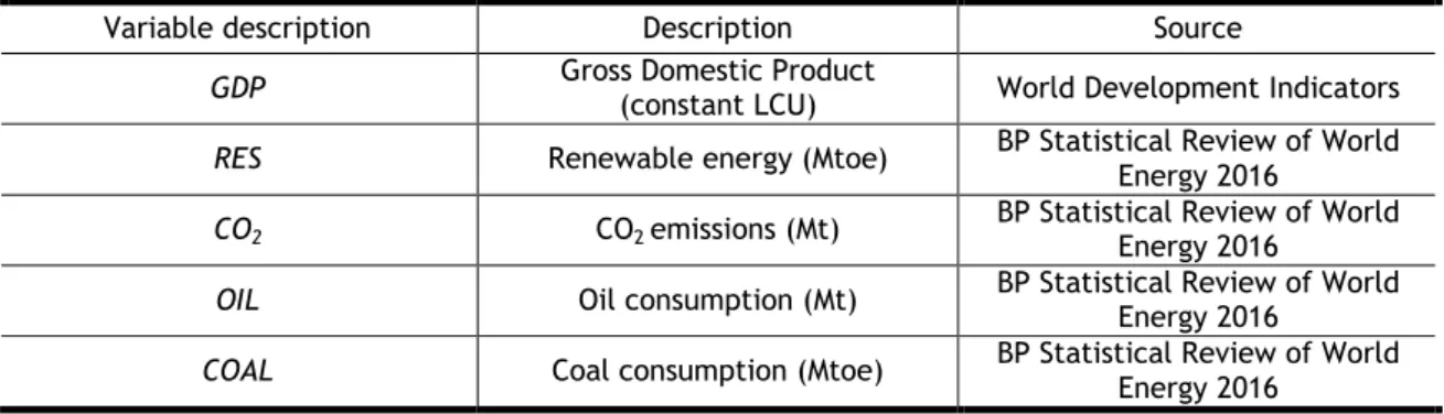
The time period used was from 1965 to 2015, totalling 51 years. This period was chosen because of the data available. The following table (Table 2) describes the variables, their units of measurement and sources:
Table 2: Variables
Variable description Description Source
GDP Gross Domestic Product (constant LCU) World Development Indicators
RES Renewable energy (Mtoe) BP Statistical Review of World Energy 2016
CO2 CO2 emissions (Mt) BP Statistical Review of World Energy 2016
OIL Oil consumption (Mt) BP Statistical Review of World Energy 2016
COAL Coal consumption (Mtoe) BP Statistical Review of World Energy 2016 Notes: Mtoe – Millions of tonnes in oil equivalent; Mt - Million tonnes; Constant LCU –Local currency unit; L – Natural logarithm.
The variables COAL and OIL were transformed into percentages of primary energy consumption, and the variable CO2 was transformed into CO2 intensity to reduce the correlation between the variables. In order to obtain the growth rates of the respective variables by the differenced logarithms, all variables were transformed into their natural logarithms. This transformation also reduced the phenomenon of heteroskedasticity. The following table present the descriptive statistics:
Table 3: Descriptive statistics
Mean Max. Min. Std. Dev JB Obs.
LCOAL_P 3.7003 3.8835 3.5390 0.0831 2.4551 51
LCO2_INT 1.1490 1.1924 1.1020 0.0186 1.7052 51
LRES 1.2779 2.0935 0.5460 0.3442 0.6421 51
LGDP 27.337 28.1135 26.456 0.4827 2.7379 51
LOIL_P 3.6834 3.9699 3.4726 0.1643 5.7805 51
Notes: Max. – Maximum; Min. – Minimum; Std. Dev. – Standard deviation; JB – Jarque-Bera; Obs – Observations.
8
After transforming the variables and interpreting the descriptive statistics, unit root tests were performed to determinate the integration order of the variables. The variables may be integrated of order zero or one, but cannot be integrated of order two. The results of the unit root tests are presented in next subsection.
3.2 Preliminary analysis
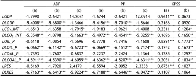
To determinate the integration order of the variables, the traditional unit root tests were performed, namely: ADF (Dickey and Fuller, 1981), PP (Phillips and Perron, 1988) and KPSS (Kwiatkowski et al., 1992). In both the ADF and PP tests, the null hypothesis is that the variable is non-stationary, i.e., there is a unit root. The opposite happens in the KPSS test, in which the null hypothesis is that the variable is stationary. The following table shows the results of the tests.
Table 4: Results of unit root tests
ADF PP KPSS
(a) (b) (c) (a) (b) (c) (a) (b)
LGDP -1.7990 -2.6421 14.2031 -1.6744 -2.6421 12.0914 0.9611*** 0.0673 DLGDP -5.4008*** -5.6800*** -1.3466 -5.4156*** -5.7010*** -1.5646 0.2166 0.0920 LCO2_INT -1.6513 -1.6358 -1.7915* -1.9183 -1.9621 -1.4008 0.2311 0.1204* DLCO2_INT -5.3548*** -1.0798 -5.1663*** -5.4972*** -5.4541*** -5.3255*** 0.1696 0.1650** LOIL_P -0.6118 -1.0854 -1.5696 -0.7778 -1.7416 -1.1608 0.8291*** 0.1773** DLOIL_P -6.0662*** -6.1142*** -5.6723*** -6.0669*** -6.1512*** -5.7174*** 0.1742 0.1673** LCOAL_P -1.7393 -1.7607 -0.6837 -2.2237 -2.2424 -1.1364 0.1285 0.1252* DLCOAL_P -4.5911*** -4.5390*** -4.6059*** -4.6362*** -4.5207*** -4.6311*** 0.2031 0.1834** LRES -0.5169 -1.7920 2.4179 -0.5594 -2.0052 2.3338 0.8751*** 0.1027 DLRES -6.7163*** -6.6413*** -5.9224*** -6.7188*** -6.6446*** -6.0472*** 0.1107 0.1064 Notes: (a) - Intercept; (b) - Trend and Intercept; (c) – None; *** - 1%; ** - 5%; * - 10%; D – first differences; ADF - Augmented Dickey-Fuller; PP - Phillips-Perron; KPSS - Kwiatkowski–Phillips–Schmidt– Shin.
From observing Table 4, it is possible to conclude, that all variable are stationary in first differences, and they are I(1). Nevertheless, structural breaks were observed, which can limit the traditional unit root test. Therefore, the unit root test with structural breaks Zivot and Andrews, (1992) (ZA), was performed, Table 5.
9
Given the existence of structural breaks, the ZA unit root test with structural breaks provides information on the specific period in which they occur. This information is useful for determining whether to apply dummies when the models are being estimated. The characteristics of the data under consideration did not compromise the use of the ARDL approach chosen.
The Variance Inflation Factor (VIF) test was performed and suggested the presence of multicollinearity between LGDP and LOIL_P. Consequently, models were estimated with both variables, and without LOIL_P, to confirm if the existence of multicollinearity would change the results. Comparing the results of these estimates, it was possible to conclude that there was no change in the signs, so that multicollinearity would not be a problem for estimating the model with all the variables.
3.2 Method: Autoregressive Distributed Lag
In order to analyse the short- and long-run relationship between all variables used, the approach chosen was the ARDL model, developed by Pesaran et al., (2001). Bearing in mind the characteristics of the data, a period of 51 years was studied. During such a lengthy period, it is likely that several statistically significant events will have occurred and, as such, they should be identified by testing. The ARDL model allows dummies to be applied without affecting the results, allows the treatment of endogeneity, the analysis of direct and indirect effects in the elasticities, and provides unbiased long-run estimation (Ahmad and Du, 2017). This model also allows for the separation of short- and long-run effects, which is important for determining if variables have different effects in the short- and long-run, and consequently makes it possible to confirm implicit causalities between all variables, through the existence of long-run relationships of cointegration.
The following equation represents the general Unrestricted Error Correction Model (UECM) equivalent to the ARDL bounds test used in the five ARDL models estimated:
𝐷𝒀𝒕= 𝛼0+ 𝛼1𝑇𝑅𝐸𝑁𝐷 + 𝛼2𝐷𝒁𝒕+ 𝛼3∑𝑘𝑝=1𝒀𝒕−𝒑+ 𝛼4∑𝑘𝑝=1𝒁𝒕−𝒑+ 𝜀𝑡, (1) Table 5: Results Zivot and Andrews unit root tests (4 lags)
(a) Break point (b) Break point (c) Break point
LGDP -4.5734 1998 -3.9416 1993 -4.5681 1998
LCO2_INT -4.0289 2007 -5.0246*** 2006 -4.8569* 2004
LOIL_P -3.8606 1980 -5.2880*** 1990 -4.9039* 1991
LCOAL_P -3.7892 2007 -4.1738* 2003 -4.0073 2002
LRES -3.6329 1987 -4.6758** 2008 -4.7460 2008
10
where, D denotes the first differences of variables, 𝑌𝑡 represents all the logarithm dependent
variables, 𝑍𝑡 represent all the logarithm independent variables, 𝛼2𝑖 is the short-run
coefficients, 𝛼3𝑖 is the Error Correction Model (ECM), 𝛼4𝑖 is the long-run coefficients and 𝜀𝑡 is
a white-noise error term.
The reverse models were estimated analysing the optimal number of lags necessary. The significance of the parameters was observed, and the residues were examined to ensure the estimations were as parsimonious as possible. After estimation of the models, diagnostics tests were performed, namely: the Jarque-Bera normality test (including Skewness, Kurtosis and Jarque-Bera), the Breusch-Godfrey serial correlation LM test, the ARCH test for heteroskedasticity, the Ramsey RESET test in order to model specification, and the stability tests of CUSUM and CUSUM squares.
The ARDL bounds test (Pesaran et al., 2001) was calculated with the null hypothesis of non-existence of cointegration, which means there is no long-run relationship. In addition, the short-run semi-elasticities and long-run elasticities were calculated. Semi-elasticities result directly from the coefficients of the model variables in the short run, and the elasticities were calculated as follows: The coefficient number of the variable in question, for instance c(6), was divided by the coefficient number of the ECM, for instance c(5), and the ratio multiplied by -1, using the following equation: [𝑐(𝑣𝑎𝑟) ⁄ 𝑐(𝐸𝐶𝑀)]) ∗ (−1) = 0.
11
4. Results
In this section the results of estimating the ARDL models, and the diagnostic tests to which they were submitted, are presented. The ARDL bounds test results are then shown, along with the calculations of the semi-elasticities and elasticities.
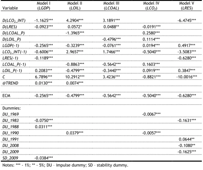
Considering the objective of studying the relationships between all the variables, five models were estimated. The results of all the models are presented on the following table:
Table 6: ARDL estimation
Variable Model I (LGDP) Model II (LOIL) Model III (LCOAL) Model IV (LCO2) Model V (LRES) D(LCO2_INT) -1.1625*** 4.2904*** 3.1891*** -6.4745*** D(LRES) -0.0923*** 0.0572* 0.0488** -0.0191*** D(LCOAL_P) -1.3965*** 0.2580*** D(LOIL_P) -0.4796*** 0.1114*** LGDP(-1) -0.2565*** -0.3239*** -0.0761*** 0.0194*** 0.4917*** LCO2_INT(-1) -0.6006*** 2.9657*** 1.7466*** -0.5040*** -3.5083*** LRES(-1) -0.1189*** -0.6280*** LCOAL_P(-1) -0.8863*** -0.5642*** 0.1603*** LOIL_P(-1) 0.2083*** -0.4799*** -0.3440*** 0.0919*** 0.3847*** C 6.7896*** 10.2912*** 3.4236*** -0.8821*** -10.0016*** @TREND 0.0130*** 0.0074*** ECM -0.2565*** -0.4799*** -0.5642*** -0.5040*** -0.6280*** Dummies: DU_1969 -0.0067*** DU_1983 -0.0750*** -0.1631*** DU_1988 0.0311*** DU_1990 0.0379*** -0.0057*** DU_1991 0.0644** DU_2008 -0.1080** DU_2009 -0.1625*** SD_2009 -0.0384***
Notes: *** - 1%; ** - 5%; DU – impulse dummy; SD – stability dummy.
After the estimation, diagnostic tests were performed that confirmed the normal behaviour of the residuals, the rejection of serial correlation of first and second order, the homoskedasticity of the residues, the correct specification of the model, and the stability of the parameters during the period studied, as shown in Table 7.
12 Table 7: Diagnostic tests
ARS 0.6728 0.7872 0.9174 0.9204 0.7376 SER 0.0093 0.0113 0.0078 0.0018 0.0393 JB 1.2252 1.7295 4.1417 1.8881 1.0289 LM (1) 0.3084 (1) 0.3058 (1) 0.7315 (1) 0.1192 (1) 0.0056 (2) 1.3784 (2) 0.1904 (2) 1.1946 (2) 1.0445 (2) 0.6345 ARCH (1) 0.1580 (1) 0.4147 (1) 0.2787 (1) 1.4230 (1) 0.1374 (2) 0.2356 (2) 1.2351 (2) 0.5500 (2)0.8721 (2) 0.1360 RESET 0.0135 0.1310 1.9517 1.2387 2.8027
CUSUM and CUSUM of squares test
Model I (LGDP):
Model II (LOIL):
13 Model IV (LCO2):
Model V (LRES):
Notes: the results are based on F - statistic; () – lag order; ARS – Adjusted R-squared; SER – S.E. of regression; JB – Jarque-Bera test; LM – teste Breusch-Godfrey; ARCH – teste ARCH; RESET – teste Ramsey RESET.
From Table 6 it is possible conclude that the ECM of all models is within an interval between -1 and 0 and revels a good adjustment velocity.
Regarding the dummies applied in model I-LGDP, the dummy in 1983 can be explained by the liberalisation and deregulation of the economy, 1988 was the year when Australia’s economic growth fell below the average rate of the other advanced economies, and 2009 represented the worst year of economic growth in all the years of consecutive growth. In model II-LOIL, the unit root test with structural breaks reveals a break point in 1990. With respect to model IV-LCO2, on the one hand, the consumption of natural gas increased in 1969, and caused an exponential increase in CO2 emissions, on the other hand, a high level of CO2 emissions occurred in 1990, and this year became the base year of the Kyoto protocol. The last model V-LRES, has dummies in 1983, which was the year that Australia had less production of renewable energy, 1990 was the year that the Renewable Energy Target encouraged the growth of wind capacity, a break point was detected in the ZA test in 2008, and 2009 was when the Australian government signed a contract to accelerate energy efficiency.
14
Considering all the results obtained from the five models, certain results can be highlighted. On one hand, the negative impact of LCO2_INT on LGDP, as well as of LRES on LGDP and LGDP
on LOIL_P and LCOAL_P. On the other hand, the positive impact of LCO2_INT on LCOAL_P and
LOIL_P, as well as of LGDP on LCO2_INT and LRES, and LOIL_P on LRES. Also, of note is the
absence of any impact by LRES on LCO2_INT in the long-run.
Table 8: ARDL Bounds test Value
F-Statistic k Bottom Top
Model I (LGDP) 9.7786*** 3 5.17 6.36
Model II (LOIL) 8.1340*** 3 5.17 6.36
Model III (LCOAL) 8.0068*** 3 4.29 5.61
Model IV (LCO2) 10.453*** 3 4.29 5.61
Model V (LRES) 11.4589*** 3 4.29 5.61
Notes: *** - 1%; Critical values of Pesaran et al., 2001; K – Number of long-run variables.
The ARDL bounds test was performed by an analysis of the F-statistic in the Wald test and the aforementioned null hypothesis was rejected. This meant that there was a long-run relationship between the variables (cointegration).
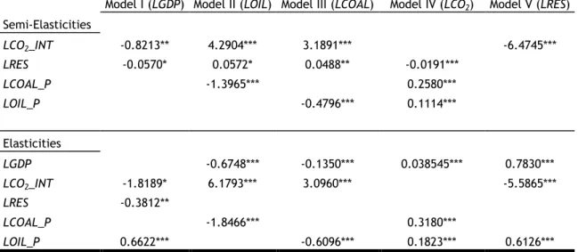
As previously mentioned, the direct and indirect effects on elasticities, semi-elasticities and elasticities were calculated.
Table 9: Semi-Elasticities and Elasticities
Model I (LGDP) Model II (LOIL) Model III (LCOAL) Model IV (LCO2) Model V (LRES) Semi-Elasticities LCO2_INT -0.8213** 4.2904*** 3.1891*** -6.4745*** LRES -0.0570* 0.0572* 0.0488** -0.0191*** LCOAL_P -1.3965*** 0.2580*** LOIL_P -0.4796*** 0.1114*** Elasticities LGDP -0.6748*** -0.1350*** 0.038545*** 0.7830*** LCO2_INT -1.8189* 6.1793*** 3.0960*** -5.5865*** LRES -0.3812** LCOAL_P -1.8466*** 0.3180*** LOIL_P 0.6622*** -0.6096*** 0.1823*** 0.6126*** Notes: *** - 1%; ** - 5%; * - 10%.
From the results in Table 9, it can be concluded that, in model I-LGDP, in the long-run, an increase of 1% in LCO2_INT, and LRES causes decreases in LGDP of 1.82% and 0.38%
respectively, and an increase of 1% in LOIL_P causes an increase of 0.66% in LGDP. In the short-run, in percentage points, LCO2_INT and LRES decrease LGDP by 0.82 and 0.06
respectively. Among the other results, the model IV-LCO2 should be highlighted, in which increases of 1% in LGDP, LCOAL_P and LOIL_P create increases in LCO2_INT of 0.04%, 0.32%
15
and 0.18% respectively. In the short-run, variations in LRES, LCOAL_P and LOIL_P lead respectively to a decrease of 0.02 and increases of 0.26 and 0.11 in LCO2_INT, in percentage
16
5. Discussion
On the whole, Australia is a country with a strong economic path, surpassing the Netherlands, in 2017, as the country with longest consecutive number of years without a recession. This makes Australia an attractive subject for investigation. This study makes a deeper analysis of the relationship, in both the short- and long-run, between GDP, CO2 intensity, fossil fuels (coal and oil) consumption, and RES consumption in Australia. In brief, the following diagrams synthesize the implicit causalities founded.
Figure 1: Short- and long-run causalities
Source: Own elaboration
Notes: long-run unidirectional relationship →; long-run bidirectional relationship ↔; short-run
unidirectional relationship ; short-run bidirectional relationship
Our findings prove that LCO2_INT and LRES have caused a slowdown in economic growth,
although insufficient to interrupt strong economic activity and continuous growth. This decrease can be explained by the huge investment needed to expand RES capacity and by restrictive energy consumption policies that reduce CO2 intensity, and consequently, LGDP. This effect shows that it is possible for a country to address environmental preoccupations, not just emissions reduction but also mix diversification, while continuing to experience economic growth. Regarding the effects of LGDP on LRES and on LCO2_INT, on the one hand,
higher GDP leads to higher RES consumption (Saidi and Ben Mbarek, 2016) because, with increased GDP, the country invests more in renewable energy. On the other hand, increasing GDP implies more energy consumption, and considering that the renewable technology is limited, the energy consumed are the fossil fuels which increase the CO2 emissions (Bilgili et al., 2016). Despite its growing GDP, Australia has a high level of CO2 intensity, and LRES only decreases it in the short-run. LRES causes a decrease in CO2 intensity by avoiding the burning of fossil fuels, given that primary energy consumption remains constant. In the long-run, RES has no impact, because the renewable technology used has limited and insignificant potential growth.
With regard to fossil fuels, Australia has extensive reserves. However, based on empirical evidence, this paper confirms that there is a negative relationship between LGDP and
RES GDP
CO2
COAL
17
LCOAL_P and LOIL_P. This effect confirms that Australia intends to diversify its energy mix
promoting substitution. With growing LGDP, primary energy consumption increases, and the mix of primary energy consumption increases LRES. In view of this, the country is investing in clean energy and measures to promote energy efficiency to achieve environmental targets. Therefore, with growing LGDP, the LOIL_P and LCOAL_P are reduced. In addition to the effect of fossil fuels on the economy, they are also associated with environmental degradation. Fossil fuels are considered the main cause of the high CO2 emissions. The empirical results show that fossil fuels consumption increase LCO2_INT (Ito, 2017). If primary energy
consumption remains constant and the consumption of fossil fuels increases in the mix, CO2 emissions increase.
Australia has defined environmental targets to reduce CO2 emissions by between 26% and 28% by the year 2030, based on 2005 values, in accordance with the Paris agreement. In view of the results obtained, one way to be successful would be to apply policies to reduce coal consumption. A variation of 1% in LCOAL_P causes an increase of the 0.32% in LCO2_INT, and
this variable has the greatest impact in both the short- and long-run. RES can also be used to achieve environmental targets, and to do so, it is necessary to understand which variables influence it. LRES is encouraged by LOIL_P (Saidi and Ben Mbarek, 2016). This effect could be explained as an effect of a growing economy, in other words, the Australian economy. On one hand, the economy continues to be dependent on oil, and this dependency helps economic growth, and on the other hand, the economy invests in renewable energy. This also explains the positive effect of LOIL_P on LGDP. In addition, Australia should invest in energy efficiency measures, specifically tailored to certain economic sectors. It was confirmed that Australia needs to slow down its economic growth to achieve better environmental quality, and reduce CO2 emissions.
18
6. Conclusion
This paper analyses the relationship between economic activity through LGDP, energy consumption through LCOAL_P, LOIL_P and LRES, and environmental degradation through
LCO2_INT, and focuses on Australia. With this objective, all relationships were studied, and
this meant that five models were estimated with all variables as dependent variables. The ARDL methodology was employed to study the dynamics of adjustment for a period from 1965 to 2015. This approach was selected due to its ability to apply dummies without affecting the results, considering the 51 years studied during the course of which events may have occurred which must be controlled. The separation of short- and long-run effects is also important to understand if the variables behave in the same way in the short- and long-run, and if it is possible to conclude whether there are implicit causalities between all the variable, through the existence of long-run relationships of cointegration.
There is no consensus in the literature on the energy-growth nexus about the causalities between economic growth and energy consumption. This could be explained by the fact that different variables, periods, countries and methods were used. Empirical evidence for Australia remains scarce, which leads to the main aim of this research. In fact, it is important to examine the energy-growth nexus question in a country that has had no recession for several consecutive years, and increasingly experienced economic growth. The results of this study confirm the feedback hypothesis between economic growth and both oil and RES consumption. Furthermore, the conservation hypothesis is supported by economic growth and coal consumption. Concerning the relationship between economic growth and CO2 intensity, the results are entirely different. Economic growth increases CO2 intensity, while CO2 intensity has a negative impact on GDP. In other words, in Australia, there is a trade-off between economic development and environmental quality. Overall, the finding of implicit causalities in the ARDL models revealed a strong consistency.
To achieve its environmental goals, Australia should change its energy mix, in other words, change the relative consumption of the different energy types to reduce CO2 emissions, without changing the amount of primary energy consumed. Another alternatives would be: applying policies to restrict fossil fuels consumption, particularly coal; energy efficiency measures; and investing in RES technology, to increase RES consumption.
19
References
Acaravci, A. and Ozturk, I. (2010), “On the relationship between energy consumption, CO2 emissions and economic growth in Europe”, Energy, Elsevier Ltd, Vol. 35 No. 12, pp. 5412–5420.
Ahmad, N. and Du, L. (2017), “Effects of Energy Production and CO2 emissions on Economic Growth in Iran: ARDL Approach”, Energy, Elsevier Ltd, Vol. 123, pp. 521–537.
Alshehry, A.S. and Belloumi, M. (2015), “Energy consumption, carbon dioxide emissions and economic growth: The case of Saudi Arabia”, Renewable and Sustainable Energy Reviews, Elsevier, Vol. 41, pp. 237–247.
Ang, J.B. (2007), “CO2 emissions, energy consumption, and output in France”, Energy Policy, Vol. 35 No. 10, pp. 4772–4778.
Antonakakis, N., Chatziantoniou, I. and Filis, G. (2017), “Energy consumption, CO2 emissions, and economic growth: An ethical dilemma”, Renewable and Sustainable Energy Reviews, Elsevier, Vol. 68 No. November 2016, pp. 808–824.
Appiah, M.O. (2018), “Investigating the multivariate Granger causality between energy consumption, economic growth and CO 2 emissions in Ghana”, Energy Policy, Elsevier Ltd, Vol. 112 No. April 2017, pp. 198–208.
Arvin, M.B., Pradhan, R.P. and Norman, N.R. (2015), “Transportation intensity, urbanization, economic growth, and CO<inf>2</inf> emissions in the G-20 countries”, Utilities Policy, Elsevier Ltd, Vol. 35, pp. 50–66.
Balsalobre-Lorente, D., Shahbaz, M., Roubaud, D. and Farhani, S. (2018), “How economic growth, renewable electricity and natural resources contribute to CO2emissions?”, Energy Policy, Elsevier Ltd, Vol. 113 No. November 2017, pp. 356–367.
Bekhet, H.A., Matar, A. and Yasmin, T. (2017), “CO2 emissions, energy consumption, economic growth, and financial development in GCC countries: Dynamic simultaneous equation models”, Renewable and Sustainable Energy Reviews, Vol. 70 No. November 2016, pp. 117–132.
Bilgili, F., Koçak, E. and Bulut, Ú. (2016), “The dynamic impact of renewable energy consumption on CO2 emissions: A revisited Environmental Kuznets Curve approach”, Renewable and Sustainable Energy Reviews, Elsevier, Vol. 54, pp. 838–845.
20
Algeria”, Energy Policy, Elsevier, Vol. 96, pp. 93–104.
Cai, Y., Sam, C.Y. and Chang, T. (2018), “Nexus between clean energy consumption,
economic growth and CO2 emissions”, Journal of Cleaner Production, Elsevier Ltd, Vol. 182, pp. 1001–1011.
Chen, P.Y., Chen, S.T. and Chen, C.C. (2012), “Energy consumption and economic growth-New evidence from meta analysis”, Energy Policy, Elsevier, Vol. 44, pp. 245–255. Destek, M.A. and Aslan, A. (2017), “Renewable and non-renewable energy consumption and
economic growth in emerging economies: Evidence from bootstrap panel causality”, Renewable Energy, Elsevier Ltd, Vol. 111, pp. 757–763.
Dickey, D. and Fuller, W. (1981), “Likelihood ratio statistics for autoregressive time series with a unit root”, Econometrica, Vol. 49 No. 4, pp. 1057–1072.
Eggoh, J.C., Bangake, C. and Rault, C. (2011), “Energy consumption and economic growth revisited in African countries”, Energy Policy, Elsevier, Vol. 39 No. 11, pp. 7408–7421. Fuinhas, J.A. and Marques, A.C. (2012), “Energy consumption and economic growth nexus in
Portugal, Italy, Greece, Spain and Turkey: An ARDL bounds test approach (1965-2009)”, Energy Economics, Elsevier B.V., Vol. 34 No. 2, pp. 511–517.
Gozgor, G., Lau, C.K.M. and Lu, Z. (2018), “Energy consumption and economic growth: New evidence from the OECD countries”, Energy, Elsevier Ltd, Vol. 153, pp. 27–34.
Grossman, G.M. and Krueger, A.B. (1991), “Environmental Impacts of a North American Free Trade Agreement”, National Bureau of Economic Research Working Paper Series, Vol. No. 3914 No. 3914, pp. 1–57.
IEA. (2012), Energy Policies of IEA Countries - Australia 2012 Review, available at:https://doi.org/10.1787/9789264170841-en.
International Energy Agency (IEA). (2018), “Energy Policies of IEA Countries: Australia 2018 Review”, p. 244.
Ito, K. (2017), “CO2 emissions, renewable and non-renewable energy consumption, and economic growth: evidence from panel data for developing countries”, International Economics, Elsevier, No. xxxx, pp. 1–6.
Jammazi, R. and Aloui, C. (2015), “On the interplay between energy consumption, economic growth and CO2 emission nexus in the GCC countries: A comparative analysis through
21
wavelet approaches”, Renewable and Sustainable Energy Reviews, Elsevier, Vol. 51, pp. 1737–1751.
Kais, S. and Sami, H. (2016), “An econometric study of the impact of economic growth and energy use on carbon emissions: Panel data evidence from fifty eight countries”, Renewable and Sustainable Energy Reviews, Elsevier, Vol. 59, pp. 1101–1110.
Kaya, Y. (1990), “Impact of Carbon Dioxide emission control on GNP growth: Interpretation of proposed scenarios”, Paper Presented to the IPCC Energy and Industry Subgroup,
Response Strategies Working Group.
Kraft, J. and Kraft, A. (1978), “On the relationship between energy and GNP”, Journal of Energy and Development, Vol. 3, pp. 401–403.
Kuznets, S. (1955), “Economic growth and income inequality”, The American Economic Review, Vol. 45 No. 1, pp. 1–28.
Kwiatkowski, D., Phillips, P.C.B., Schmidt, P. and Shin, Y. (1992), “Testing the null hypothesis of stationarity against the alternative of a unit root”, Journal of Econometrics, Vol. 54 No. 1–3, pp. 159–178.
Lim, G.C., Chua, C.L., Claus, E. and Nguyen, V.H. (2012), “Review of the Australian Economy 2011-12: A Case of Déjà Vu”, Australian Economic Review, Vol. 45 No. 1, pp. 1–13. Magazzino, C. (2018), “GDP, energy consumption and financial development in Italy”,
International Journal of Energy Sector Management, Vol. 12 No. 1, pp. 28–43. Mehrara, M. (2007), “Energy consumption and economic growth: The case of oil exporting
countries”, Energy Policy, Vol. 35 No. 5, pp. 2939–2945.
Menegaki, A.N. (2011), “Growth and renewable energy in Europe: A random effect model with evidence for neutrality hypothesis”, Energy Economics, Elsevier B.V., Vol. 33 No. 2, pp. 257–263.
Menyah, K. and Wolde-Rufael, Y. (2010), “Energy consumption, pollutant emissions and economic growth in South Africa”, Energy Economics, Elsevier B.V., Vol. 32 No. 6, pp. 1374–1382.
Mirza, F.M. and Kanwal, A. (2017), “Energy consumption, carbon emissions and economic growth in Pakistan: Dynamic causality analysis”, Renewable and Sustainable Energy Reviews, Elsevier Ltd, Vol. 72 No. October 2016, pp. 1233–1240.
22
Narayan, P.K. and Narayan, S. (2010), “Carbon dioxide emissions and economic growth: Panel data evidence from developing countries”, Energy Policy, Elsevier, Vol. 38 No. 1, pp. 661–666.
Panayotou, T. (1993), “Empirical tests and policy analysis of environmental degradation at different stages of economic development”, Technology Environment and Employment Geneva International Labour Office.
Pesaran, M.H., Shin, Y. and Smith, R.J. (2001), “Bounds testing approaches to the analysis of long run relationships”, Journal of Applied Econometric, Vol. 16, pp. 289–326.
Phillips, P.C.B. and Perron, P. (1988), “Testing for a unit root in time series regression”, Biometrika, Vol. 75 No. 2, pp. 335–346.
Rank, W., Rank, R. and Status, E.F. (2017), “81.0 ( ▲”, No. September 2015, pp. 112–113. Saidi, K. and Hammami, S. (2015), “The impact of CO2 emissions and economic growth on
energy consumption in 58 countries”, Energy Reports, Elsevier Ltd, Vol. 1, pp. 62–70. Saidi, K. and Ben Mbarek, M. (2016), “Nuclear energy, renewable energy, CO2 emissions, and
economic growth for nine developed countries: Evidence from panel Granger causality tests”, Progress in Nuclear Energy, Elsevier Ltd, Vol. 88, pp. 364–374.
Shahbaz, M., Zakaria, M., Shahzad, S.J.H. and Mahalik, M.K. (2018), “The energy consumption and economic growth nexus in top ten energy-consuming countries: Fresh evidence from using the quantile-on-quantile approach”, Energy Economics, Elsevier B.V., Vol. 71, pp. 282–301.
Soytas, U., Sari, R. and Ewing, B.T. (2007), “Energy consumption, income, and carbon emissions in the United States”, Ecological Economics, Vol. 62 No. 3–4, pp. 482–489. Streimikiene, D. and Kasperowicz, R. (2016), “Review of economic growth and energy
consumption: A panel cointegration analysis for EU countries”, Renewable and Sustainable Energy Reviews, Vol. 59, pp. 1545–1549.
Tang, C.F. and Abosedra, S. (2014), “The impacts of tourism, energy consumption and political instability on economic growth in the MENA countries”, Energy Policy, Elsevier, Vol. 68, pp. 458–464.
Tiba, S. and Omri, A. (2017), “Literature survey on the relationships between energy,
environment and economic growth”, Renewable and Sustainable Energy Reviews, Vol. 69 No. October 2016, pp. 1129–1146.
23
Tugcu, C.T. and Topcu, M. (2018), “Total, renewable and non-renewable energy consumption and economic growth: Revisiting the issue with an asymmetric point of view”, Energy, Elsevier Ltd, Vol. 152, pp. 64–74.
Vidyarthi, H. (2015), “Energy consumption and growth in South Asia: evidence from a panel error correction model”, International Journal of Energy Sector Management, Vol. 9 No. 3, pp. 295–310.
Wang, S., Li, G. and Fang, C. (2018), “Urbanization, economic growth, energy consumption, and CO2emissions: Empirical evidence from countries with different income levels”, Renewable and Sustainable Energy Reviews, Elsevier Ltd, Vol. 81 No. July 2017, pp. 2144–2159.
Wang, S., Zhou, C., Li, G. and Feng, K. (2016), “CO2, economic growth, and energy consumption in China’s provinces: Investigating the spatiotemporal and econometric characteristics of China’s CO2 emissions”, Ecological Indicators, Elsevier Ltd, Vol. 69, pp. 184–195.
Zivot, E. and Andrews, D.W.K. (1992), “Further Evidence on the Great Crash, the Oil Price Shock, and the Unit Root Hypothesis”, Journal of Business & Economic Statistics, Vol. 10 No. 3, pp. 251–270.