Decision Trees for the Prediction of Outcome of Soccer Games - Historical
Data Analysis
Árvores de decisão para a previsão de resultados de Jogos de Futebol - Análise
de Dados Históricos
DOI:10.34117/bjdv6n1-339
Recebimento dos originais: 30/11/2019 Aceitação para publicação: 30/01/2020
Ercilia de Stefano
Doutora em Engenharia de Transportes - UFRJ Professora Adjunta - UFF Petrópolis Rua Domingos Silvério, 01 - Petrópolis - RJ
E-mail: ercilia.stefano@gmail.com
Leonardo de Oliveira Farroco
Especialista em Gestão da Tecnologia da Informação Analista de Sistemas Sênior
Rua Antônio da Silva Ligeiro - Petrópolis - RJ
Gilson Brito Alves Lima
Doutor em Engenharia de Produção, UFRJ Professor Titular UFF - Niterói
R. Passo da Pátria, 156 - Boa Viagem - Boa Viagem, Niterói - RJ, 24210-240
Annibal Parracho Sant'Anna
Doutor em Estatística pela Universidade da California - Berkeley Professor titular da Universidade Federal Fluminense
R. Passo da Pátria, 156 - Boa Viagem - Boa Viagem, Niterói - RJ, 24210-240
Luiz Octávio Gavião
Doutor em Engenharia de Produção na UFF Professor Adjunto na Escola Superior de Guerra (ESG)
Fortaleza de São João - Av. João Luiz Alves, s/nº - Urca – Rio de Janeiro-RJ - CEP: 22291-090
Vitor Ayres Principe
Doutorando em Gestão da Informação na Management School da Universidade Nova de Lisboa Professor na Universidade Estácio de Sá e Faculdade Enau
Endereço comercial: Estácio: R. Gen. Alfredo Bruno Gomes Martins, s/n - Lote 19 - Braga, Cabo Frio – RJ
ABCTRACT
This paper presents the design and results of the submission from the researchers from Universidade Federal Fluminense (UFF) to the Machine Learning Soccer Prediction Challenge, organized by the Springer Machine Learning Journal. The steps of parsing of data, building of the model and choice of a Decision Tree for predicting the results from soccer matches are explained and discussed. This study also analyses the variation of the win percentage of home teams in different countries. Some possibilities to explain these variations, such as country size and training infrastructure are raised. The intention is to provide researchers in the field with insights for additional data that may help the prediction of games in regions with diverse patterns.
Keywords: Decision Tree, Soccer, Prediction, Machine Learning RESUMO
Este artigo apresenta o design e os resultados da submissão dos pesquisadores da Universidade Federal Fluminense (UFF) ao Desafio de Previsão de Futebol de Aprendizado de Máquina, organizado pelo Springer Machine Learning Journal. As etapas de análise de dados, construção do modelo e escolha de uma Árvore de Decisão para prever os resultados de partidas de futebol são explicadas e discutidas.
Este estudo também analisa a variação da porcentagem de vitórias de equipes em casa em diferentes países. Algumas possibilidades para explicar essas variações, como tamanho do país e infraestrutura de treinamento, são levantadas. A intenção é fornecer aos pesquisadores do campo informações para dados adicionais que possam ajudar na previsão de jogos em regiões com diversos padrões.
Palavras-chave: Árvore de Decisão, Futebol, Previsão, Aprendizado de Máquina
1 INTRODUCTION
The sports prediction area is a fertile field to explore and expand the capabilities of machines employed to solve problems (Sheppard, 1998). With more than 265 million players worldwide, both male and female, soccer is the sport with more practitioners – achieving four percent of the world population (FIFA, 2007). The sports offer many challenges and opportunities to explore one’s skills and find strategies for personal advance (Sheppard, 1998). There is an interaction between the highly stochastic nature of the game and the highly structured set of rules and strategies that can be employed (Min, Kim, Choe, Eom, & McKay, 2008).
Performance in soccer has been described as an intersection in individual and collective levels (Bradley et al., 2011). The results of a soccer game can provide objective measures about the performance of each player and his or her team. Interactions inside a team can be considered as a cooperation based in a strategic plan, situational variables and restrictions in the general game context (Besters et al., 2016). Even controlling these metrics, soccer still has expected and unexpected facts that influence the result from a match (Aslan, 2007).
This way, a complete comprehension of the types of information employed in the process is crucial. Some information is easily identified, but, when the set of needed information is considered, identifying less obvious information related to the decision process should be presented in a cohesive way and in the appropriated context (Alamar, 2013).
The present study intends to raise considerations on sets of variables that may provide this type of information and models that show relations between them. Information on previous performances are considered and the relations between them are assessed employing machine learning to evaluate the models.
This work was ranked #13 in the Machine Learning Journal Prediction Challenge. This work provides some lessons learned on how to improve score prediction. The submitted approach had an accuracy of 0.3592233 and a Ranked Probability Score of 0.4514563.
2 RELATED WORK
There are many works published about the prediction of soccer games and other sports. Current trends in soccer analysis show the usage of probabilistic models to simulate the matches’ actions and results (Brooks, Kerr, & Guttag, 2016). A usual approach is to model the result distribution by bivariate Poisson distributions. The works of Maher (1982) and Karlis and Ntzoufras (2003), introduced new ideas: to use a dependency parameter to improve the prediction of the number of draws. Dixon and Coles (1997) used a similar approach and developed a model that was capable to generate probabilities of results. Rue and Sabesen (2000) added the supposition that the parameters of attack and defense are temporal variables and used Bayesian methods to update their estimates, using Monte Carlo simulations to create inferences. Later, Crowder et al., (2012) developed a less expensive computational method to update the parameter estimates. Koopman and Lit (2015) highlighted the importance of transforming these models into dynamic models, as the forces of attack and defense of a team vary with time.
Another key reference material is the work of Rotshtein et al. (2005), where fuzzy logic and neural tuning allow the prediction of the outcome of games. Other studies with Operational Research approaches have been reached interesting results with probabilistic models. In Gaviao et. al. (2017), the Composition of Probabilistic Preferences (CPP), developed by Sant’Anna and Sant’Anna (2001), was adapted with the Gini Index to sort soccer players by regularity.
Other analyses deal with the prediction of results of events (for example, the success of match objectives), matches and competitions. The players’ performance is a key parameter to add precision to predictions. The prediction of player performance is a relevant topic with additional applications in the predictions related to technical performance (scouting) and to physical aptitude (Arndt and Brefeld, 2016). Reep and Benjamin (1968) developed models to success taxes of different pass sequences, being limited to the lack of access to data about the location of the passes. Recently, Constantinou (2012) and Collet (2013), predicted the results of games using ball passes scores in different teams and other historical statistics to develop probabilistic models.
Buraimo (2010) studied the effect of arbiters’ decisions about the matches’ results, in an attempt to determine the possible course introduced with the attribution of sanctions (red or yellow) in the English Premier League and German Bundesliga.
Another line of research approached the analysis about individual players, focusing in this capacity of scoring goals, where McHale and Szczepanski 92014) proposed two models with mixed results, separating the scoring process in the generation or shots and the conversion of shots to goals. The authors validated their models with data from two seasons from the English Premier League.
Finally, it is worth to point the contribution of Dijkhuizen (2012), which attempted to show the relation between the sports results and the economic performance in a given region. The MetrIA software (de Stefano et al., 2016) was used to carry out the literature searches of this paper.
3 GENERAL IDEAS
The main idea behind this approach is take into account that each league has its own characteristics. Playing styles, league organization and country size, which adds difficult adaptation to the away team, may have different importance for the teams in different leagues. Different leagues also display different strategies with respect, for instance, to teams playing more conservatively, an away team satisfied with a draw, not risking try to win.
As pointed by Stefani (1992), the advantage from the home team may come from different factors that have negative effects in the visiting team: physical fatigue caused by the travel; home team fans supporting their team and taunting/intimidating the visiting team and lack of familiarity with the environment (which the author calls a “tactical effect”).
The approach taken was then to pay first attention to the results of each league in a preliminary analysis of the data set. This leads to a first decision of separating performances at home and away. This decision came from the observation that the Home Win rate in the BRA1 league was of 50.8 percent.
In the analyzed dataset, the home team wins roughly 45% of the times:
Table 1 Overall home win, lose and draw percentages
Match Type Total Percentages Home Win 98443 45.41%
Home Lose 59540 27.47%
Home Draw 58760 27.11%
Total 216743 100%
The deviation from the historic average was small, but in individual leagues – where fewer games occurred – it was possible to identify larger deviations. T leagues with games in the prediction
set are among those with the greatest historical average of home wins. The predicted set of 206 games displayed less than 2 percent of deviation when compared with the overall data:
Table 2 Prediction set overall deviation from the historic data
Match Type Total Percentages Deviation Home Win 93 45.14% 0.27%
Home Lose 54 26.21% 0.89%
Home Draw 59 28.64% -1.17%
Total 206 100% 0
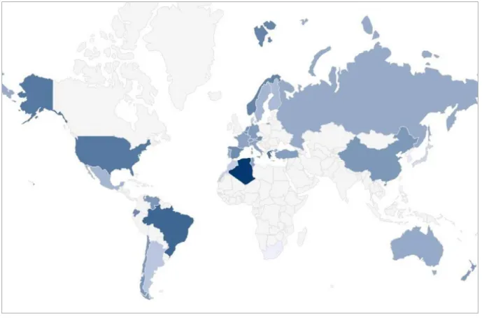
The map below displays the distribution of the home win chance percentage by country. Geography does not seem to heavily influence this rating. One point that might be considered is the variety of climates in a given region. The USA, Brazil, Chile, China and Spain (a country with regions with lower humidity) displayed higher win chance for the home teams. Argentina has a lower chance, but it may be argued that the population in that country is concentrated in the Buenos Aires region.
Fig. 1 Countries colored by their home win percentages (darker = higher home-win percentage, lighter = lower home-
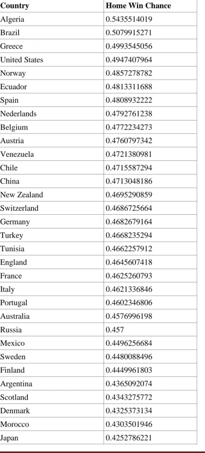
Figure 1 is a graphical representation of the data listed in the table below, wich includes the country name and its Home Win Chance (from 0 to 1). The list is sorted by higher win chance to lower.
Table 3 Countries listed by Home Win Chance
Country Home Win Chance
Algeria 0.5435514019 Brazil 0.5079915271 Greece 0.4993545056 United States 0.4947407964 Norway 0.4857278782 Ecuador 0.4813311688 Spain 0.4808932222 Nederlands 0.4792761238 Belgium 0.4772234273 Austria 0.4760797342 Venezuela 0.4721380981 Chile 0.4715587294 China 0.4713048186 New Zealand 0.4695290859 Switzerland 0.4686725664 Germany 0.4682679164 Turkey 0.4668235294 Tunisia 0.4662257912 England 0.4645607418 France 0.4625260793 Italy 0.4621336846 Portugal 0.4602346806 Australia 0.4576996198 Russia 0.457 Mexico 0.4496256684 Sweden 0.4480088496 Finland 0.4449961803 Argentina 0.4365092074 Scotland 0.4343275772 Denmark 0.4325373134 Morocco 0.4303501946 Japan 0.4252786221
Israel 0.4194690265
Korea 0.4087385483
South Africa 0.405520867
Other factors, related to the organization of the leagues, might help explain the variations between regions.
Leagues whose players participate in international competitions (such as the Euro Cup) during the whole season, helping the players to acclimate to different regions. Leagues with players that take part in other competitions, increasing their number of games per year) might also negatively impact visiting teams. Higher infrastructure of training fields and/or hotels might also help to explain the regional differences.
The differences point above is displayed in detail in table 3, as it shows the historical average of the leagues that performed in the prediction set games and the deviation from average of that matches to the previous average.
Table 4 Prediction set leagues deviation from the historic data
League Historic Average Prediction Set Deviation
HW HD HL HW HD HL HW HD HL AUT1 0,48 0,27 0,26 0,80 0,00 0,20 0,32 -0,27 -0,06 BEL1 0,48 0,28 0,25 1,00 0,00 0,00 0,52 -0,28 -0,25 CHE1 0,47 0,29 0,25 0,80 0,00 0,20 0,33 -0,29 -0,05 CHN1 0,47 0,23 0,29 0,50 0,13 0,38 0,03 -0,11 0,08 ECU1 0,48 0,25 0,27 0,50 0,17 0,33 0,02 -0,09 0,07 ENG1 0,46 0,28 0,26 0,30 0,40 0,30 -0,16 0,12 0,04 ENG2 0,44 0,28 0,28 0,08 0,67 0,25 -0,36 0,38 -0,03 FRA1 0,46 0,25 0,29 0,75 0,00 0,25 0,29 -0,25 -0,04 FRA2 0,45 0,23 0,32 0,50 0,20 0,30 0,05 -0,03 -0,02 GER1 0,47 0,29 0,24 0,56 0,33 0,11 0,09 0,05 -0,13 GER2 0,46 0,27 0,27 0,44 0,33 0,22 -0,01 0,06 -0,05 GRE1 0,50 0,25 0,25 0,25 0,13 0,63 -0,25 -0,13 0,38 HOL1 0,48 0,29 0,23 0,56 0,22 0,22 0,08 -0,06 -0,01 ISR1 0,42 0,30 0,28 0,43 0,43 0,14 0,01 0,12 -0,13 ITA1 0,46 0,26 0,28 0,40 0,20 0,40 -0,06 -0,06 0,12 JPN1 0,43 0,33 0,24 0,33 0,00 0,67 -0,09 -0,33 0,43 KOR1 0,41 0,30 0,29 0,67 0,33 0,00 0,26 0,03 -0,29 MEX1 0,45 0,27 0,28 0,56 0,33 0,11 0,11 0,07 -0,17 POR1 0,46 0,28 0,26 0,33 0,67 0,00 -0,13 0,39 -0,26 RUS1 0,46 0,27 0,27 0,00 0,75 0,25 -0,46 0,48 -0,02 SCO1 0,43 0,33 0,24 0,67 0,33 0,00 0,23 0,00 -0,24 SPA1 0,48 0,27 0,25 0,50 0,20 0,30 0,02 -0,07 0,05
TUN1 0,47 0,23 0,30 0,67 0,33 0,00 0,20 0,10 -0,30
USA1 0,49 0,23 0,27 0,60 0,10 0,30 0,11 -0,13 0,03
VEN1 0,47 0,25 0,28 0,33 0,22 0,44 -0,14 -0,02 0,16
ZAF1 0,41 0,29 0,31 0,50 0,38 0,13 0,09 0,09 -0,18
In order to take into account the current state, the number of points earned by the club in the League in the present season was considered. Another idea was to identify teams that are in a series of victories or losses, indicating that its performance is under or above average in that moment. On the other hand, to provide expand the view, the final position in the League standings in the previous season was also considered.
4 DATA PRE-PROCESSING AND FEATURE ENGINEERING
One key aspect of this study was to use just the data provided by the competition organizers. As statistics about individual players or coaches were not considered, the model used just the matches results to generate the others variables. Gambling ratings from external sources were not considerate. The main features above detached lead then to a series of variables describing the current status of the team.
The data was pre-processed in Node.js, as it is flexible enough to combine CSV files and export new ones to be shared with other researchers. The matches results provided by the challenge organizers was loaded by a script that performed the actions below:
Algotithm 1 Pseudocode for parsing a CSV with match data into the model Input:
games.csv: The training data provided by the challenge organizers, converted from xlsx to CSV
computeRow: a procedure (explained below)
Output:
model: A CSV file with additional variables 1: Read games.csv
2: Create Teams dictionary 3: for each row in games.csv do
4: row = computeRow(row, Teams dictionary)
5: Compute Previous Season Places 6: Write model
Algotithm 2 Pseudocode for computeRow procedure. Each row in the games.csv uses the
Input:
row: A line from the games.csv file
dict: A dictionary with the teams historical data
Output:
row: The same row provided in the input, but with additional variables 1: Read row and identify the home team and away team
2: for team in home team and away team
3: Read team name
4: if isANewTeam(team name)
5: add team to Teams dictionary
6: Read league name and season columns
7: Check if the season from the previous game is different from if current one 8: if the league has changed
9: reset season data (sets points in current season to 0)
10: if home team goals > away team goals then
11: for the home team
12: add a victory to the victory streak in the home team dictionary
13: set its losing streak to 0
14: set its tie streak to 0
15: set its wonLast as true
16: add 3 season points to the current season in the home team dictionary
17: for the away team
18: add a loss to the losing streak in the away team dictionary
19: set its winning streak to 0
20: set its tie streak to 0
21: set its wonLast as false
22: if the away team goals > home team goals then
23: for the away team
24: add a victory to the victory streak in the away team dictionary
25: set its losing streak to 0
26: set its tie streak to 0
27: set its wonLast as true
28: add 3 season points to the current season in the away team dictionary
29: for the home team
30: add a loss to the losing streak in the home team dictionary
31: set its winning streak to 0
32: set its tie streak to 0
33: set its wonLast as false
34: if home team goals == away team goals then
35: for both teams
36: add a tie to the tiestreak of the team
37: set its winning streak to 0
38: set its losing streak to 0
This shortened version of the algorithm allows to identify an important flaw in its inner working. In line 7 (“Check if the season from the previous game is different from if current one”) the computation concatenates the league name with the season to obtain a string. If this string is different from the previous one, than the algorithm considers that the season has changed. As games from the prediction set were marked as “run”, instead of the “16-17”, the algorithm assumed that a new season had begun. This had a negative impact in the model as it erased important variables, such as the difference of positions in the current season between the two teams. In order to avoid this error, the rows labeled with “run” should be renamed to “16-17” so that the pre-processing phase can place the correct values in each variable.
The pre-processing stage adds diverse variables to each row of data:
Winning, losing or tie streaks are identified with the variables “homeWinStreak”, “homeTieStreak”, “homeLoseStreak”, “awayWinStreak”, “awayTieStreak” and “awayLoseStreak” have the number of previous matches won/lost/draw by each team.
The winner of the last encounter between each team is also identified with the variables “HomeWonLastEncounter” and “lastEncounterWasTie”.
The position in which the two teams placed in the previous season is identified with the variables “homeLastSeasonPlace” and “awayLastSeasonPlace”. After the study was completed, the researchers identified that a single variable with the difference of positions between the two teams would suffice to display the ranking difference.
The position of both teams in the current teams is also registered with the variables “HomePoints”, “awayPoints” and “homeTeamRanksHigher”. As in the previous case, these variables could by replaced with a single one with the position difference. If the home team ranked higher the value would have a positive point different, or a negative point difference if the home team ranked lower. After the results were computed we identified that there were errors in building these variables that influenced the predicted score.
5 LEARNING ALGORITHM
This study employed Naive Bayes, Decision Tree and Random Decision Tree classifiers during the development. Overall, the Random Decision Tree displayed slightly higher precision, but when only games from a single league were considered, the Decision Tree Classifier showed better results.
Decision Trees (DTs) offer a supervised learning method without parameters used for classification and regression. The goal of this classifier is to create a model that is able to predict
the value of a target variable by learning simple decision rules that infers from the provided data features.
The following classifiers were tested during the course of this study: k-neighbors, Decision Tree and Random Forest Classifier. Their implementations are the ones from the scikit-learn library for Python with default configuration. Testing additional algorithms and tuning their configuration could also have improved the submission performance.
6 DISCUSSION
As this approach had the presumption of using data just from the basic dataset, some opportunities for improvement have been missed. One of the main problems when building predictive models is the dispersion of positive results, where a team can dominate completely statistical measures, as number of passes, ball possession or even shots to goal, but is unable to achieving a single goal. This weak correlation implies that more data is needed to build models for soccer than to other sports (Brooks et al., 2016). This way, for the specialists, it is a hard task to predict the exact outcome of games (Min et al., 2008).
A prediction system can transform unexpected factors into expected factors with more useful data. Any kind of data can be validated for prediction, but the key question is the building of the prediction system about the adequate types of input data (Aslan, 2007).
From a methodological point of view, the enormous quantity of raw data possible available about the technical performance with teams and athletes , combined with the lack of a theory to explain the relations between the many variables that can influence the results, makes soccer an interesting subject to exploratory analyses of data and use of data mining.
7 CONCLUSIONS
This real-world challenge highlighted how predictions should be careful on datasets based on time-series. When measuring the precision of a given model, tuning a model data against a recent set will provide more reliable results.
The achieved results displayed the importance of having multiple sources of information, as raw results might lack enough context to create relevant information in the models.
As pointed by Stefani (1992), “it appears that the accuracy of the prediction depends primarily on upon the information content of the data used to construct the ratings, assuming each algorithm is properly applied”.
The employment of variables to measure the recent performance of the teams, could have improved the precision of the model, as it displayed an overall way that the sport work, but did not
highlighted that recent results would be more relevant to the algorithms. Data available outside of the dataset employed, such data as distance traveled by the visiting team and player stats would also improve the performance.
Determining what variables should be weighted and which approach to use is itself a task that can be tackled with Machine Learning, as tuning the weight functions can provide metrics to choose the fittest prediction models.
REFERENCES
Alamar, B. C. (2013). Sports Analytics: A Guide for Coaches, Managers, and Other Decision Makers. Columbia University Press.
Arndt, C., & Brefeld, U. (2016). Predicting the Future Performance of Soccer Players, 1–10.
Aslan, B. G. (2007). A Comparative Study on Neural Network based Soccer Result Prediction, 545– 550.
Besters, L. M., van Ours, J. C., & van Tuijl, M. A. (2016). Effectiveness of In-Season Manager Changes in English Premier League Football. De Economist, 164(3), 335–356.
Bradley, P. S., Carling, C., Archer, D., Roberts, J., Dodds, A., Di Mascio, M., … Krustrup, P. (2011). The effect of playing formation on high-intensity running and technical profiles in English FA Premier League soccer matches. Journal of Sports Sciences, 29(8), 821–830.
Brooks, J., Kerr, M., & Guttag, J. (2016). Using Machine Learning to Draw Inferences from Pass Location Data in Soccer.
Buraimo, B. (2010). The 12th man ?: refereeing bias in English and German soccer, 431–449. Collet, C. (2013). The possession game? A comparative analysis of ball retention and team success in European and international football, 2007–2010. Journal of Sports Sciences, 31(2), 123–136. Constantinou, A. C. (2012). Bayesian networks for prediction, risk assessment and decision making in an inefficient Association Football gambling market By :
Crowder, M., Dixon, M., Ledford, A., Robinson, M., & Robinson, M. (2012). Dynamic Modelling and Prediction of English Football League Matches for Betting. Journal of the Royal Statistical Society. Series D (The Statistician), 51(2), 157–168.
de Stefano, E., de Sequeira Santos, M.P. & Balassiano, R. (2016). Development of a software for metric studies of transportation engineering journals. Scientometrics, 109(3), 1579-1591.
Dijkhuizen, A. van. (2012). Soccernomics 2012 - Euro Football Poland/Ukraine. ABN AMRO Bank. Dixon, B. M. J., & Coles, S. G. (1997). Modelling Association Football Scores and Inefficiencies in the Football Betting Market, (2), 265–280.
FIFA. (2007). BIG COUNT. FIFA Magazine, (July), 11–13.
Gavião, L.O., Principe, V.A., Lima, G.B.A. & Sant’Anna, A.P. (2017). Adapting the Composition of Probabilistic Preferences with the Gini Index to soccer analysis in the English Premier League (in Portuguese). In Proceedings of the II International Seminar on Statistics with R software – II SER, Niterói-RJ, Brazil.
Karlis, D. (2003). Analysis of sports data by using bivariate Poisson models, 381–393.
Koopman, S. J., & Lit, R. (2014). A dynamic bivariate Poisson model for analysing and forecasting match results in the English Premier League.
Joseph, A., Fenton, N. E. and Neil, M., Predicting football results using Bayesian nets and other machine learning techniques, Knowledge-Based Systems, vol. 19, no. 7, pp. 544-553, 2006. Maher, M. J. (1982). Modelling association football scores, 36(3), 109–118.
Mchale, I. G., & Szczepanski, L. (2014). A mixed effects model for identifying goal scoring ability of footballers, 397–417.
Min, B., Kim, J., Choe, C., Eom, H., & (Bob) McKay, R. I. (2008). A compound framework for sports results prediction: A football case study. Knowledge-Based Systems, 21(7), 551–562.
Reep, C., & Benjamin, B. (1968). Skill and Chance in Association Football By. Journal of the Royal Statistical Society.Series A (General), 131(4), 581–585.
Rotshtein, P., Posner, M. and Rakityanskaya, A. B., Football Predictions Based on a Fuzzy Model with Genetic and Neural Tuning, Cybernetics and Systems Analysis Journal, 2005.
Rue, H., & Salvesen, O. (2000). Prediction and retrospective analysis of soccer matches in a league. The Statistian, 49(3), 399–418.
Sant’Anna, A. P., & Sant’Anna, L. A. F. P. (2001). Randomization as a stage in criteria combining. In Proceedings of the International Conference on Industrial Engineering and Operations Management - VII ICIEOM (pp. 248–256). Salvador-Brazil.
Sheppard, J. W. (1998). Colearning in Differential Games, 233, 201–233.
Stefani, R. Clarke, S. R. Predictions and Home Advantage for Australian Rules Football. Journal of Applied Statistics, 1992. Available at https://www.researchgate.net/publication/238865251
Tavares, A. T.. (2013) "Predicting Results of Brazilian Soccer League Matches." Available at <http://homepages.cae.wisc.edu/~ece539/fall13/project/TrindadeTavares_rpt.pdf>